
Dynamic multi-hop multipath RMSA and traffic grooming in OFDM-based sliceable elastic optical networks
Abstract
In elastic optical networks (EON), routing, modulation selection, and spectrum assignment (RMSA) is crucial in provisioning connection requests. Multipath RMSA offers a number of benefits including provisioning of ultra-high bandwidth demands and better utilization of fragmented spectrum resource. By Combining with traffic grooming, multipath RMSA and traffic grooming is able to provide better utilization of network resource in provisioning connection requests. Adding multi-hop routing mechanism to multipath RMSA and traffic grooming increases the flexibility for selecting paths resulting in higher probability of successfully finding routing paths for connection requests. Dynamic multipath RMSA problem in EON has been investigated extensively in the literature. Dynamic multi-hop multipath RMSA and traffic grooming problem in EON is far from been well studied. This paper proposes an algorithm for the dynamic multi-hop multipath RMSA and traffic grooming problem in OFDM-based elastic optical networks with sliceable bandwidth-variable transponders. Performance of the proposed algorithm is studied via simulation. Our simulation results show that the proposed algorithm yields lower bandwidth blocking ratio than an existing algorithm.
1.Introduction
Elastic optical network (EON) [15] has been proposed to flexibly allocate spectrum of appropriate size to each connection request in order to make efficient utilization of the optical spectrum. Sliceable bandwidth-variable transponder (SBVT) has been proposed to allow multiple optical connections to share the capacity of a single transponder [12,16]. Multiple optical channels with the same source and destination can be packed into a supperchannel without guard bands by using an advanced multicarrier transmission technique such as Nyquist-WDM or orthogonal frequency-division multiplexing (OFDM) [16]. This mechanism is referred to as optical grooming.
An OFDM-based optical grooming mechanism that allows multiple optical channels with the same source but different destinations to share a transponder at the source node has been proposed in [35]. No guard band is required along the common portion of the routes of two channels that are allocated on adjacent spectrum slots. When an optical channel travels along a different route from the rest of the channels at an intermediate node, the original optical supperchannel is split and guard bands are added beside the separated optical channels.
The problem of finding a routing, modulation selection, and spectrum assignment (RMSA) strategy for an EON to improve a certain performance measure is referred to as the RMSA problem. For networks that support a single modulation format, this problem is known as the RSA problem. Surveys of RSA/RMSA algorithms for EONs can be found in [1,8,28]. Reviews of RSA/RMSA algorithms with traffic grooming for EONs can be found in [1,8,20,28].
The concept of multipath RMSA is to allow the traffic of a connection request to be split into two or more subflows, each of which is routed over a separate lightpath. Multipath RMSA offers a number of benefits including provisioning connection requests with ultra-high bandwidth demands [39], single-hop provisioning of long distance and high-bandwidth connection requests [10], and better utilization of fragmented spectral resource [10,11,17]. Note that differential delay between different routing paths can be addressed using differential delay compensation techniques [3] or a multipath provisioning approach that takes differential delay into account. How to address the differential delay issue for multipath provisioning is out of the scope of this paper.
Previous works on multipath RSA in EON that do not consider differential delay bound can be found in [5,9–11,13,14,17,23–25,29,30,33,34,36–39]. Multipath RSA problems studied in these previous works can be classified into static multipath RSA problems [23,24,30,36] or dynamic multipath RSA problems [5,9–11,13,14,17,25,29,33,34,37–39] depending on whether connection requests are given in advance or arrival/terminating dynamically. Most of these previous works considered networks with multiple modulation formats [9,10,13,14,17,23,25,29,30,36–39], i.e., these authors studied multipath RMSA problems. The rest of these previous works considered networks with a single modulation format [5,11,24,33,34]. Among these previous works, traffic grooming mechanisms are employed in [11] and [13]. No traffic grooming mechanism was used in [5,10,14,17,23–25,29,30,33,34,36–39].
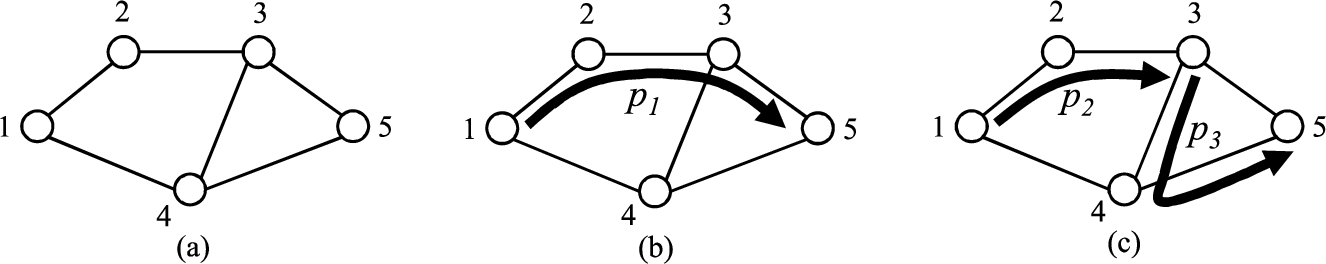
The process of finding a source-destination path consisting of a single lightpath is referred to as single-hop routing, where one hop corresponds to a lightpath which may consist of one or more physical hops in the network. For example, Fig. 1(b) shows a path
Fig. 1.
(a) A network with 5 nodes. (b) Single-hop routing. (c) Multi-hop routing.
This paper develops an auxiliary graph for the purpose of routing and path selection and proposes a dynamic multi-hop multipath RMSA and traffic grooming algorithm. In contract to the auxiliary graph proposed in [13], the weights on the edges in the auxiliary graph developed in this paper are based on a novel weight that incorporate spectrum fragmentation status, spectrum misalignment status, and spectrum usage. The contributions of this paper are as follows. First of all, this paper proposes a novel lightpath weight that is a combination of the number of spectrum slots, spectrum fragmentation, and spectrum misalignment to assess the potential effect of a lightpath on the availability of network resource. Second, this paper develops an auxiliary graph based on the lightpath weight and proposes a multi-hop multipath RMSA and traffic grooming algorithm based on the auxiliary graph. Finally, via simulation, this paper shows that the proposed dynamic multi-hop multipath RMSA and traffic grooming yields lower bandwidth blocking ratio than best multipath algorithm proposed in [13].
The rest of this paper is organized as follows. The weight assigned to a lightpath will be explained in the next section. The proposed dynamic multi-hop multipath RMSA and traffic grooming algorithm will then be described in Section 3. The worst case computational complexity of the proposed algorithm will be presented in Section 4. The performance of the proposed dynamic multi-hop multipath RMSA and traffic grooming algorithm will be studied in Section 5. Finally, some concluding remarks will be given in Section 6.
2.Lightpath weight
A lightpath weight assigned to a lightpath is used to evaluate the potential effect of the spectrum slots occupied by the lightpath on provisioning upcoming connection requests. The lightpath weight is related to (i) the number of spectrum slots occupied by the lightpath, (ii) spectrum fragmentation, and (iii) spectrum misalignment induced by the lightpath. The lightpath weight will be used for assigning weights on the edges in an auxiliary graph in the proposed dynamic multi-hop multipath RMSA and traffic grooming algorithm.
2.1.Number of spectrum slots
The number of spectrum slots for establishing a lightpath for provisioning a connection request includes the number of spectrum slots for data transmission, the number of reserved spectrum slots (if any), and the number of guard band slots (if any), where the reserved slots are reserved using the spectrum reservation scheme employed in [13]. The number of data slots is calculated based on the bandwidth requirement of the connection request, the selected modulation format, and the symbol rate per subcarrier. The number of guard band slots for the lightpath depends on whether the optical grooming mechanism is used. If the optical grooming mechanism is not used, guard band slots are required around the data slot(s). On the other hand, when the optical grooming mechanism is employed, no guard band is needed to separate the lightpath from the side-by-side lightpath along the common portion of the routes of the two lightpaths [16,35]. Let
Fig. 2.
A lightpath p in a network with 5 nodes.
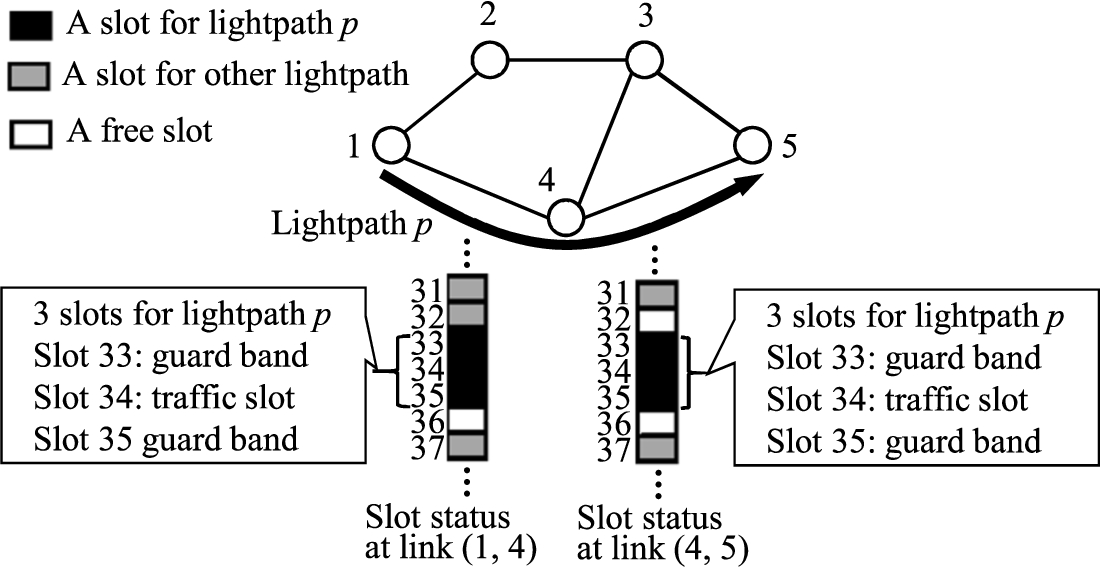
For example, lightpath p in Fig. 2 originated at node 1 and terminated at node 5 along route
The total number of spectrum slots required to establish a lightpath p is normalized to a value between 0 and 1 by dividing it by its largest possible value. The widest lightpath can occupy all spectrum slots supported by a sliceable transponder. Let
Suppose that two shortest paths between any pair of nodes in the example network in Fig. 2 are used for establishing lightpaths, i.e., the value of K is 2. For the example network shown in Fig. 2, the route with the largest number of physical hops among the K (
2.2.Spectrum fragmentation
Spectrum fragments of various sizes in terms of spectrum slots are created as lightpaths are established and torn down dynamically. Compared with a spectrum fragment of small size, a spectrum fragment of large size is more flexible for provisioning upcoming connection requests with different bandwidth requirements. A spectrum fragment of large size also has larger number of alternatives for accommodating a connection request with a given bandwidth requirement. It is preferable to use a smaller spectrum fragment to establish a lightpath to provision a connection request leaving spectrum fragments of larger sizes for upcoming connection requests.
This paper defines the fragmentation cost of a lightpath as the sum of the sizes of the spectrum fragments created by the lightpath. Let
The fragmentation cost of lightpath p is normalized to a value between 0 and 1 by dividing it by its largest possible value. The largest possible value of the fragmentation cost of a lightpath p is less than the number of spectrum slots on an optical fiber multiplied by H. Let the number of spectrum slots on an optical fiber be denoted by
For the example network and lightpath p in Fig. 2, the number of contiguous free spectrum slots with immediate lower indices than the spectrum slots used by lightpath p at link
2.3.Spectrum misalignment
The concept of spectrum “misalignment” has been described in [31,32] as one that breaks the continuity of available spectrum slots between a link and a neighbor link when a lightpath is established. The definition of the number of spectrum misalignments in [32] counts the number of breaks of spectrum continuity created due to the establishment of the lightpath. While the definition in [31] adds the number of spectrum misalignments created and deducts the number of spectrum misalignments vanished due to the establishment of the lightpath. We are concerned with the effect of the spectrum misalignments created by a lightpath on the provision of upcoming connection requests. Thus, this paper adopts the definition in [32].
Let
Fig. 3.
(a) A lightpath p in a network with 5 nodes. (b) Misalignments created due to the allocation of slots 33, 34, and 35 to lightpath p at link
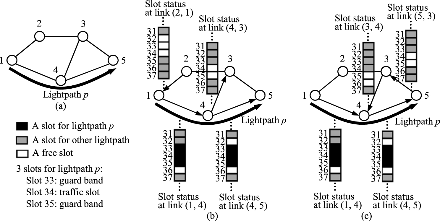
For example, Fig. 3(b) shows that, when spectrum slots 33, 34, and 35 are allocated to lightpath p at link
The total number of misalignments created by lightpath p is normalized to a value between 0 and 1 by dividing it by the maximum number of misalignments that can be created by a lightpath. To find the maximum possible number of misalignments, we assume that the degree of all of the nodes in the network are D, where D is the largest degree of the nodes in the network. The maximum number of spectrum slots that can be used to establish a light path is the maximum number of spectrum slots supported by a transponder
The largest degree of the nodes in the network in Fig. 3 is 3, i.e.,
The larger the number of spectrum misalignments in the network, it is more difficult for an RSA/RMSA algorithm to find a routing path that satisfies the spectrum continuity constraint. Thus, it is preferable to use a lightpath that yields smaller number of spectrum misalignments to provision a connection request. Hopefully, the RSA/RMSA algorithm has higher probability to successfully find lightpaths(s) to provision upcoming connection requests.
In recent years, the channel slicing and stitching technology [6] has been proposed to remove the spectrum continuity constraint such that misaligned spectrum slots can be allocated to a lightpath. If this technology is adopted in an EON network in which all nodes are equipped with sufficient number of splitting components and stitching components such that splitting process and stitching process can be performed whenever required even at intermediate nodes along any routing path, the spectrum continuity constraint can be completely removed and the spectrum-misalignment term in the lightpath weight can be dropped. However, if the splitting process or stitching process cannot be carried out at any of the nodes when required (i.e., the spectrum continuity constraint must be observed at the node for certain pair of links), the spectrum-misalignment term can be used to reflect this effect to some extent. Example situation where splitting process may not be able to be performed is that each node in the network is equipped with a limited number of slicers [2,18] or that only a subset of the nodes in the network are equipped with slicers [2]. In the EON networks considered in this paper, the channel slicing and stitching technology is not adopted.
2.4.Lightpath weight of a lightpath p
Calculation of the lightpath weight of a lightpath p depends on whether p is an existing lightpath or a candidate lightpath to be established. Let
For an existing lightpath p, grooming traffic onto p electrically does not create additional spectrum fragmentation or misalignment or occupy extra spectrum slots. Among different existing lightpaths that can be used to provision the traffic, it is desirable to use an existing light path that occupies smaller number of spectrum slots. Therefore, the normalized number of spectrum slots of existing lightpath p is used as its lightpath weight, i.e.,
3.Dynamic multi-hop multipath RMSA and traffic grooming algorithm
In the proposed algorithm, each path used to provision a connection request may consist of a single lightpath or multiple concatenated lightpaths. The proposed algorithm first tries to use a single path with sufficient bandwidth to provision a connection request. If the connection request cannot be fulfilled using a single path, the proposed algorithm tries to find multiple paths to provision the connection request. The proposed dynamic multi-hop multipath RMSA and traffic grooming algorithm finds each path based on an auxiliary graph. In the following, the auxiliary graph will first be described. The multi-hop multipath RMSA and traffic grooming algorithm will then be given.
3.1.Auxiliary graph
An auxiliary graph is constructed based on the topology of the network, a target bandwidth to be satisfied, and the resource status of the network. The target bandwidth for constructing an auxiliary graph is either the remaining bandwidth of a connection request to be satisfied or the bandwidth of a maximum bandwidth path from the source node to the destination node of the connection request, whichever is smaller. The target bandwidth for constructing an auxiliary graph is denoted by
3.1.1.Single-lightpath edge
It is preferable to use an existing lightpath with sufficient residual bandwidth to provision a connection request. If there is at least one existing lightpath from node i to node j with residual bandwidth greater than or equal to the target bandwidth
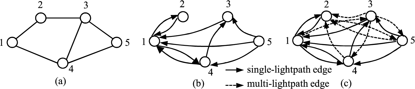
Figure 4(a) show a network with 5 nodes. Suppose that an existing lightpath with residual bandwidth greater than or equal to the target bandwidth
Fig. 4.
(a) A network with 5 nodes. (b) Auxiliary graph with only single-lightpath edges. (c) Auxiliary graph with single-lightpath and multi-lightpath edges.
3.1.2.Multi-lightpath edge
An attempt is made to add a multi-lightpath edge from vertex i to vertex j only when a single-lightpath edge has not been added. The flowchart for trying to add a multi-lightpath edge from vertex i to vertex j is presented in Fig. 5.
Fig. 5.
The flowchart for trying to add a multi-lightpath edge from vertex i to vertex j in the auxiliary graph.
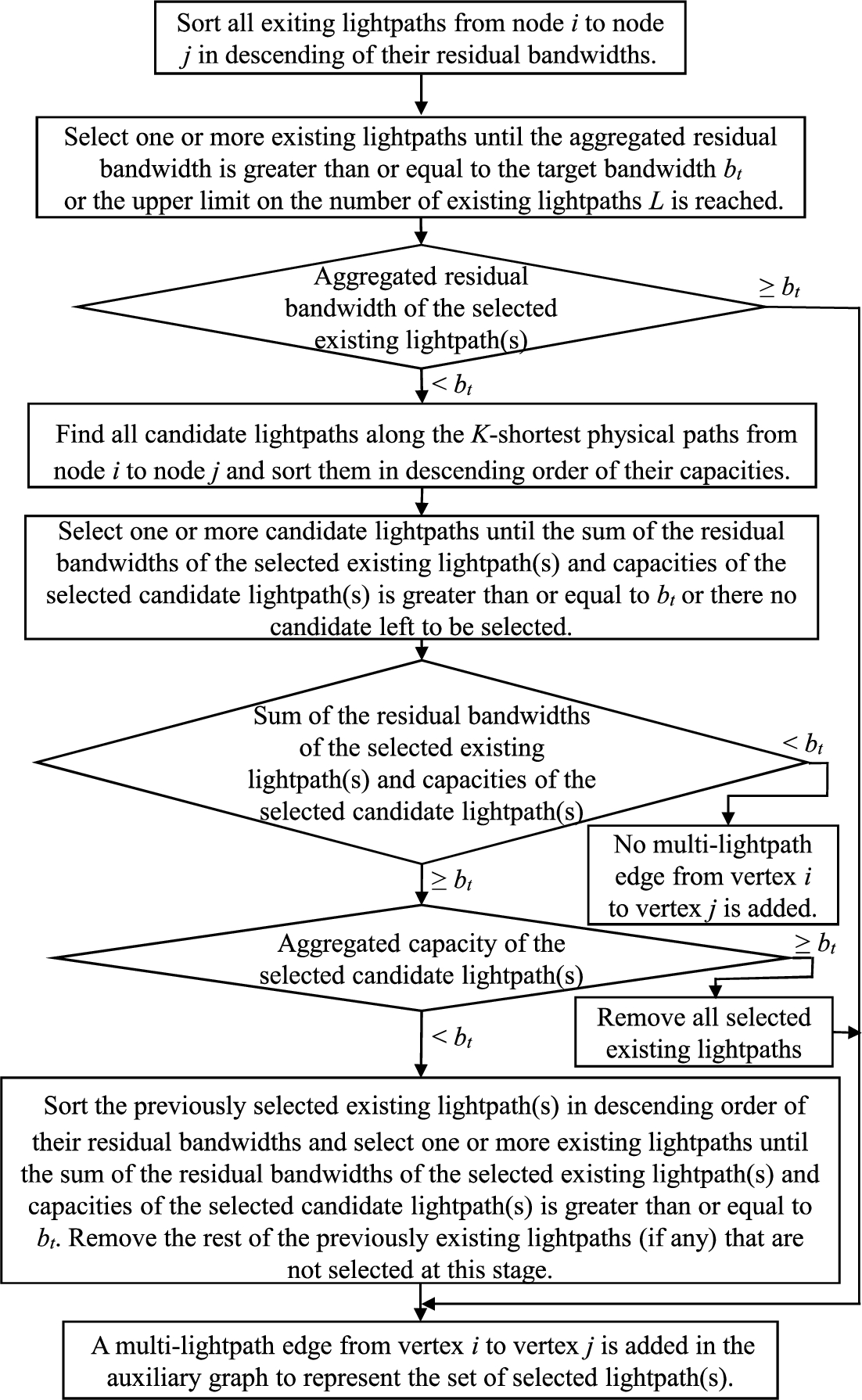
All exiting lightpaths from node i to node j are sorted according to their residual bandwidths with ties broken by giving priority to existing lightpaths with lower lightpath weights. Select one or more existing lightpaths until the aggregated residual bandwidth is greater than or equal to the target bandwidth
If the aggregated residual bandwidth of the selected existing lightpath(s) is less than
If the sum of the residual bandwidths of the selected existing lightpath(s) and capacities of the selected candidate lightpath(s) is greater than or equal to
In Fig. 4(b), no single-lightpath edge was added between each of the following node pairs:
3.1.3.Edge weights
The weight on an edge in the auxiliary graph is assigned based on the sum of the lightpath weight(s) of the set of lightpath(s) it represents. Using existing lightpath(s) to provision a connection request is preferable than establishing new lightpath(s). Thus, a large constant is added to the weight of an edge for each candidate lightpath in the set of lightpath(s) it represents in addition to the total lightpath weights of the lightpath(s) in the set. The value of the constant is selected such that the sum of the constant and the lightpath weight of a candidate lightpath is larger than sum of the lightpath weights of the largest possible number of existing lightpaths.
3.2.The algorithm
When a connection request
Two types of auxiliary graphs are used in the algorithm for finding one or more sd-paths to provision the connection request. The first type of auxiliary graphs consists of only single-lightpath edges among the node pairs. The second type of auxiliary graphs contains both single-lightpath and multi-lightpath edges among the node pairs. Let Ω denote the type of auxiliary graphs. The value of Ω is either S representing the first type or B denoting the second type. Let
Algorithm 1
Multi-hop algorithm
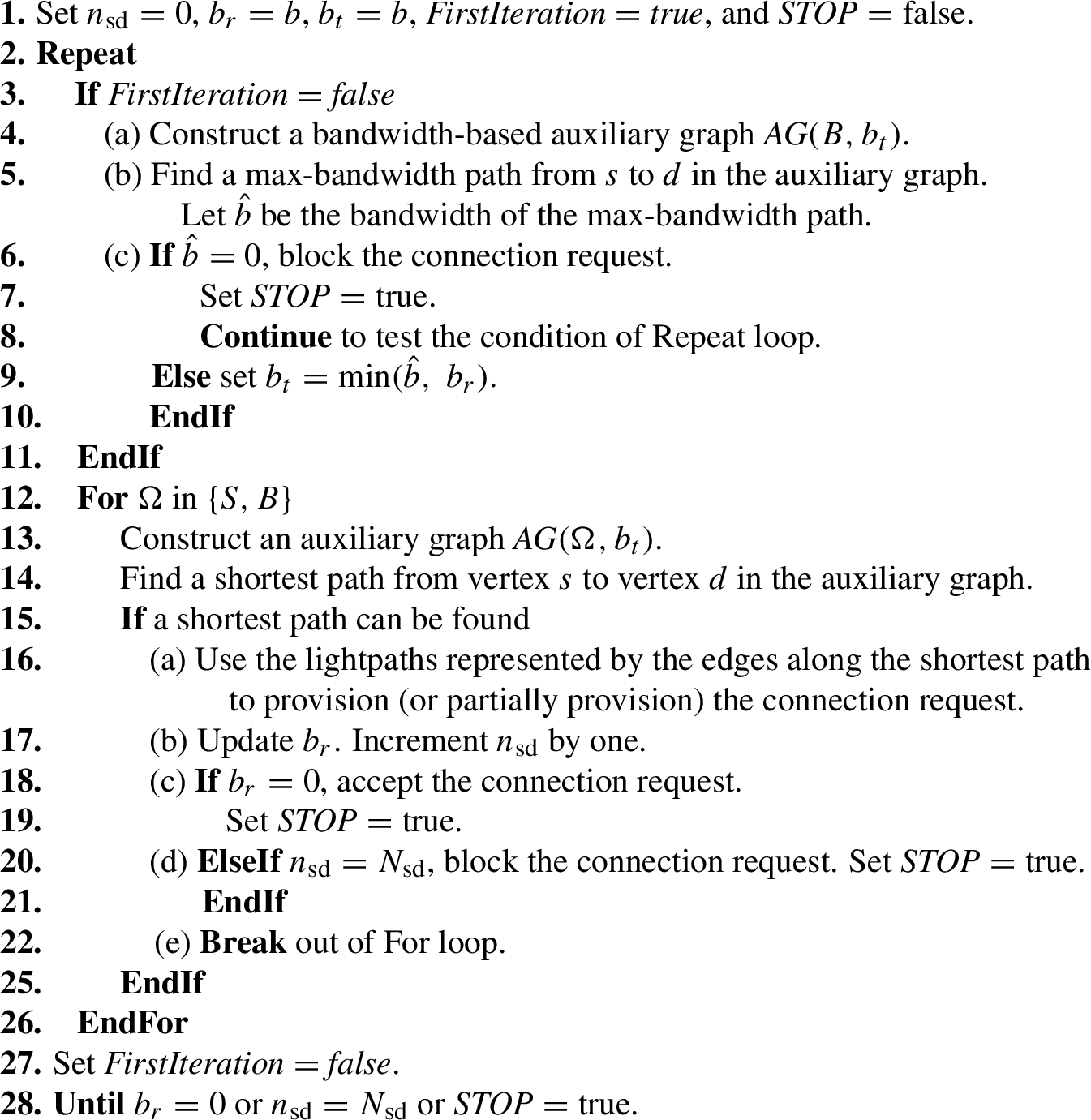
The proposed dynamic multi-hop multipath RMSA and traffic grooming algorithm is given in Algorithm 1. The proposed algorithm consists of a single-path phase and a multi-path phase. The term “single-path phase” is referring to the process of finding a single sd-path in the auxiliary graph. Similarly, the term “multi-path phase” is referring to the process of finding multiple sd-paths in the auxiliary graphs. The two phases are combined into a single iterative procedure (the Repeat-Until loop, lines 2 through 28). The first iteration of the algorithm is the single-path phase and the rest iterations belong to the multi-path phase. The multi-path phase is performed only when the single-path phase is unable to find a sd-path to provision the connection request.
Each iteration of the multi-hop algorithm consists of two parts. The first part of each iteration corresponds to the first loop of the For loop (lines 12 through 26) in which
The target bandwidth
At the beginning of each iteration except the first iteration, the algorithm finds the bandwidth of a maximum bandwidth path from the source node s to the destination node s by constructing a slightly different auxiliary graph and solves a max-bandwidth path problem [19] (lines 4 and 5). The auxiliary graph consists of both single-lightpath and multi-lightpath edges among the node pairs based on a target bandwidth of
Let
Then the first part of each iteration (the first loop of the For loop) tries to find a sd-path from source node s to destination node d in an auxiliary graph consisting of only single-lightpath edges among the node pairs (lines 13 and 14). If no sd-path can be found, the algorithm continues with the second part of the current iteration (the second loop of the For loop). On the other hand, if a sd-path can be found in the first part (line 15), the algorithm (i) uses the lightpaths represented by the edges along the sd-path to provision (or partially provision) the connection request (line 16), (ii) increments the number of sd-paths by one (line 17), (iii) updates the remaining bandwidth to be satisfied (line 17). If the remaining bandwidth to be satisfied is zero, accept the connection request and terminate the algorithm (lines 18 through 19). If the number of sd-paths reaches the upper limit
Figure 4 can be used as an example to briefly explain the proposed multi-hop multipath RMSA and traffic grooming algorithm. Let node 1 be the source node and node 5 be the destination node of an incoming connection request with a bandwidth requirement of b. Suppose that the first iteration of the Repeat-Until loop is not able to find any sd-path with sufficient bandwidth to provision the connection request, i.e., both the first and second loop of the For loop are unable to find a sd-path. The algorithm enters the second iteration of the Repeat-Until loop. The algorithm finds the bandwidth,
4.Computational complexity
The two most time consuming operations in the dynamic multi-hop multipath algorithm are constructing auxiliary graphs and finding sd-paths in auxiliary graphs. In the worst case, there are two directed edges connecting each pair of vertices in an auxiliary graph, one in each direction. Each edge represents one or more existing lightpaths or candidate lightpaths or both. In the worst case, the algorithm needs to find all candidate lightpaths between a pair of nodes and calculate their lightpath weights.
The weight of each candidate lightpath can be calculated in the process of finding the candidate lightpath. The worst case complexity for calculating the lightpath weight of a candidate lightpath is dominated by that of the computation of the spectrum misalignment term which involves checking the continuity status between the spectrum slots of a lightpath on a link and the same spectrum slots on neighboring links. To find all candidate lightpaths and their lightpath weights along the K shortest physical paths between s and d, the algorithm needs to go through all K shortest paths, all physical hops of each path, all spectrum slots at each link and its neighboring links. Hence, the worst case complexity for finding all candidate lightpaths along the K shortest physical paths between a pair of nodes and calculating their lightpath weights is of
As described previously, the worst case computational complexity for finding all candidate lightpaths between a pair of nodes and calculating their lightpath weights is of
The worst case computational complexity for finding a shortest sd-path in an auxiliary graph using the best shortest path algorithm is of
It is obvious that constructing auxiliary graphs has higher computational complexity than finding sd-paths in auxiliary graphs. Thus, the worst case computational complexity of the multi-hop multipath is dominated by that for constructing auxiliary graphs which is of
5.Performance study
The performance of the proposed dynamic multi-hop multipath RMSA and traffic grooming algorithm is studied via simulation. The performance of the proposed dynamic multi-hop multipath RMSA and traffic grooming algorithm is compared with that of an algorithm proposed in [13] since this is the only work that employs multi-hop routing among the previous works [5,9–11,13,14,17,33,34,37–39] on dynamic multipath RSA in EON. Among the three dynamic multi-hop multipath RMSA and traffic grooming algorithms proposed in [13], the MP-MSU algorithm yields the lowest request blocking ratio. Therefore, the performance of the algorithm proposed in this paper is compared with that of the MP-MSU algorithm proposed in [13]. Three versions of the proposed algorithm with three different values, namely, 1, 3, and infinity, for the limit on the number of sd-paths in the auxiliary graphs,
Four performance measures, namely, bandwidth blocking ratio, spectrum utilization factor, sub-transponder utilization factor, and average number of existing lightpaths per request are used in the simulation study. Ninety-five percent confidence interval is calculated for each data point obtained in the simulation results. The bandwidth blocking ratio is calculated as the total requested bandwidth of blocked connection requests to the total requested bandwidth of all connection requests.
The spectrum utilization factor is calculated in the following way. Let P be the set of lightpaths established during the simulation time and
The sub-transponder utilization factor is computed in the following manner. Let the number of transponders (or SBVTs) in the network be denoted by Θ and the number of sub-transponder contained in each transponder be denoted by θ. Each sub-transponder contains a transmitting side component and a receiving side component [27]. A lightpath occupies a transmitting side component of a sub-transponder at its originating node and a receiving side component of a sub-transponder at its terminating node during its holding time. For the purpose of calculating sub-transponder utilization factor, a transmitting side component and a receiving side component occupied by a lightpath can be counted as one sub-transponder although they are located at different nodes. The sub-transponder utilization factor is calculated as the following ratio
The average number of existing lightpaths per request is calculated as follows. The number of existing lightpaths used to provision each accepted connection request is counted when each is accepted. The average number of existing lightpaths per request is computed as the ratio of the total number of existing lightpaths used to provision all accepted connection requests to the number of accepted connection requests.
5.1.Simulation model
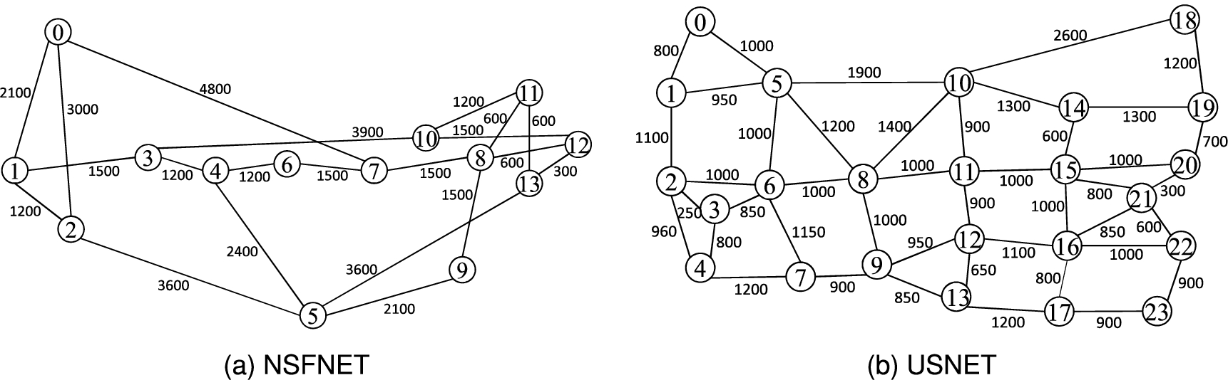
Two network topologies are used in our performance study, namely, the 14-node NSFNET with 21 bidirectional links and the 24-node USNET with 43 bidirectional links as shown in Figs 6(a) and 6(b) respectively. Each link consists of two optical fibers one in each direction. The lengths of the fibers in terms of kilometers are shown on the links in the figures. The total number of available spectrum slots on each fiber is 320 and the width of each spectrum slot is 12.5 GHz. For a lightpath without employing the optical grooming mechanism, guard bands are added on both sides of the traffic slot(s). The width of each guard band is one spectrum slot.
The number of SBVTs in each node is 48 multiplied by the degree of the node. Each SBVT consists of 3 sub-transponders. Each SBVT is able to support up to 10 sub-carriers and 4 modulation formats, namely, BPSK, QPSK, 8-QAM, and 16-QAM. For simplicity, it is assumed that SNR (signal to noise ratio) loss in the EON nodes can be compensated such that transmission reach for a given modulation format is a fixed distance. Techniques for compensation of SNR losses due to various components in the nodes have been discussed in [22]. With the above assumption, the transmission reach for QPSK is selected to be 7,200 Km [7]. The transmission reaches for BPSK, 8-QAM, and 16-QAM are chosen respectively to be 14,400 Km, 3,600 Km and 1,800 Km according to the half-distance law [4].
Connection requests are assumed to arrive at the network according to Poisson process with a mean arrival rate of λ per time unit. Holding times of connection requests are assumed to be exponentially distributed with a mean of one time unit. Bandwidth requirement of each connection request is randomly selected among 10 Gbps, 40 Gbps, 100 Gbps, and 160 Gbps.
The source and destination nodes of each connection request are selected in the following manner. For the NSFNET topology, measured traffic data [21] is used to derive the probabilities for selecting source and destination nodes. The probability that a node is selected as the source node of a connection request is calculated as the ratio of the amount of outgoing traffic of the node to the total amount of outgoing traffic of all nodes. Given a selected source node i, the probability that node j,
Fig. 6.
(a) The topology of the 14-node NSFNET with 21 bidirectional links. (b) The topology of the 24-node USNET with 43 bidirectional links.
For the USNET topology, a guideline for generating non-uniform traffic [26] is used to derive the probabilities for selecting source and destination nodes. The nodes are classified into “Large” nodes and “Small” nodes. Six of the nodes, namely, nodes 5, 6, 8, 10, 15, and 16, are selected as “Large” nodes and the rest of the nodes are “Small” nodes. Traffic distribution among the nodes is as follows: Large-Large: 40%, Large-Small: 40%, Small-Small: 20%. The probabilities for selecting source and destination nodes are calculated based on the traffic distribution.
5.2.Comparison of bandwidth blocking ratios
Fig. 7.
Comparison of bandwidth blocking ratio.
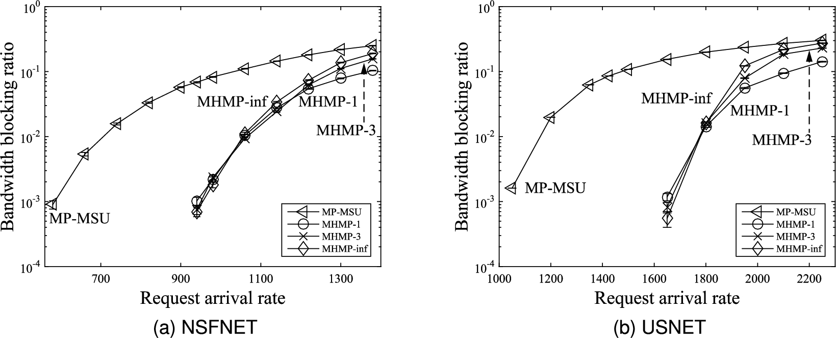
Figures 7(a) and 7(b) compare the bandwidth blocking ratios. It can be observed that all three versions of the proposed MHMP algorithm yield lower bandwidth blocking ratios than the MP-MSU algorithm proposed in [13]. The main reason is that the edge weight on each edge in the auxiliary graph used in the proposed MHMP algorithm is related to the lightpath weights of the set of the lightpaths represented by the edge, which in turn is related to the number of spectrum slots occupied by the lightpaths, spectrum fragmentation, and spectrum misalignment of the set of lightpaths represented by the edge. Whereas spectrum fragmentation and spectrum misalignment are not considered in the MP-MSU algorithm proposed in [13]. The proposed MHMP algorithm uses the minimum-weight sd-path in the auxiliary graph to provision a connection request implying that lightpaths with less number of spectrum slots, less spectrum fragmentation, and less spectrum misalignment are selected to provision the connection request. Thus, the lightpaths along the minimum-weight sd-path induce less spectrum fragmentation and less spectrum misalignment leading to more useful available spectrum resource for provisioning upcoming connection requests resulting in lower bandwidth blocking ratio.
Comparing the proposed MHMP algorithm with different values for the limit on the number of sd-paths in the auxiliary graphs, when the traffic load is low, in general, the higher the limit on the number sd-paths in the auxiliary graphs the lower the bandwidth blocking ratio. In other words, the MHMP-inf algorithm yields lower bandwidth blocking ratio than the MHMP-3 algorithm and the MHMP-3 algorithm yields lower bandwidth blocking ratio than the MHMP-1 algorithm. The reason is that spectrum resource in the network is abundant when the traffic load is low. With abundant spectrum resource, the proposed MHMP algorithm with higher limit on the number sd-paths is able to use more lightpaths to try to fulfill more connection requests resulting in lower bandwidth blocking ratio. However, when the traffic load is medium to high, spectrum resource in the network is somewhat rare to rare. The proposed MHMP algorithm with lower limit on the number sd-paths uses spectrum resource relatively more conservatively leaving more spectrum resource for upcoming connection requests. Thus, the proposed MHMP algorithm with lower limit on the number sd-paths is able to yield lower bandwidth blocking ratio.
5.3.Comparison of spectrum utilization factors
Fig. 8.
Comparison of spectrum utilization factors.
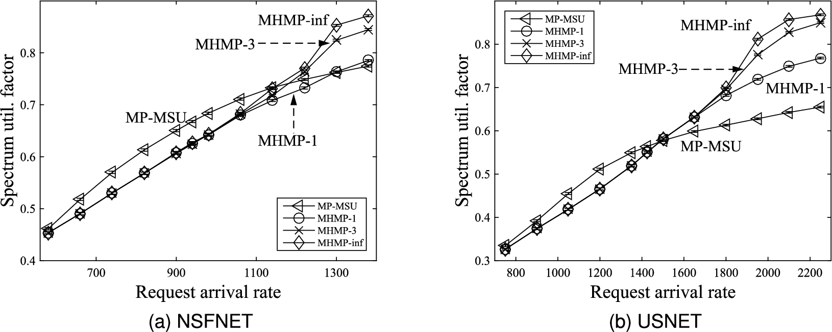
Figures 8(a) and 8(b) show the spectrum utilization factors. It can be observed that, when the traffic load is low, all three versions of the proposed MHMP algorithm yield lower spectrum utilization factors than the MP-MSU algorithm proposed in [13]. The reason is that the proposed MHMP algorithm prefers to utilize residual bandwidths of existing lightpaths to provision connection requests, whereas the MP-MSU algorithm does not give priority to using residual bandwidths of existing lightpaths. When the traffic load is low, it is likely that residual bandwidths of existing lightpaths can be found to provision connection requests without establishing new lightpaths resulting in lower spectrum utilization factors for the three versions of the proposed MHMP algorithm than the MP-MSU algorithm proposed in [13].
As the traffic load increases, residual bandwidths of existing lightpaths and available spectrum slots along sd-paths with smaller number of hops become scarce. Giving priority to using residual bandwidths of existing lightpaths may need to use residual bandwidths of existing lightpaths along sd-paths with larger number of hops requiring more bandwidth for provisioning connection requests. Thus, when the traffic load is high, all three versions of the proposed MHMP algorithm yield higher spectrum utilization factors than the MP-MSU algorithm proposed in [13]. This phenomenon is more evident as the limit on the number sd-paths increases for the proposed MHMP algorithm. The proposed MHMP algorithm with larger limit on the number sd-paths yields higher spectrum utilization factor.
5.4.Comparison of sub-transponder utilization factors
Fig. 9.
Comparison of sub-transponder utilization factors.
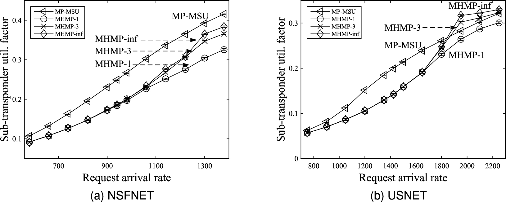
Figures 9(a) and 9(b) compare the sub-transponder utilization factors. It can be observed that all three versions of the proposed MHMP algorithm yield lower sub-transponder utilization factors than the MP-MSU algorithm proposed in [13] except when the traffic load is high in the USNET topology. The reason is that all three versions of the proposed MHMP algorithm prefer to use residual bandwidths of existing lightpaths to provision connection requests; i.e., sharing sub-transponders of existing lightpaths is preferable than using free sub-transponders to establish new lightpaths. The MP-MSU algorithm proposed in [13] also employs electrical grooming mechanism; however, no preference is given to using residual bandwidths of existing lightpaths. Hence, all three versions of the proposed MHMP algorithm use electrical grooming mechanism significantly more frequently than the MP-MSU algorithm. Therefore, all three versions of the proposed MHMP algorithm yield lower sub-transponder utilization factors than the MP-MSU algorithm.
When the traffic load is high in the USNET topology, the proposed MHMP algorithm having a limit on the number of sd-path of three or infinity yields higher sub-transponder utilization factor than the MP-MSU algorithm. This is because the USNET topology has larger number of nodes and links compared with the NSFNET topology. Hence, there are more alternatives for finding an sd-path between each pair of nodes in the USNET topology. When the traffic load is high, the residual bandwidths of existing lightpaths and available spectrum slots are scarce along sd-paths with smaller number of hops and smaller number of concatenated lightpaths. The MHMP-3 and MHMP-inf algorithms allow more sd-paths to be used to provision each connection request than the MHMP-1 and MP-MSU algorithms. Therefore, in the USNET topology, it is more likely that the MHMP-3 and MHMP-inf algorithms use sd-paths with larger number of concatenated existing lightpaths or new lightpaths at high traffic load to provision connection requests resulting in occupying larger number of sub-transponders.
5.5.Comparison of average number of existing lightpaths per request
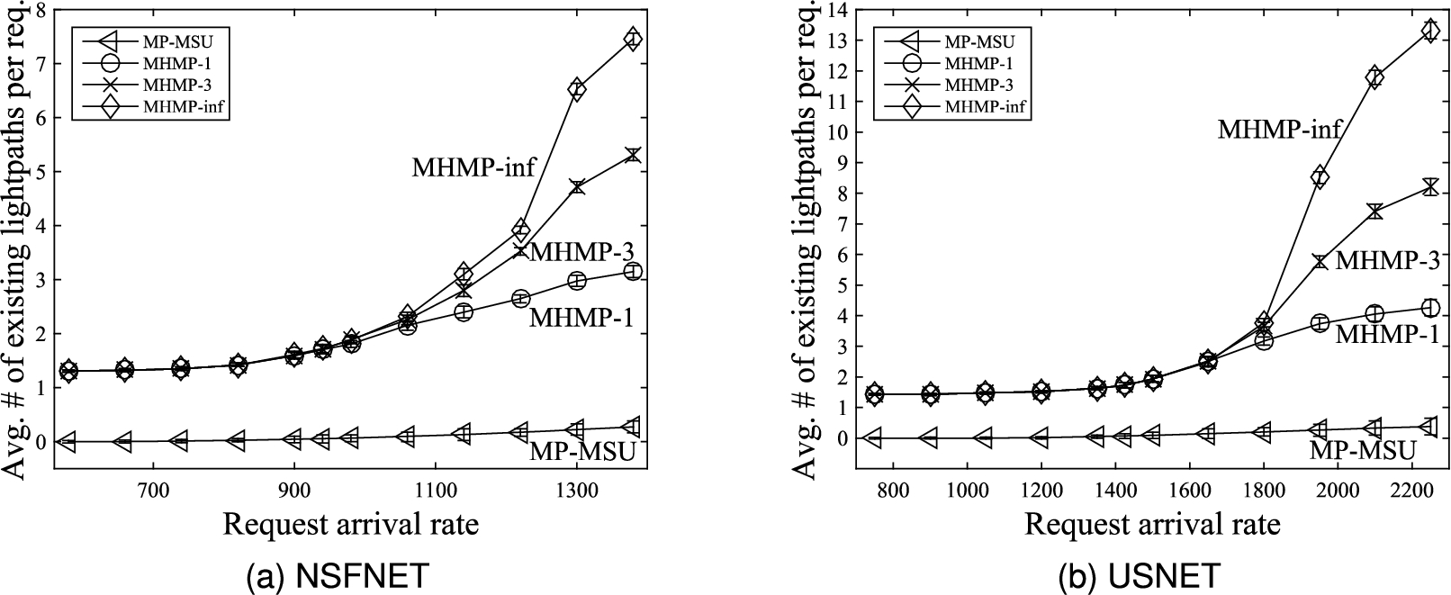
Figures 10(a) and 10(b) show the average number of existing lightpaths per request. It can be observed that all three versions of the proposed MHMP algorithm yield higher average number of existing lightpaths per request than the MP-MSU algorithm proposed in [13]. This is because all three versions of the proposed MHMP algorithm prefer to use electrical grooming mechanism to groom traffic of connection requests onto existing lightpaths with residual bandwidths. In contrast, the MP-MSU algorithm proposed in [13] does not give priority to using electrical grooming mechanism although it also employs electrical grooming mechanism.
The two figures also show that the average number of existing lightpaths per request increases as the traffic load increases. As the traffic load increases, on the average, the residual bandwidth of each existing lightpath decreases since the average bandwidth of the traffic carried by each existing lightpath increases when the traffic load increases. With smaller average residual bandwidth in each existing lightpath, it is likely that a larger number of existing lightpaths is used to fulfill a connection request.
Comparing the three versions of the proposed MHMP algorithm, the average number of existing lightpaths per request increases as the limit on the number of sd-paths increases, i.e., the MHMP-inf algorithm yields higher average number of existing lightpaths per request than the MHMP-3 algorithm and the MHMP-3 algorithm yields higher average number of existing lightpaths per request than the MHMP-1 algorithm. The average number of sd-paths used to provision a connection request increases as the limit on the number of sd-paths increases. A larger number of sd-paths is likely to contain a greater number of existing lightpaths. Thus, the average number of existing lightpaths per request increases as the limit on the number of sd-paths increases.
Fig. 10.
Comparison of average number of existing lightpaths per request.
6.Conclusion
The dynamic multi-hop multipath RMSA and traffic grooming problem in OFDM-based sliceable elastic optical networks has been studied in this paper. A lightpath weight that combines the number of spectrum slots, spectrum fragmentation, and spectrum misalignment has been used to evaluate the potential effect of a lightpath on the availability of network resource. An auxiliary graph has been developed to aid finding source-destination path(s) for provisioning connection requests. Based on the auxiliary graph, this paper has proposed a dynamic multi-hop multipath RMSA and traffic grooming algorithm. Simulation has been carried out to show that the proposed algorithm is able to yield low bandwidth blocking ratio.
Acknowledgements
This research was supported by the Ministry of Science and Technology, Taiwan, under grant MOST 109-2221-E-007-078.
Conflict of interest
None to report.
References
[1] | F.S. Abkenar and A.G. Rahbar, Study and analysis of routing and spectrum allocation (RSA) and routing, modulation and spectrum allocation (RMSA) algorithms in elastic optical networks (EONs), Opt. Switch. Netw. 23: ((2017) ), 5–39. doi: 10.1016/j.osn.2016.08.003. |
[2] | K. Akaki, P. Pavarangkoon and N. Kitsuwan, Elastic optical network for fragmented bandwidth allocation with limited slicers, in: Proceedings of the 13th IEEE International Conference on Information Technology and Electrical Engineering (ICITEE), (2021) , pp. 1–4. |
[3] | R. Alvizu, V. Soto, S. Troia and G. Maier, Enabling multipath optical routing with hybrid differential delay compensation, in: 20th IEEE International Conference on Transparent Optical Networks (ICTON), (2018) , pp. 1–4. |
[4] | A. Bocoi, M. Schuster, F. Rambach, M. Kiese, C.A. Bunge and B. Spinnler, Reach-dependent capacity in optical networks enabled by OFDM, in: Proc. Optical Networking and Commun. Conf. (OFC), (2009) . |
[5] | A. Cai, L. Peng and G. Shen, Sub-band virtual concatenation lightpath blocking performance evaluation for CO-OFDM optical networks, in: Proceedings of the OSA Asia Communications and Photonics Conference, 2012, November, (2012) , pp. AS4D-3. doi: 10.1364/ACPC.2012.PAF4D.3. |
[6] | Y. Cao, A. Almaiman, M. Ziyadi, A. Mohajerin-Ariaei, C. Bao, P. Liao, F. Alishahi et al., Reconfigurable channel slicing and stitching for an optical signal to enable fragmented bandwidth allocation using nonlinear wave mixing and an optical frequency comb, Journal of Lightwave Technology 36: (2) ((2018) ), 440–446. doi: 10.1109/JLT.2017.2750168. |
[7] | S. Chandrasekhar, X. Liu, B. Zhu and D.W. Peckham, Transmission of a 1.2-Tb/s 24-carrier no-guard-interval coherent OFDM superchannel over 7200-km of ultra-large-area fiber, in: Proc. ECOC, (2009) . |
[8] | B.C. Chatterjee, N. Sarma and E. Oki, Routing and spectrum allocation in elastic optical networks: A tutorial, IEEE Commun. Surveys & Tutorials 17: (3) ((2015) ), 1776–1800. doi: 10.1109/COMST.2015.2431731. |
[9] | X. Chen, Y. Zhong and A. Jukan, Multipath routing in elastic optical networks with distance-adaptive modulation formats, in: Proceedings of the IEEE International Conference on Communications (ICC), (2013) , pp. 3915–3920. |
[10] | S. Dahlfort, M. Xia, R. Proietti and S.J.B. Yoo, Split spectrum approach to elastic optical networking, in: Proceedings of the OSA European Conference and Exhibition on Optical Communication, (2012) , pp. Tu-3. |
[11] | Z. Fan, Y. Qiu and C.K. Chan, Dynamic multipath routing with traffic grooming in OFDM-based elastic optical path networks, Journal of Lightwave Technology 33: (1) ((2015) ), 275–281. doi: 10.1109/JLT.2014.2387312. |
[12] | O. Gerstel, M. Jinno, A. Lord and S.B. Yoo, Elastic optical networking: A new dawn for the optical layer?, IEEE Commun. Mag. 50: (2) ((2012) ), S12–S20. doi: 10.1109/MCOM.2012.6146481. |
[13] | S.M.H. Ghazvini, A.G. Rahbar and B. Alizadeh, Load balancing, multipath routing and adaptive modulation with traffic grooming in elastic optical networks, Computer Networks 169: ((2020) ), 107081. doi: 10.1016/j.comnet.2019.107081. |
[14] | T. Hashimoto, K.I. Baba and S. Shimojo, Optical path splitting methods for elastic optical network design, in: Proceedings of the OSA Asia Communications and Photonics Conference, (2015) , pp. AS4H-4. |
[15] | M. Jinno, H. Takara, B. Kozicki, Y. Tsukishima, Y. Sone and S. Matsuoka, Spectrum-efficient and scalable elastic optical path network: Architecture, benefits, and enabling technologies, IEEE Commun. Mag. 47: (11) ((2009) ), 66–73. doi: 10.1109/MCOM.2009.5307468. |
[16] | M. Jinno, H. Takara, Y. Sone, K. Yonenaga and A. Hirano, Multi-flow optical transponder for efficient multilayer optical networking, IEEE Commun. Mag. 50: (5) ((2012) ), 56–65. doi: 10.1109/MCOM.2012.6194383. |
[17] | N. Kadu, S. Shakya and X. Cao, Modulation-aware multipath routing and spectrum allocation in elastic optical networks, in: Proceedings of the IEEE International Conference on Advanced Networks and Telecommunications Systems (ANTS), (2014) , pp. 1–6. |
[18] | N. Kitsuwan, K. Akaki, P. Pavarangkoon and A. Nag, Spectrum allocation scheme considering spectrum slicing in elastic optical networks, Journal of Optical Communications and Networking 13: (7) ((2021) ), 169–181. doi: 10.1364/JOCN.422915. |
[19] | N. Malpani and J. Chen, A note on practical construction of maximum bandwidth paths, Information Processing Letters 83: (3) ((2002) ), 175–180. doi: 10.1016/S0020-0190(01)00323-4. |
[20] | S. Miladić-Tešić, G. Marković and V. Radojičić, Traffic grooming technique for elastic optical networks: A survey, Optik 176: ((2019) ), 464–475. doi: 10.1016/j.ijleo.2018.09.068. |
[21] | B. Mukherjee, D. Banerjee and S. Ramamurthy, Some principles for designing a wide-area WDM optical network, IEEE/ACM Trans. Netw. 4: (5) ((1996) ), 684–696. doi: 10.1109/90.541317. |
[22] | A. Napoli, D. Rafique, M. Bohn, M. Nölle, J.K. Fischer and C. Schubert, Transmission in elastic optical networks, in: Elastic Optical Networks, Springer, Cham, (2016) , pp. 83–116. |
[23] | A. Pagès, J. Perelló, S. Spadaro and J. Comellas, Optimal route, spectrum, and modulation level assignment in split-spectrum-enabled dynamic elastic optical networks, Journal of Optical Communications and Networking 6: (2) ((2014) ), 114–126. doi: 10.1364/JOCN.6.000114. |
[24] | A. Pagès, J. Perelló, S. Spadaro and G. Junyent, Split spectrum-enabled route and spectrum assignment in elastic optical networks, Optical Switching and Networking 13: ((2014) ), 148–157. doi: 10.1016/j.osn.2014.04.002. |
[25] | L. Ruiz, R.J.D. Barroso, I. De Miguel, N. Merayo, J.C. Aguado and E.J. Abril, Routing, modulation and spectrum assignment algorithm using multi-path routing and best-fit, IEEE Access 9: ((2021) ), 111633–111650. doi: 10.1109/ACCESS.2021.3101998. |
[26] | A.A.M. Saleh, Dynamic multi-terabit core optical networks: Architecture, protocols, control and management (CORONET), in: DARPA BAA, (2006) , pp. 06-29. |
[27] | N. Sambo, P. Castoldi, A. D’Errico, E. Riccardi, A. Pagano, M.S. Moreolo, J.M. Fabrega et al., Next generation sliceable bandwidth variable transponders, IEEE Communications Magazine 53: (2) ((2015) ), 163–171. doi: 10.1109/MCOM.2015.7045405. |
[28] | S. Talebi, F. Alam, I. Katib, M. Khamis, R. Salama and G.N. Rouskas, Spectrum management techniques for elastic optical networks: A survey, Optical Switching and Networking 13: ((2014) ), 34–48. doi: 10.1016/j.osn.2014.02.003. |
[29] | U. Ujjwal, N. Mahala and J. Thangaraj, Dynamic adaptive spectrum allocation in flexible grid optical network with multi-path routing, IET Communications 15: ((2021) ), 211–223. doi: 10.1049/cmu2.12046. |
[30] | X. Wang, G. Shen, Z. Zhu and X. Fu, Benefits of sub-band virtual concatenation for enhancing availability of elastic optical networks, Journal of Lightwave Technology 34: (4) ((2016) ), 1098–1110. doi: 10.1109/JLT.2015.2509605. |
[31] | Y. Yin, H. Zhang, M. Zhang, M. Xia, Z. Zhu, S. Dahlfort and S.B. Yoo, Spectral and spatial 2D fragmentation-aware routing and spectrum assignment algorithms in elastic optical networks, IEEE/OSA Journal of Optical Communications and Networking 5: (10) ((2013) ), A100–A106. doi: 10.1364/JOCN.5.00A100. |
[32] | Y. Yin, M. Zhang, Z. Zhu and S.J.B. Yoo, Fragmentation-aware routing, modulation and spectrum assignment algorithms in elastic optical networks, in: Proceedings of the OSA Optical Fiber Communication Conference, (2013) , pp. OW3A-5. |
[33] | F. Yousefi and A.G. Rahbar, Novel fragmentation-aware algorithms for multipath routing and spectrum assignment in elastic optical networks-space division multiplexing (EON-SDM), Optical Fiber Technology 46: ((2018) ), 287–296. doi: 10.1016/j.yofte.2018.11.002. |
[34] | F. Yousefi, A.G. Rahbar and M. Yaghubi-Namaad, Fragmentation-aware algorithms for multipath routing and spectrum assignment in elastic optical networks, Optical Fiber Technology 53: ((2019) ), 102019. doi: 10.1016/j.yofte.2019.102019. |
[35] | G. Zhang, M. De Leenheer and B. Mukherjee, Optical traffic grooming in OFDM-based elastic optical networks [invited], Journal of Optical Commun. and Networking 4: (11) ((2012) ), B17–B25. doi: 10.1364/JOCN.4.000B17. |
[36] | Y. Zhang, L. Li, Y. Li, S.K. Bose and G. Shen, Spectrally efficient operation of mixed fixed/flexible-grid optical networks with sub-band virtual concatenation, in: Proceedings of the IEEE 18th International Conference on Transparent Optical Networks (ICTON), (2016) , pp. 1–4. |
[37] | R. Zhu, J.P. Jue, A. Yousefpour, Y. Zhao, H. Yang, J. Zhang, X. Yu and N. Wang, Multi-path fragmentation-aware advance reservation provisioning in elastic optical networks, in: Proceedings of the IEEE Global Communications Conference (GLOBECOM), (2016) , pp. 1–6. |
[38] | R. Zhu, Y. Zhao, H. Yang, X. Yu, J. Zhang, A. Yousefpour, N. Wang and J.P. Jue, Dynamic time and spectrum fragmentation-aware service provisioning in elastic optical networks with multi-path routing, Optical Fiber Technology 32: ((2016) ), 13–22. doi: 10.1016/j.yofte.2016.08.009. |
[39] | Z. Zhu, W. Lu, L. Zhang and N. Ansari, Dynamic service provisioning in elastic optical networks with hybrid single-/multi-path routing, Journal of Lightwave Technology 31: (1) ((2013) ), 15–22. doi: 10.1109/JLT.2012.2227683. |


