
Migration of different LNAPLs in subsurface under groundwater fluctuating conditions by the simplified image analysis method
Abstract
The correct understanding of the dynamic behavior of Light Non-Aqueous Phase Liquids (LNAPLs) under fluctuating groundwater conditions, difficult to test with conventional methods, is important for the adequate remediation of contaminated soils. In this study, we verified the suitability of the Simplified Image Analysis Method (SIAM) as a tool to assess the saturation distribution of water and Non-Aqueous Phase Liquids (NAPLs) in granular soils, by testing its basic assumption, the existence of a linear relationship between water saturation (Sw), NAPL saturation (So) and optical density (Di), for nine different NAPLs. We then utilized SIAM to study the dynamic behavior of four different LNAPLs that were infiltrated to 1D columns filled with Toyoura sand, and later subjected to two cycles of drainage-imbibition of the water table. It was found that, under similar conditions, the depth of LNAPL infiltration was linearly correlated to the viscosity of the contaminants (R2 = 0.84), the difference between the depth of the mobile fraction after both drainage and imbibition stages was linearly correlated to the interfacial tension values (R2 = 0.79), and the viscosity was logarithmically correlated to the residual saturation ratios for all different NAPLs (R2 = 0.95), correlations that can help us understand and predict the behavior of different contaminants when spilled in the ground.
1Introduction
Diesel, gasoline, motor oil, and most hydrocarbons are classified as Non Aqueous Phase Liquids (NAPLs), and are among the most important liquid contaminants of groundwater, a major source of water for human consumption [1–4]. A NAPL is a fluid that is immiscible in water and, as such, has a different behavior when released into the subsurface depending on its density relative to that of water: if it is a Light NAPL (LNAPL), it will migrate downward until it reaches the water table where it will float depressing the groundwater, whereas if it is a Dense NAPL (DNAPL) it will continue migrating until it reaches an impermeable layer. Natural phenomena such as rain, draughts, tides, variations in river discharge, etc., cause groundwater table fluctuations that particularly affect the migration of the LNAPLs that are already in the vadose zone [5–8]. While these natural phenomena are fairly common, most studies of LNAPLs as contaminants analyze their behavior under static or unidirectional dynamic conditions, due to the difficulty of studying multiple-cycle dynamic conditions [8–10].
In order to remediate LNAPL contaminated sites in an efficient and cost-effective manner, a correct understanding of the behavior of these contaminants under multiple groundwater fluctuation conditions is, therefore, essential. To accomplish this, accurate numerical models should be developed, calibrated, and validated using results from adequate quantitative laboratory experiments. These experiments should provide with the correct constitutive relations between pressure, saturation, and relative permeability (k-S-p) that will be used to solve the governing flow equations of multiphase flow. The relatively simple equation relating relative permeability to saturation, developed by van Genuchten [11], focused researchers into obtaining the simpler saturation-pore pressure (S-p) relation to fully characterize multiphase flow [7, 9, 10, 12, 13]. Measurement of pore pressure proves to be simple, with some of these researchers relying on mechanical set-ups that manually increase suction values [14, 15], while the others make use of pressure transducers to measure the produced pore pressure [7, 9, 16].
For the measurement of saturation, in contrast, no prevalent technique exists, and those that are mostly used can be roughly divided into two categories: the simple intrusive/destructive methods—such as gravimetric sampling—and the very complex and usually expensive non-intrusive/non-destructive methods—such as gamma ray [17], high-speed X-ray attenuation [18], and electrical conductivity probe [7]. Unfortunately, the former do not allow the monitoring of saturation values under dynamic conditions, and the latter do not allow its monitoring in the entire domain at one time.
Since the behavior of LNAPs is affected by groundwater fluctuation, and since a better understanding of their transport mechanism can be reached by monitoring the entire domain during the whole experimental stage, the Simplified Image Analysis Method (SIAM) was recently introduced as a tool to measure water and light non-aqueous phase liquids (LNAPLs) saturation distributions in whole domains when evaluating the effects of groundwater fluctuations on LNAPL migration in porous media [19]. This method was tested for paraffin liquid but, in order to confirm that it can be applied for other NAPLs as well, we have tested the base theory, the Beer-Lambert Law of Transmittance that establishes the existence of a linear relationship between optical density and the concentrations of the studied substances, for different additional NAPLs covering a wide range of density and viscosity values (0.73 ≤ ρ ≤ 1.20 g/cm3; 1.4 ≤ ν ≤ 1000 mPa · s). The main goal of this first stage of our study was to confirm that the use of different NAPLs with different physic-chemical properties would not preclude the required linear relationships from happening.
Once the validity of the Simplified Image Analysis Method (SIAM) was confirmed for different NAPLs, we have used this method to understand the importance of density, viscosity, and interfacial tension of four different LNAPLs, on their migrating behavior under fluctuating groundwater conditions, conditions that cannot be easily studied by either the intrusive/destructive methods or the non-intrusive/non-destructive methods described earlier.
2Theoretical background
2.1Image analysis
When a beam of parallel monochromatic radiation with power I0 strikes a block of absorbing matter perpendicular to a surface, after passing through a length b of the material (Fig. 1), the Beer-Lambert Law of Transmittance states that its power is decreased to It as a result of absorption:
(1)
where I0 is the initial radiant power, It the transmitted power, ɛ a numerical constant, b the length of the path, c the number of moles per liter of absorbing solution, and Di the optical density [20–22].
For digital images, the average optical density Di is defined for the reflected light intensity as:
(2)
where N is the number of pixels contained in the area of interest and, for a given spectral band i, dji is the optical density of the individual pixels, Ijir is the intensity of the reflected light given by the individual pixel values, and Iji0 is the intensity of the light that would be reflected by an ideal white surface [23].
It has been shown [19] that the Beer-Lambert Law of Transmittance establishes a linear relationship between optical density and the concentration of a dye:
(3)
where D0 is the optical density of a solution of unit concentration, and Dt the optical density of a solution of concentration c. Equation (3) shows that optical density is linearly correlated to dye concentration, as was experimentally corroborated by Kechavarzi et al. [23] and by Flores et al. [19]
When two cameras with two different band-pass filters (wavelengths λ= i and j) are used, and when water and NAPL are mixed with dyes whose predominant color wavelengths are also i and j, we obtain two different sets of linear equations that can be solved for Sw and So:
(4)
This is the base of the Multispectral Image Analysis Method: the calculation of two correlation equations via calibration tests using small samples and their subsequent use to determine water and NAPL saturation values (Sw and So) on larger three-phase (air/water/NAPL) domains [23].
2.2Simplified image analysis method (SIAM)
The Multispectral Image Analysis Method relies on the use of different band-pass filters—flat by design—to allow digital cameras to capture the light reflected by the studied system on one particular wavelength each. Since these band-pass filters are designed for parallel light, they behave in a different way according to the angle of incidence of the reflected light.
Noting that the relative position between the camera and the domain remains constant throughout the tests, the different angles of incidence for the reflected light are also constant. This means that instead of one, the system behaves as if there existed dozens of small (and different) band-pass filters that remain fixed on position for the whole duration of the test, requiring the preparation of a different set of calibration equations for each small assumed band-pass filter, which would be impractical.
Observing that each Equation (4) represents a plane, and that only three non-collinear points are needed to define one, a careful choice of points will provide a set of equations for each mesh element. For the studied conditions, the best points are those located in the extremes of the plane (Fig. 2):
• Sw = 0%; So = 0% Dry Sand
• Sw = 0%; So = 100% LNAPL Saturated Sand
• Sw = 100%; So = 0% Water Saturated Sand
If the domain is filled with sand under each limit condition, and later photographed, all elements of the matrix will share the same conditions. The average optical density values for each mesh element of the studied domain could then be calculated and compared to the corresponding ones for all three cases, and a matrix of correlation equation sets could be obtained, each one corresponding to each mesh element (Equation 5):
(5)
where m and n are the dimensions of the matrix, [Di]mn and [Dj]mn are the values of average optical density of each mesh element for wavelengths i and j; [Di00]mn and [Dj00]mn are the average optical density of each mesh element for dry sand; [Di10]mn and [Di10]mn for water saturated sand; and [Di01]mn and [Di01]mn for NAPL saturated sand.
Since each mesh element has its own pair of correlation equations that already accounts for both the variable behavior of the band-pass filters and for the spatial variation of light, the use of image subtraction is not needed and one extra source of error is eliminated. This is the base of the Simplified Image Analysis Method, or SIAM [19].
3Materials and methods
3.1Materials
Nine different Non-Aqueous Phase Liquids, LNAPLs (Table 1) were used as non-wetting fluids for this test, after being dyed red with Sudan III (1:10000). Their names were obtained from different national pollutant registry lists [24–27] for their frequency as contaminants, as well as for their immiscibility (or negligible solubility) in water. Water, dyed blue with Brilliant Blue FCF (1:10000) was used as wetting fluid. Toyoura sand (particle density ρ= 2.65 g/cm3, equivalent grain size D60 = 0.196, uniformity coefficient Cu = 1.36) was our porous media (Fig. 3).
3.2Equipment
For the Evaporation-Transmittance test, the prepared samples were analyzed with a Shimadzu UV-VIS Spectrometer. For both the Saturation-Optical Density Relationship test and the column test, two digital cameras (Nikon D80 and Nikon D90) were used. A band-pass filter was installed in front of each one (λ= 640 nm for the Nikon D80, and λ= 450 nm for the Nikon D90). Two 500 W tungsten floodlights were used to illuminate the column, and were automatically turned on 30 seconds before the pictures were taken, and turned off 30 seconds later by a Kenis Program Timer KS-1500A. Black tripods were used to avoid reflections on the front glass wall of the column. Both cameras were connected to a computer via USB cables and remotely controlled by Nikon Camera Control Pro 2 DL. To account for differences in lighting, a Gretamacbeth white balance card was placed next to each soil sample. Pictures were recorded in NEF format (Nikon 12-bit proprietary RAW format) and then were exported to TIFF format (Tagged Image File Format) using Nikon ViewNX 2. TIFF images were then analyzed by an ad-hoc program written in MATLAB Release 2007a.
For the column tests, a 3.5 × 3.5 × 50 cm one-dimensional column with a front transparent glass wall was designed to study the behavior of four LNAPLs when affected by a fluctuating groundwater table. The same two consumer-grade digital cameras, Nikon D80 and Nikon D90, with one band-pass filter each one (wavelengths λ= 450 and 640 nm), were used. The system was installed in a dark room, with two 500 W floodlights as only light sources. A Gretagmacbeth white balance card was positioned next to the column to provide with a constant white reference. The water table inside the column was controlled with an external water tank connected to the column from its bottom side (Fig. 4).
3.3Methods
3.3.1Evaporation-transmittance test
For the Simplified Image Analysis Method to be applicable, the studied contaminant must not greatly change its colorimetric characteristics during the experiments. To verify that our selected NAPLs comply with this condition, 50 ml samples of each one were analyzed before and after being freely let evaporate at laboratory conditions.
For every NAPL (Table 1), 50 ml were dyed with Sudan III (1:10000), their transmittance curves were obtained with the Shimadzu UV-VIS Spectrometer, and were let evaporate inside 50 ml glass centrifuge tubes (ø= 29 mm, h = 117 mm) for 168 h at a constant room temperature of 20°C and humidity of 70%. After the 168 h had passed, their transmittance curves were once again calculated. For the first eight NAPLs, additional comparison was done for non-dyed samples. Graphics were prepared comparing transmittance before and after the 168 h period.
3.3.2Saturation-optical density relationship test
Sixty soil samples were prepared with each NAPL by mixing known amounts of water, NAPL and porous media in 25 cm3 cylindrical sample containers (ø= 40 mm, h = 20 mm). The prepared samples were positioned approximately 1.5 m in front of both cameras, the two 500 W lights were turned on, and one picture were taken with each camera (one with a λ= 450 nm band-pass filter, and the other one with a λ= 640 nm one). To account for differences in lighting, a Gretamacbeth white balance card was placed next to each soil sample and was part of each picture as well (Fig. 5). Both cameras were set to manual mode so that aperture, shutter speed, and white balance were kept constant. Room temperature was kept at 20°C and humidity at 70%. Pictures were recorded in NEF format and then were exported to TIFF format using ViewNX 1.5.0. The TIFF images were then analyzed by an ad-hoc program written in MATLAB Release 2007a. Graphics were prepared for each NAPL, comparing water and NAPL saturation versus optical density values, for each wavelength.
3.3.3Column tests
Ethylbenzene, low viscosity paraffin, n-decane, and diesel (Table 1) were chosen for these tests. For each one, three calibration pictures were required with each camera: a picture of the column filled with dry sand, with water saturated sand, and with LNAPL saturated sand, that were taken before the start of the test. These six pictures correspond to [D45000]mn, [D45010]mn, [D45001]mn, [D64000]mn, [D64010]mn, and [D64001]mn (Equation 5).
Each test was divided in four stages: first drainage (t = 0 to 72 hr), first imbibition (t = 72 to 120 hr), second drainage (t = 120 to 192 hr) and second imbibition (t = 192 to 240 hr).
Initial conditions. The column (3.5 × 3.4 × 50 cm) was initially filled with 40 cm of fully water-saturated Toyoura sand, covered with a 1 cm thick porous stone, and topped with a 1 cm cap of each one of the different chosen LNAPL on each test. The external tank was kept at a height of H = 42 cm.
First drainage. The water tank was quickly lowered to a height of H = –5 cm (5 cm below the bottom of the sand column), and the water inside the column was allowed to drain. During the first hour of the test, 28 g of LNAPL infiltrated the column from the top through the porous stone. The top of the column was let open to avoid producing a vacuum effect, so air freely penetrated into the soil after LNAPL infiltration. This stage took 72 hours.
First imbibition. After the end of the first drainage, the water tank was quickly raised to a height of H = 40 cm, and due to the upward water pressure, the water table inside the column moved up. The LNAPL that infiltrated into the column during the drainage process was displaced by the water and flowed out of the column through the top spillway. The top of the column was open to avoid producing overpressure. This stage took 24 hours.
Second drainage. The water tank was lowered again to H = –5 cm, and the water and LNAPL present in the column were allowed to drain. No additional LNAPL was infiltrated into the column. This stage took 72 hours.
Second imbibition. The water tank was raised once again to a height of H = 40 cm, and both water and the remaining LNAPL moved up due to the upward water pressure. The excess water and LNAPL flowed out of the column through the top spillway. This stage took 24 hours.
Two digital pictures of the column were taken simultaneously every 30 minutes using both cameras, set to manual mode, and all the pictures were acquired with the same aperture, shutter speed, and white balance settings. The cameras were remotely controlled (using Nikon Camera Control Pro 2 DL) to avoid vibrations and displacement. The two 500 W floodlights were turned on 30 seconds prior to taking each picture and turned off 30 seconds afterwards to avoid changing the temperature of the column. Room temperature was maintained at 20°C and humidity at 70%.
3.3.4Computational analysis
All pictures were exported from NEF format (Nikon proprietary RAW version files) to TIFF format (Tagged Image File Format) using Nikon ViewNX 1.5.0. The TIFF images were analyzed with an ad-hoc program written in MATLAB 2007a.
Using the six calibration pictures obtained in 3.3.3, the average optical density matrices [D450]mn and [D640]mn were calculated for each picture taken during the test, and the water and LNAPL saturation matrices ([Sw]mn and [So]mn), which correspond to each picture following the procedure described in Section 2.2, were obtained by solving Equation (5).
4Results and discussions
4.1Evaporation-transmittance test
The transmittance graphics for all NAPLs are shown in Fig. 6. The results show very little variation on the transmissivity behavior of all NAPLs, when comparing the values obtained before and after being let evaporate for 168 h.
The previous graphics confirm that the studied NAPLs, having none or negligible solubility in air, in both dyed and non-dyed conditions, have negligible colorimetric changes for wavelengths ranging from 400 to 950 nm, which cover the wavelengths required by the Simplified Image Analysis Method as described in 2.2.
4.2Saturation-optical density relationship test
Figure 7 plots the relationship between water and NAPL saturation (Sw and So), and Optical Density (D) corresponding to Motor Oil, for both 450 nm (D450) and 640 nm (D640). The planes representing the best fit (R2 = 0.91 for λ= 450 nm, y R2 = 0.92 for λ= 640 nm) clearly show that there is a linear relationship between saturation and optical density values. Due to lack of space, we won’t present here the graphics corresponding to all NAPLs, but the regression equations and coefficients of determination for all 9 NAPLs are reported in Table 2. These results confirm the basis of the Simplified Image Analysis Method (SIAM) as a suitable tool to measure both water and NAPL saturation distribution in whole domains, and so we were able to utilize this method to study the behavior of different LNAPLs in 1D columns filled with Toyoura sand, as described in Section 3.3.3.
4.3Column tests
Saturation distribution changes of LNAPL and water over time every 5 cm (h = 5, 10, 15, 20, 25, 30, 35, and 40 cm) were plotted for all contaminants. Saturation values were averaged for a 1 cm thick soil layer (0.5 cm over and below each height h) of the width of the column. Figure 8 corresponds to ethylbenzene, from which the general behavior of this LNAPL can be observed. We can note how, despite being a LNAPL, ethylbenzene gets trapped below the water table at the end of the imbibition processes (t = 96, 192 h), with residual saturation values between 5 and 10%. Similar graphics were prepared for all four LNAPLs, and the same behavior was observed in all cases.
One of the most important characteristics of the Simplified Image Analysis Method (SIAM) is that it is capable of continuously monitor the full saturation distribution of both water and LNAPL within the whole column. While this can be partially inferred from Fig. 8, the best way to take advantage of this capability is by plotting a 2D XY Mesh graphic where the horizontal axis represents time, the vertical one the physical height of the column, and the color intensity represents saturation values. Figure 9 shows a detail of this type of graphic for LNAPL saturation distribution during the first 12 hours of the first drainage process for ethylbenzene. The bottom line in the graphic represents the fringe of the mobile fraction, defined as the region with saturation values greater than the residual saturation, considering the accuracy of SIAM (Δ≈ ±5%). Similar graphics were prepared for the first 12 hours of the second drainage, as well as the first and second imbibition processes, for all four LNAPLs.
As we can observe, the fringe of the mobile fraction follows an exponential pattern, akin to that of a half-life process. Note that due to the amount of contaminant spilled in this column (26 gr), the LNAPL did not reach the water table located at h = –5 cm. Greater LNAPL amounts would push the contaminant further down until it reaches the water table. In this particular case, equilibrium was reached after approximately t = 2 h, representing the time until which most of the mobile fraction of the LNAPL continues its displacement into the vadose zone, from the moment the infiltration started.
Figure 10(a) compares the behavior of the mobile fraction during the first 12 hours of the first drainage for all studied LNAPLs (ethylbenzene, low viscosity paraffin, n-decane, and diesel). From this figure we can observe that the depth of the contaminant infiltration is correlated to its viscosity, with n-decane reaching deeper than ethylbenzene, diesel and low viscosity paraffin (in that order). We can also observe that the initial infiltration velocity of all LNAPLs mostly complies with the prediction by Darcy’s Law:
(6)
where Vα = velocity of the phase α, k = intrinsic permeability of the medium, g = acceleration due to gravity, ρα and vα = density and dynamic viscosity of phase α respectively, and ∇∅= potential gradient of the phase α [5]. From this equation, contaminants with higher viscosity values should have lower penetration velocities, as wefound.
Figure 10(b-d) compare the behavior of the same contaminants during the first 12 hours of the first imbibition, the second drainage, and the second imbibition, and we can observe that in general they behave similarly, keeping the same order for depths and velocities.
Figure 11 compares the mobile fraction for each contaminant during the first 12 hours of each drainage and imbibition process. We can observe that the behaviors during the first and second cycles are similar for each studied LNAPL, and that N-decane, the LNAPL with the highest value of interfacial tension (39.3 mN/m, refer to Table 1) has the largest gap between the position of the bottom fringe of mobile fraction at the end of drainage and imbibition processes. We can see this tendency in Fig. 12 that shows the relation between interfacial tension (NAPL/water) and the difference in depth of the mobile fraction after it reaches equilibrium at the end of the first drainage and imbibition processes. Since interfacial tension measures the interfacial free energy per unit area of the boundary between two fluids that allows it to resist an external force [28], a fluid with a higher NAPL/water interfacial tension will create a larger opposing force. Because water is the wetting fluid in a system NAPL/water, larger interfacial tension values will produce larger displacements during the imbibition process, due to water pushing up the contaminant with the raise of the water table.
Table 3 and Fig. 13 show the relationship between the depth of the mobile fraction after the first drainage, and the viscosity of each contaminant. More viscous LNAPLs find it more difficult to penetrate the vadose zone, and therefore reach a shallower depth. In effect, when studying the concept of NAPL residual saturation, we take in consideration the volume of fluid that gets trapped in pores and ganglia as discontinuous NAPL:
(7)
where R = NAPL retention. There are several factors that influence the trapping and mobilization of NAPLs (geometry of pores, density, interfacial tension, hydraulic gradient, etc.) that are usually summarized in the dimensionless Bond Number, NB:
(8)
where k = intrinsic permeability of soil, Δρ= fluid-fluid density difference, g = gravitational acceleration, and σ= interfacial tension [29].
As Ryan and Dhir [30] found when trying to obtain the residual saturation for LNAPLs with different bond numbers (NB), in general, the higher the bond number (i.e., LNAPLs with lower interfacial tension), the lower the residual saturation, meaning larger possible displacement.
This can also be seen from Equation (6) that defines that the maximum depth of penetration of the NAPL in the vadose zone is linearly correlated to the available volume of spilled contaminant, and inversely correlated to the area of the pool, the retention capacity of the soil, and a parameter that depends on the viscosity of the fluid. From this equation we can also predict that, under similar conditions, the depth reached by the contaminant should be larger for low viscosity NAPLs, and smaller for high viscosity NAPLs (see Fig. 13).
Figure 14 (left) shows, for each one of the five different studied NAPLs, the relationship between their residual saturation values at the end of the drainage stage, when compared to their residual saturation values at the end of the imbibition stage. As can be seen, the relationship between both values is linear for each NAPL, and the general ratio of imbibition over drainage is less than 1.0 for all NAPLs, which confirms that some contaminant is removed by water during the imbibition stages. It can also be noticed how the residual saturation ratio (imbibition/drainage) is different for each NAPL, and follows the progression (from larger to smaller) N-decane >Ethylbenzene >Diesel 2 >Low Viscosity Paraffin >Paraffin Liquid, which is their exact inverse order when comparing their viscosity values. In fact, if we plot viscosity versus residual saturation ratio, we will find a logarithmic relationship between them (Fig. 14, right), which could help us predict the residual saturation of any NAPL after imbibition processes, if the residual saturation after the drainage process is known.
5Conclusions
The Simplified Image Analysis Method (SIAM), a novel technique developed to assess the saturation distribution values for water and Non-Aqueous Phase Liquids (NAPLs) in granular soils that are subject to fluctuating groundwater conditions, and whose applicability was originally verified only for paraffin liquid, was tested for nine additional different NAPLs with very different density and viscosity values (0.73 ≤ ρ ≤ 1.20 g/cm3; 1.4 ≤ ν ≤ 1000 mPa · s). Results from evaporation-transmittance tests, and saturation-optical density relationship tests confirmed that for all the chosen NAPLs there exists, indeed, a linear relationship between water and NAPL saturation, against optical density, as predicted by SIAM. Therefore, the Simplified Image Analysis Method can be safely used to assess water and NAPL saturation distributions in porous media subject to dynamic conditions, for a broad range of NAPLs.
We applied this method to study the behavior of different NAPLs in experimental columns subject to drainage and imbibition processes, and confirmed that light NAPLs can effectively get trapped below the water table, despite their lower than water density values. Analyzing the NAPL saturation distributions provided by SIAM, we found linear relationships between viscosity values and the depth of LNAPL infiltration during drainage processes (R2 = 0.79), as well as between interfacial tension values and the difference in depths of the bottom fringe of the mobile fraction of the studied LNAPLs at the end of drainage and imbibition processes (R2 = 0.84), and a logarithmic relation between viscosity and residual saturation ratios for all different NAPLs (R2 = 0.95). These results can be used to study the full domain behavior of different NAPLs when subject to dynamic conditions, predicting their behavior when spilled into granular soils.
Acknowledgments
The research presented in this paper was supported by the Japan Society for the Promotion of Science (JSPS) through a Grant-in-Aid for Scientific Research (Grant No. 22360185), by the Commission of Higher Education (CHE) of Thailand through Faculty Development Scholarship program awarded to the third author, and by the Japan Ministry of Education, Culture, Sports, Science and Technology (MEXT) through a post-graduate scholarship awarded to the fourth author.
References
[1] | Kiely G . Environmental engineering. International Editions 1998 ed. Singapore: Irwin/McGraw-Hill; (1998) . |
[2] | Mercer JW , Cohen RM . A review of immiscible fluids in the subsurface: Properties, models, characterization and remediation. Journal of Contaminant Hydrology. (1990) ;6: (2):107–63. |
[3] | Capiro NL , Stafford BP , Rixey WG , Bedient PB , Alvarez PJJ . Fuel-grade ethanol transport and impacts to groundwater in a pilot-scale aquifer tank. Water Research. (2007) ;41: (3):656–64. |
[4] | Weaver JW , Charbeneau RJ , Lien BK . A screening model for nonaqueous phase liquid transport in the vadose zone using Green-Ampt and kinematic wave theory. Water Resour Res. (1994) ;30: (1):93–105. |
[5] | Reddi L , Inyang HI . Geoenvironmental engineering: Principles and applications. CRC; (2000) . |
[6] | Palmer CD , Johnson RL . Physical processes controlling the transport of non-aqueous phase liquids in the subsurface - Chapter 3. EPA Seminar Publication, Transport and Fate of Contaminants in the Subsurface; (1989) . pp. EPA/625/4-89/019. |
[7] | Kamon M , Endo K , Katsumi T . Measuring the k-S-p relations on DNAPLs migration. Engineering Geology. (2003) ;70: (3-4):351–63. |
[8] | Kamon M , Li Y , Endo K , Inui T , Katsumi T . Experimental study on the measurement of S-p relations of LNAPL in a porous medium. Soils and Foundations. (2007) ;47: (1):33–45. |
[9] | van Geel PJ , Sykes JF . Laboratory and model simulations of a LNAPL spill in a variably-saturated sand, 1. Laboratory experiment and image analysis techniques. Journal of Contaminant Hydrology. (1994) ;17: (1):1–25. |
[10] | Fagerlund F , Illangasekare TH , Niemi A . Nonaqueous-phase liquid infiltration and immobilization in heterogeneous media: 2. Application to stochastically heterogeneous formations. Vadose Zone J. (2007) ;6: (3):483–95. |
[11] | van Genuchten MT . A closed-form equation for predicting the hydraulic conductivity of unsaturated soils. Soil Sci Soc Am J. (1980) ;44: (5):892–8. |
[12] | Lenhard RJ , Parker JC . Measurement and prediction of saturation-pressure relationships in three-phase porous media systems. Jnl of Contaminant Hydrology. (1987) ;1: (4):407–24. |
[13] | Illangasekare TH , Ramsey JL , Jensen KH , Butts MB . Experimental study of movement and distribution of dense organic contaminants in heterogeneous aquifers. Journal of Contaminant Hydrology. (1995) ;20: (1-2):1–25. |
[14] | Høst-Madsen J , Jensen KH . Laboratory and numerical investigations of immiscible multiphase flow in soil. Journal of Hydrology. (1992) ;135: (1-4):13–52. |
[15] | Sharma RS , Mohamed MHA . An experimental investigation of LNAPL migration in an unsaturated/saturated sand. Engineering Geology. (2003) ;70: (3-4):305–13. |
[16] | Rimmer A , DiCarlo DA , Steenhuis TS , Bierck B , Durnford D , Parlange JY . Rapid fluid content measurement method for fingered flow in an oil-water-sand system using synchrotron X-rays. Journal of Contaminant Hydrology. (1998) ;31: (3-4):315–35. |
[17] | Tuck DM , Bierck BR , Jaffe PR . Synchrotron radiation measurement of multiphase fluid saturations in porous media: Experimental technique and error analysis. Journal of Contaminant Hydrology. (1998) ;31: (3-4):231–56. |
[18] | DiCarlo DA , Bauters TWJ , Steenhuis TS , Parlange J-Y , Bierck BR . High-speed measurements of three-phase flow using synchrotron X rays. Water Resour Res. (1997) ;33: (4):569–76. |
[19] | Flores G , Katsumi T , Inui T , Kamon M . A simplified image analysis method to study LNAPL migration in porous media. Soils and Foundations. (2011) ;51: (5):835–47. |
[20] | Skoog DA , Holler FJ , Crouch SR . Principles of instrumental analysis. 6th Edition ed. Belmont, CA: Thomsom Brooks/Cole; (2007) . |
[21] | MacAdam DL . Color measurement, theme and variations. Second Edition ed. New York: Springer-Verlag; (1981) . |
[22] | Iizuka K . Engineering optics. Second Edition ed. New York: Springer-Verlag; (1987) . |
[23] | Kechavarzi C , Soga K , Wiart P . Multispectral image analysis method to determine dynamic fluid saturation distribution in two-dimensional three-fluid phase flow laboratory experiments. Journal of Contaminant Hydrology. (2000) ;46: (3-4):265–93. |
[24] | Environment Canada. National pollutant release inventory. Canada Gazette; (2010) . pp. 3112–42. |
[25] | UK Environment Agency . Pollution inventory substances: Pollution inventory. 2011 [updated 2011; cited 01/02/2012]; Available from: http://www.environment-agency.gov.uk/pi |
[26] | US EPA. Toxics release inventory (TRI): Toxic chemical list. 2011 [updated 2011; cited 01/02/2012]; Available from: http://www.epa.gov/tri/trichemicals/index.htm |
[27] | Australia DSEWPC. Substance list and thresholds: National pollutant inventory. 1999 [updated 1999; cited 01/02/2012]; Available from: http://www.npi.gov.au/substances/list-of-subst.html |
[28] | Rosen MJ , Kunjappu JT . Surfactants and Interfacial Phenomena. Fourth Edition ed. New Jersey: Wiley; (2012) . |
[29] | Wilson JL , Conrad SH . Is physical displacement of residual hydrocarbons a realistic possibility in aquifer restoration? In: Association NWW, editor. NWWA/API Conf on Petroleum Hydrocarbons and Organic Chemicals in Ground Water–Prevention, Detection, and Restoration; 1984; Worthington, OH. (1984) . pp. 274–98. |
[30] | Ryan RG , Dhir V . The effect of interfacial tension on hydrocarbon entrapment and mobilization near a dynamic water table. Soil and Sediment Contamination. (1996) ;5: (1):9–34. |
Figures and Tables
Fig.1
Radiation I0 is attenuated to It by an absorbing solution.
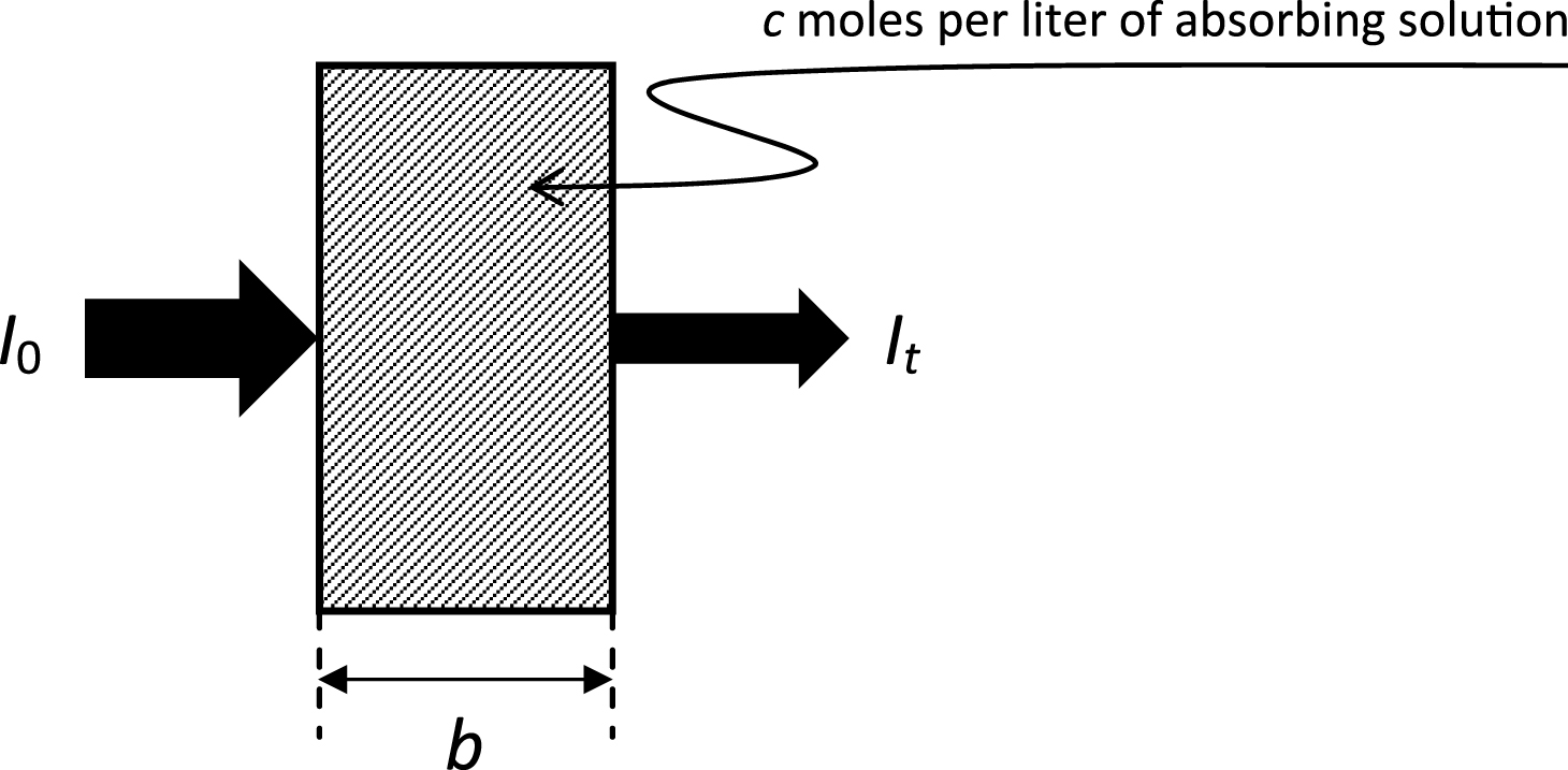
Fig.2
Each element of the mesh yields a unique set of regression equations.
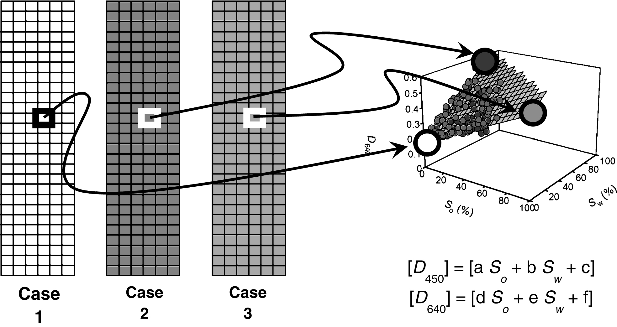
Fig.3
Grain size distribution of Toyoura sand.
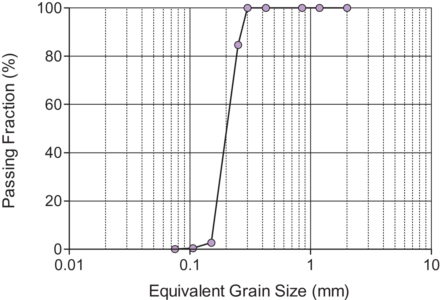
Fig.4
Column system design.
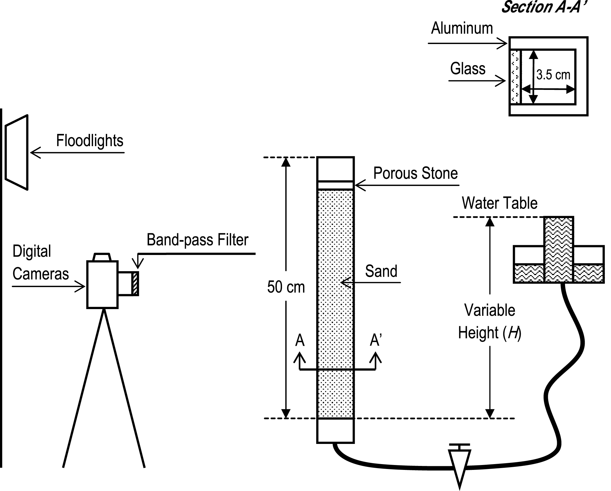
Fig.5
Picture Setup for the Saturation-Optical Density Relationship Test.
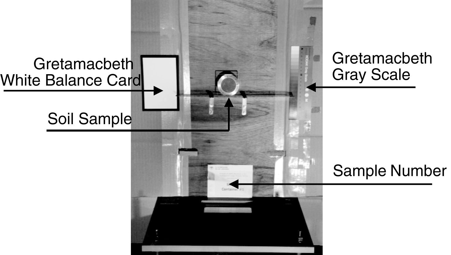
Fig.6
Transmittance graphics for a. Ethylbenzene; b. Low viscosity paraffin; c. Motor oil; d. N-Decane; e. N-Dodecane; f. NEOVAC; g. Nitrobenzene; h. Silicone oil; i. Diesel 2.
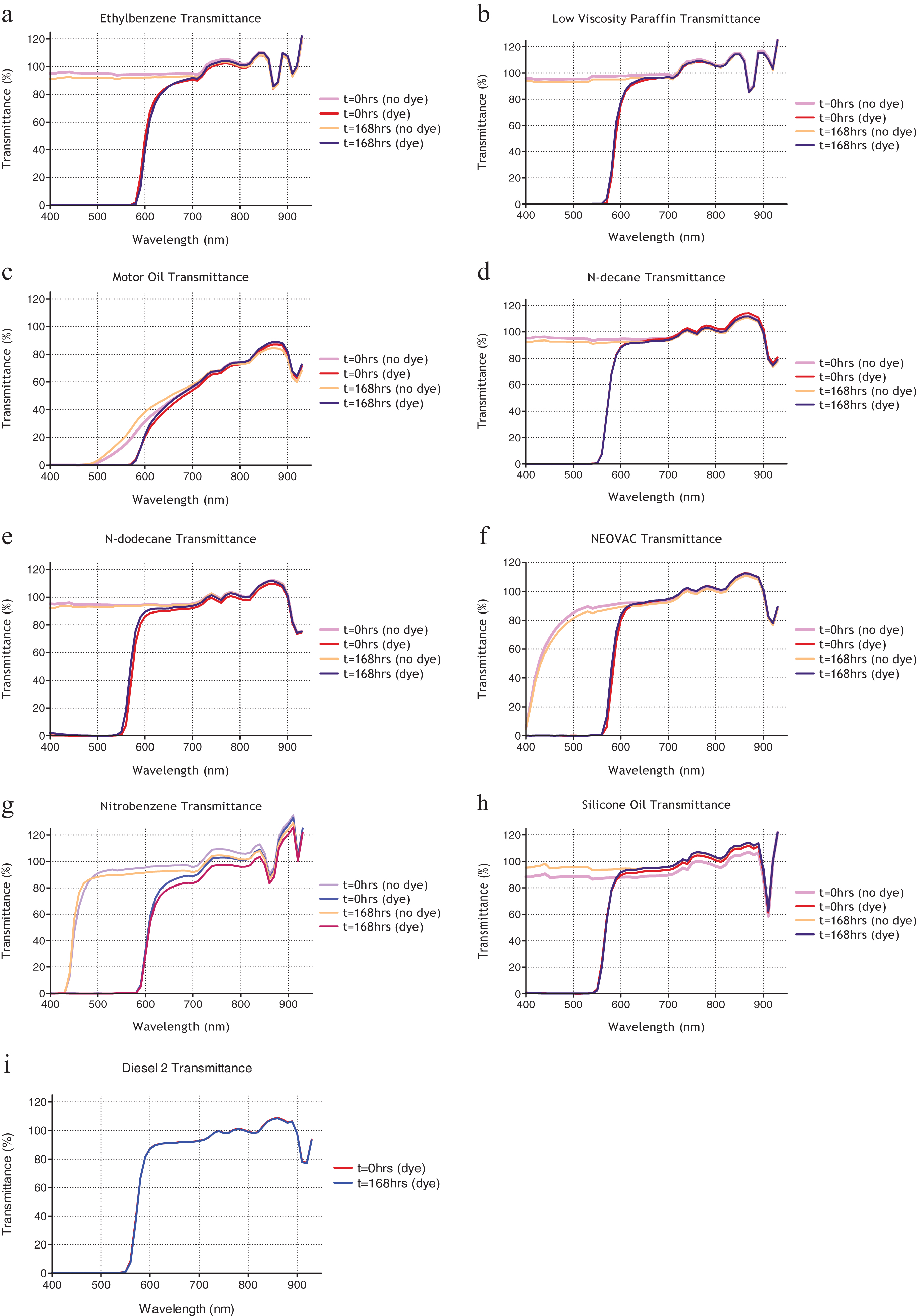
Fig.7
Saturation vs. Optical Density for Motor Oil, at wavelength: a. Standard view 450 nm; b. Orthogonal view 450 nm; c. Standard view 640 nm; d. Orthogonal view 640 nm.
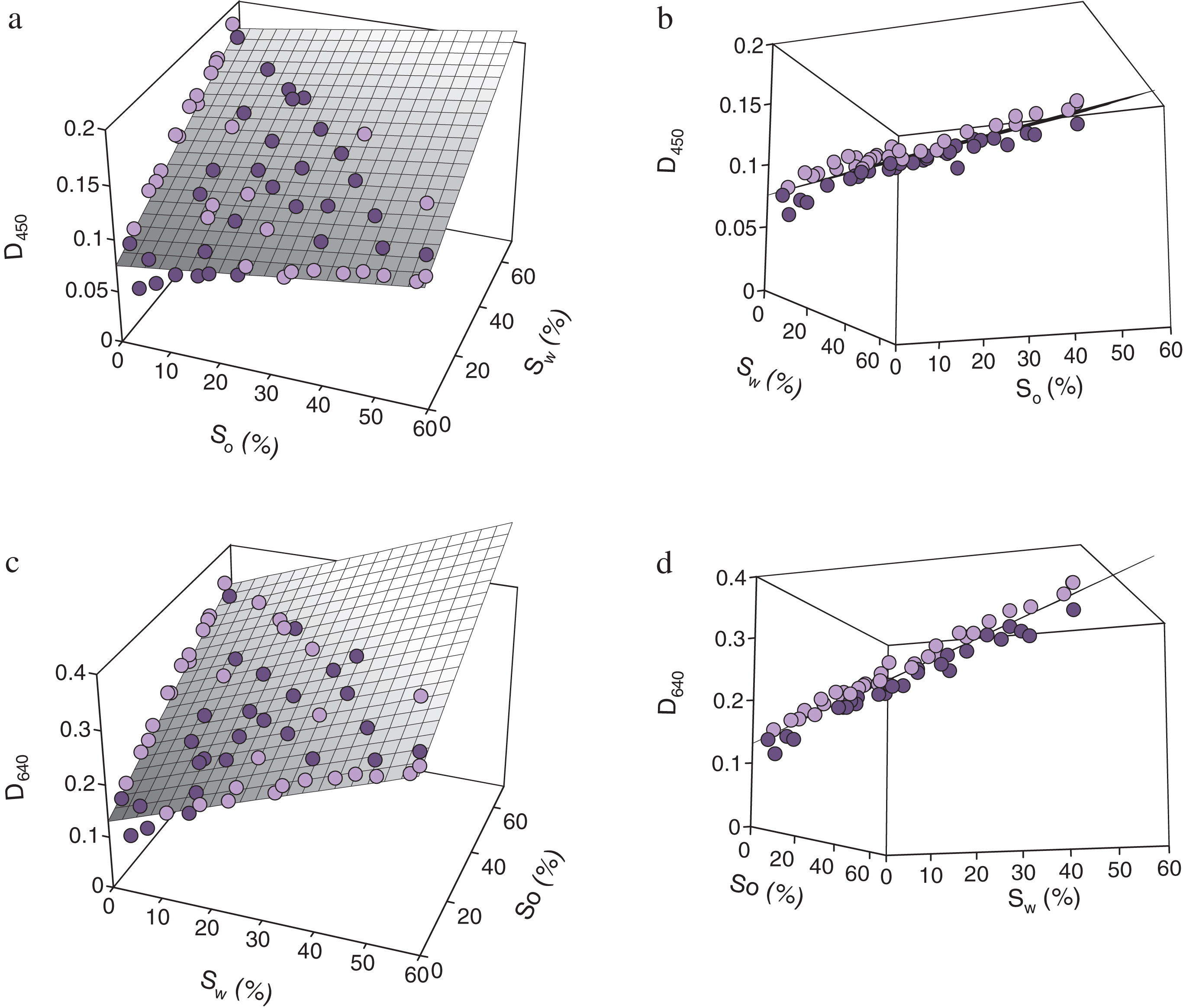
Fig.8
LNAPL saturation (a) and water saturation (b) changes with time, at different heights, for ethylbenzene.
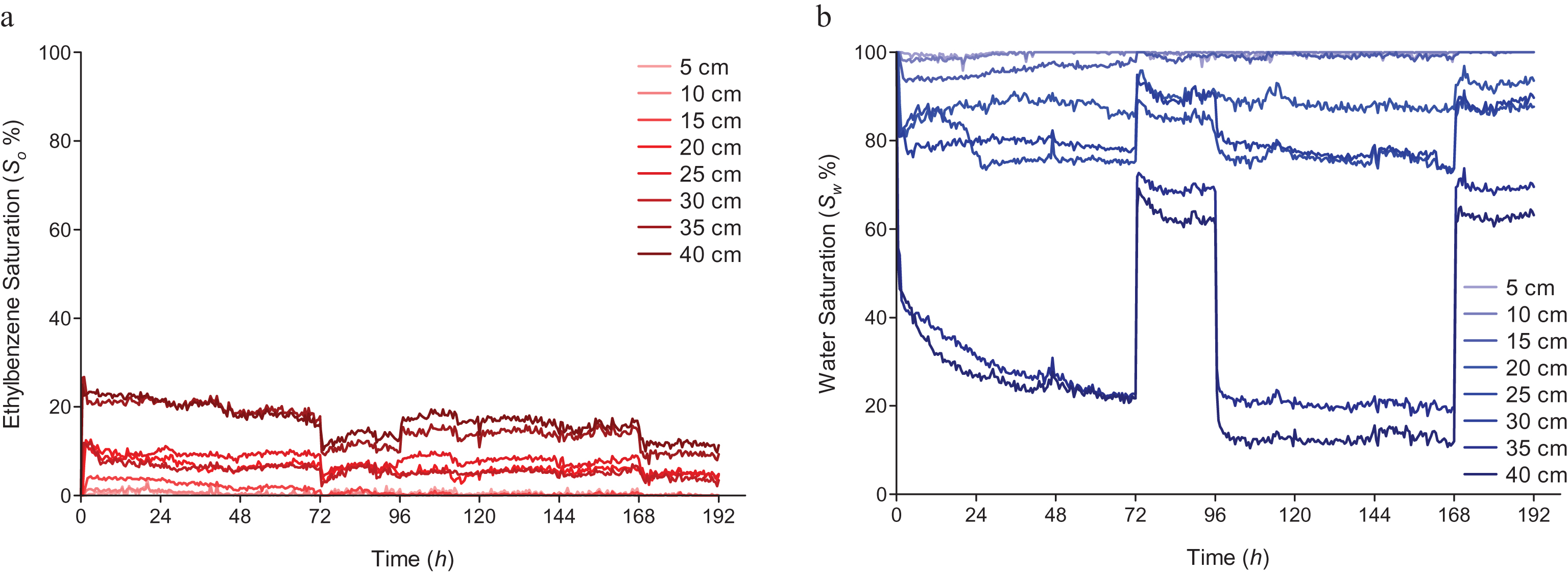
Fig.9
LNAPL distribution during the first drainage (t = 0–12 h), for ethylbenzene. Fringe of the mobile fraction is shown.
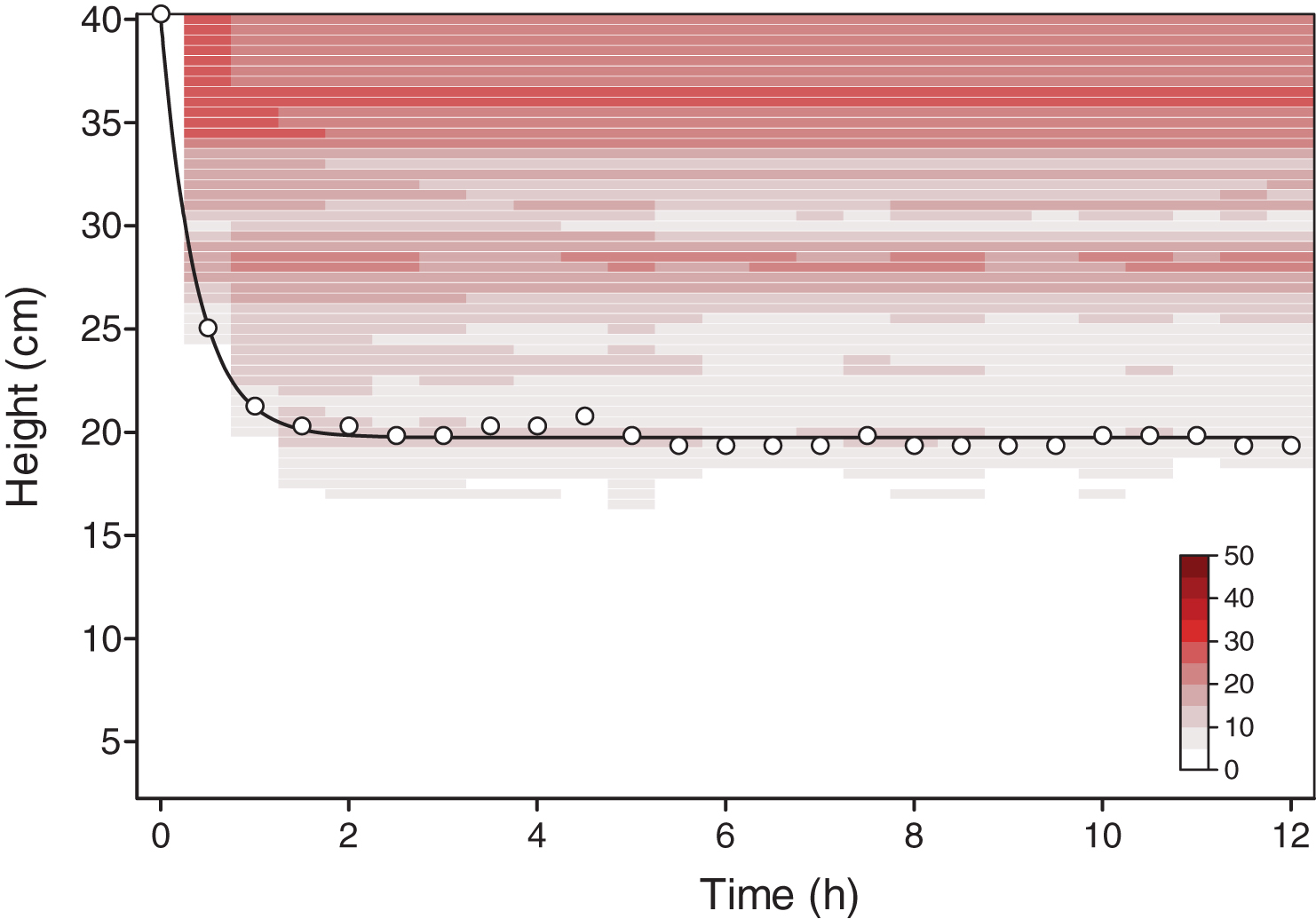
Fig.10
Mobile fraction of four LNAPLs during the first 12 hours of a. First drainage; b. First imbibition; c. Second drainage; d. Second imbibition.
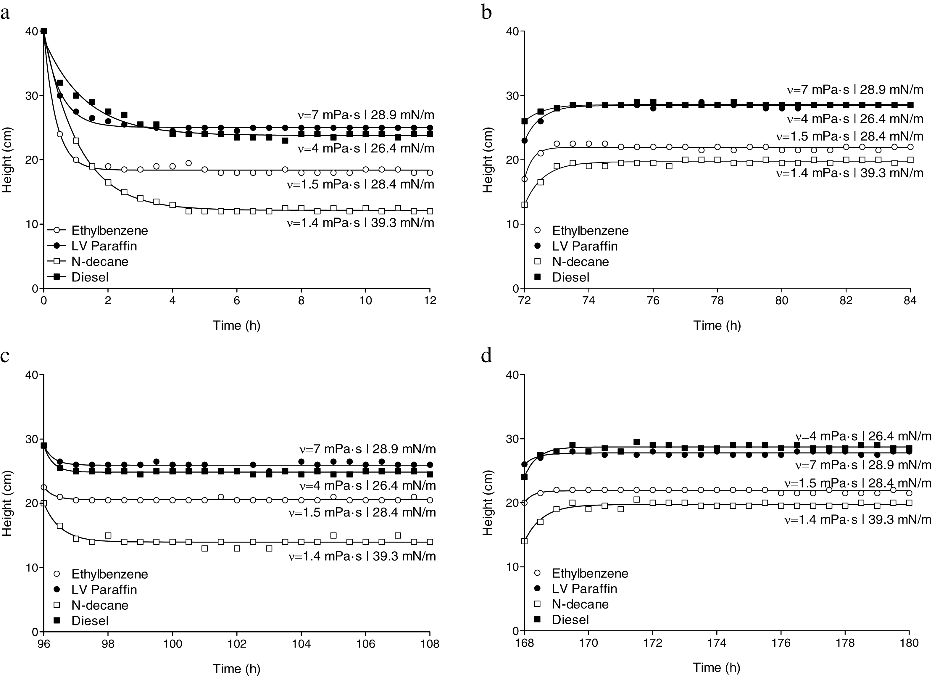
Fig.11
Comparison of the mobile fraction during the first 12 hours of each drainage and imbibition processes a. Ethilbenzene; b. N-decane; c. Low viscosity paraffin; d. Diesel 2.
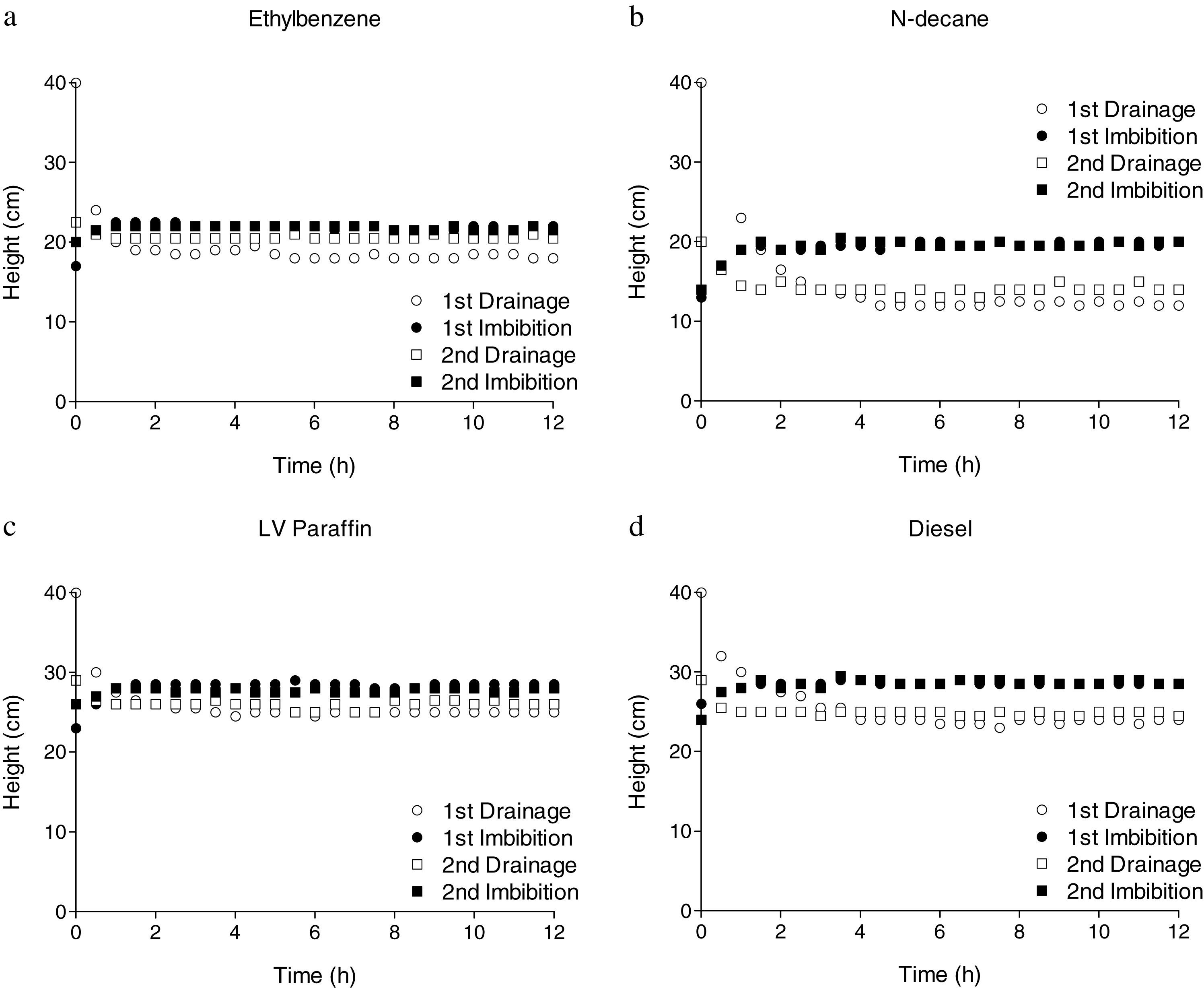
Fig.12
Relation between interfacial tension (NAPL/water) and the difference in depth of the mobile fraction between the first drainage and imbibition stages.
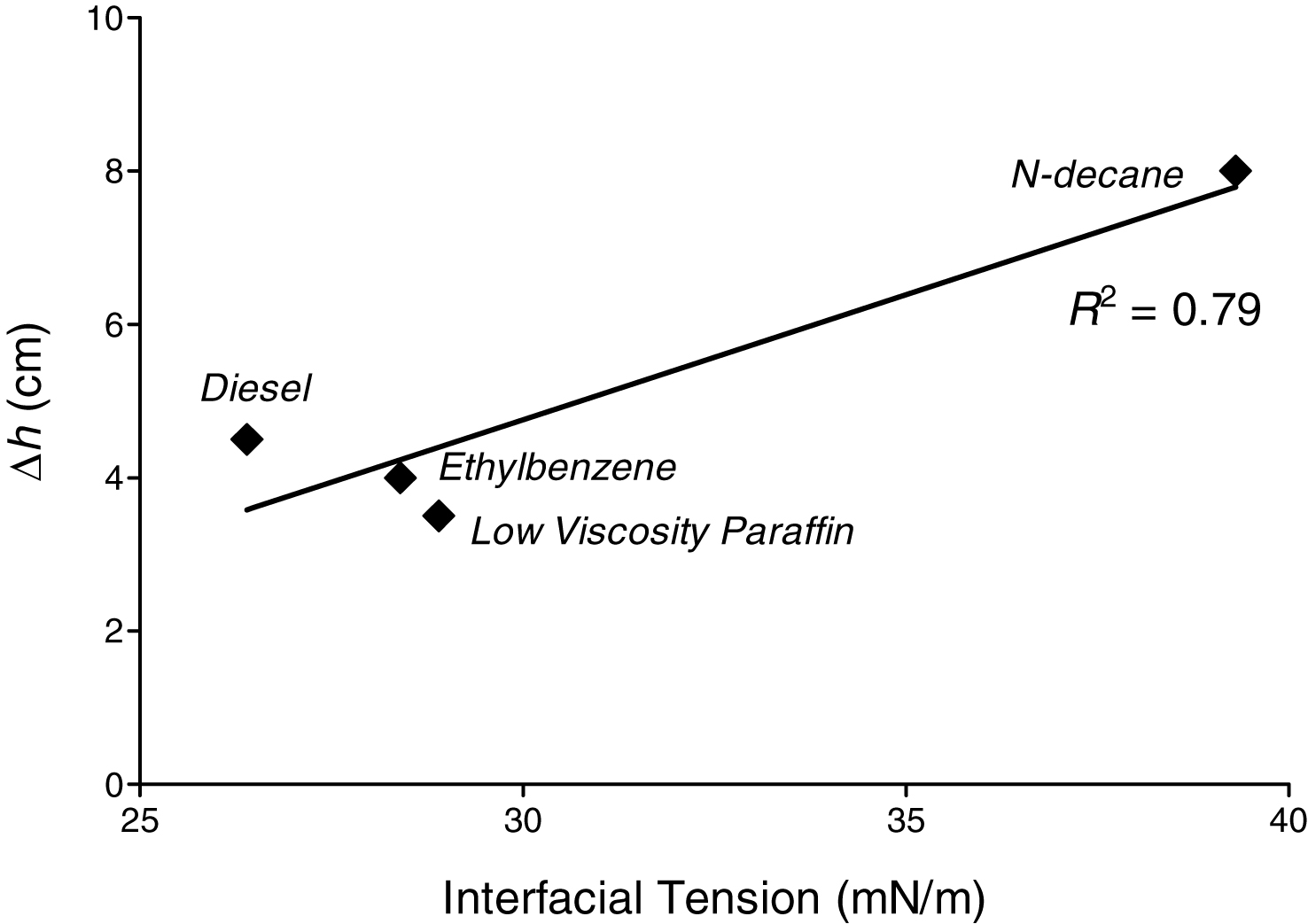
Fig.13
Relation between viscosity and depth of the mobile fraction for different LNPALs.
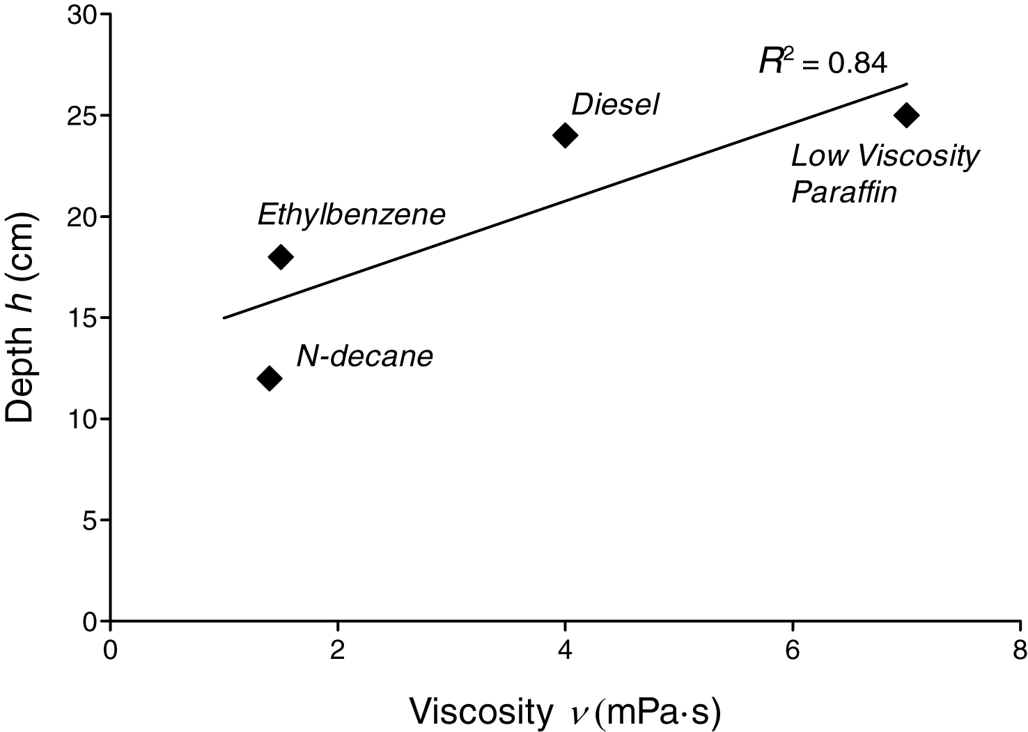
Fig.14
Comparison of residual saturation at the end of drainage and imbibition stages for 5 different NAPLs (left) and relationship between their viscosity and imbibition/drainage saturation ratio (right).
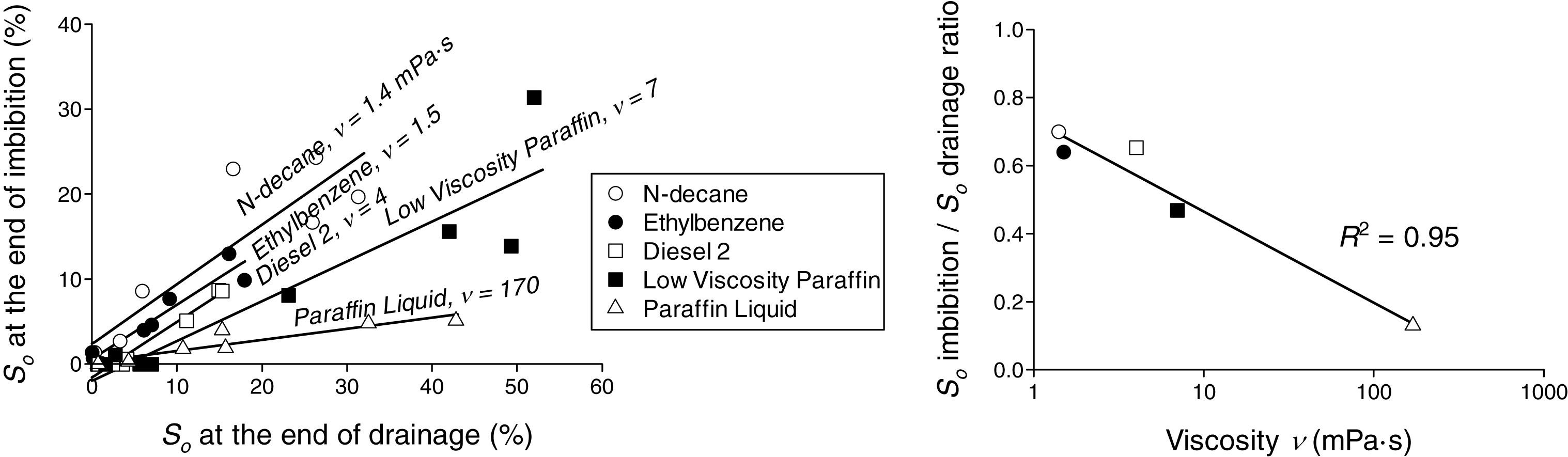
Table 1
Physical characteristics of used NAPLs
| NAPL | Solubility in Water | Density ρ (g/cm3) | Viscosity ν (mPa · s) |
| Ethylbenzene | 0.0169 g/l | 0.860 | 1.5 |
| Low Viscosity Paraffin | Immiscible | 0.880 | 7 |
| Motor Oil | Immiscible | 0.858 | 129 |
| N-Decane | 0.009 ppm | 0.730 | 1.4 |
| N-Dodecane | Immiscible | 0.750 | 1.9 |
| NEOVAC | Negligible | 0.930 | 108 |
| Nitrobenzene | 0.019 g/l | 1.199 | 3.1 |
| Silicone Oil | Negligible | 0.963 | 1000 |
| Diesel 2 | Immiscible | 0.850 | 4 |
Table 2
Regression equations for different NAPLs, for wavelengths λ= 450 nm and 640 nm
| NAPL | D450 | R2 | D640 | R2 |
| Ethylbenzene | 0.0175 So + 0.0007 Sw + 0.0680 | 0.81 | 0.0033 So + 0.0037 Sw + 0.1220 | 0.90 |
| LV Paraffin | 0.0160 So + 0.0008 Sw + 0.0710 | 0.89 | 0.0029 So + 0.0036 Sw + 0.1300 | 0.93 |
| Motor Oil | 0.0150 So + 0.0006 Sw + 0.0750 | 0.91 | 0.0028 So + 0.0033 Sw + 0.1300 | 0.92 |
| N-Decane | 0.0150 So + 0.0008 Sw + 0.0700 | 0.89 | 0.0033 So + 0.0040 Sw + 0.1200 | 0.96 |
| N-Dodecane | 0.0160 So + 0.0007 Sw + 0.0700 | 0.88 | 0.0030 So + 0.0035 Sw + 0.1300 | 0.95 |
| NEOVAC | 0.0140 So + 0.0008 Sw + 0.0700 | 0.85 | 0.0025 So + 0.0036 Sw + 0.1300 | 0.95 |
| Nitrobenzene | 0.0130 So + 0.0007 Sw + 0.0730 | 0.85 | 0.0026 So + 0.0036 Sw + 0.1300 | 0.94 |
| Silicone Oil | 0.0120 So + 0.0009 Sw + 0.0690 | 0.93 | 0.0023 So + 0.0040 Sw + 0.1200 | 0.97 |
| Diesel 2 | 0.0180 So + 0.0035 Sw + 0.2457 | 0.83 | 0.0030 So + 0.0025 Sw + 0.1283 | 0.95 |
Table 3
Depth of mobile fraction of different LNAPLs after first drainage, and time to reach a stable condition
| LNAPL | Viscosity ν (mPa · s) | Depth (cm) | Time (h) |
| Ethylbenzene | 1.5 | 18.0 | 2 |
| LV Paraffin | 7 | 25.0 | 3 |
| N-decane | 1.4 | 12.0 | 5 |
| Diesel | 4 | 24.0 | 6 |


