
A practical approach for the consideration of single pile and pile group installation effects in clay: Numerical modelling
Abstract
In this paper, a practical approach for the consideration of single pile and pile group installation effects in clay is presented using some novel procedures implemented in the finite element (FE) software package PLAXIS 2D. Data reported at a soft clay site at Islais Creek, San Francisco are used to provide calibration for the constitutive model and to validate initial predictions of single pile installation effects. A short parametric study was then undertaken to examine the influence of a number of pile/soil parameters on the soil stresses generated around a single pile after installation and subsequent consolidation. In addition, a new simplified method is proposed to consider group installation effects over-and-above those associated with an equivalent single pile involving the volumetric expansion of tunnels within a plane-strain framework. Remarkably, results show that the installation of additional group piles has a negligible influence after consolidation.
1Introduction
Over the last several decades, numerous investigators have endeavoured to provide a more complete understanding of the processes associated with soil disturbance during pile installation and subsequent consolidation in clays. The cavity expansion method (CEM; [1–3]) and strain path method (SPM; [4]) are amenable to immediate use by design engineers and for that reason have been to the forefront of the mathematical approaches used to model pile installation. CEM has the advantage over SPM in that coupled consolidation analyses require SPM to be paired with FE analyses for the consolidation process; this involves interpolation of stresses, pore pressures and hardening parameters from the SPM mesh to the FE mesh and does not lend itself easily to parametric studies [5]. CEM therefore provides a more versatile tool for conducting parametric studies of both short-term and long-term pile installation effects.
Butterfield and Banerjee [6] provided the first comprehensive application of cylindrical CEM to the investigation of installation effects along a pile shaft in clay. The Effective Stress Axial Capacity Cooperative (ESACC) program led to the development of four generations of effective stress soil models (ESM1 to ESM4) for improved predictions of installation-induced changes in soil stresses using CEM; this ultimately led to the development of the axi-symmetric radial consolidation program CAMFE [3]. This coupled finite element formulation has been used to simulate the installation of a pile in clay and subsequent dissipation of excess pore pressures using cylindrical CEM (e.g. Randolph et al. [7]). Heydinger and O’Neill [8] later improved upon the work carried out by the ESACC research group and developed the finite element (FE) program VECONS which empirically considered the soil in the plastic zone surrounding the pile to have anisotropic stiffness during consolidation. Following these developments, further FE solution procedures were adopted to analyse the cavity expansion problem (e.g. 9–11). Collins and Stimpson [9] used similar solutions to investigate the expansion of a cavity of zero radius in hardening/softening soils for both drained and undrained conditions using the MCC model. Cao [10] and Cao et al. [11] applied cylindrical CEM to a linear elastic MCC material while Cao et al. [12] later extended the approach to the case of soil stiffness nonlinearity. More recently, Lehane and Gill [13] reported good agreement between CEM predictions and measured radial displacements induced during the installation of six separate closed-ended pipe piles in clay.
In this paper, a practical approach for the consideration of single pile and pile group installation effects in clay is presented using the FE software package PLAXIS 2D, Version 2012.0 [14]. The advanced MIT-S1 constitutive model is employed to investigate the effects associated with the installation of a single pile using an adaptation of the traditional cylindrical CEM analysis where vertical displacements are imposed simultaneously with the expansion of the cavity. The present study is associated with friction piles and therefore installation effects below the base of the pile are outside the scope of this paper; henceforth CEM refers to the expansion of a cylindrical cavity. Data reported at a soft clay site at Islais Creek in San Francisco (supplemented by data from other nearby test sites) is used to provide calibration for the constitutive model and to validate initial predictions of single pile installation effects. A short parametric study is conducted to investigate the influence of a number of pile/soil parameters on long-term stresses set up in the soil after pile installation and subsequent consolidation of excess pore pressures.
The well-documented MCC model is employed to consider the more computationally-intensive analysis of additional group effects. To date, no numerical investigations have been conducted on the installation effects of piles in groups since CEM cannot be applied to these analyses without simplifying the group to an equivalent pier. A new simplified method is therefore proposed to consider group installation effects over-and-above those associated with an equivalent single pile involving the volumetric expansion of tunnels within a plane-strain framework.
2Pile installation programme in Young Bay Mud
2.1General site characterization
Field data from the pile installation research reported by Pestana et al. [15] and Hunt et al. [16] are used to appraise the simplified methods for predicting installation effects in this paper. The project site is located at Islais Creek on the San Francisco Peninsula in California. The site exploration for this project consisted of two seismic cone penetration (SCPTu) tests and eight borings. The ground profile consists of a layer of fill which extends to a depth of approximately 3.5 m, a deep deposit comprising two layers of Young Bay Mud (YBM) from 3.5 m – 31 m which are separated by a stiffer and significantly more permeable layer at a depth of approximately 15.5 m–17.5 m. YBM is a soft, moderately sensitive marine clay and its properties have been the subject of much investigation at UC Berkeley over the past couple of decades. The summary properties of the YBM are given in Table 1 [16]. A stratum of stiff sand exists at 31 m below ground level and piezometer measurements give an approximate ground water table at a depth of 2.1 m.
2.2Details of instrumentation and pile installation
The pile used in the project was a 610 mm diameter (D), 12.7 mm thick and 36.6 m long closed-ended steel pipe pile. The project consisted of a total of 10 boreholes as shown in Fig. 1. Instrumentation included pneumatic piezometers which were installed at depths of 8.5 m and 12.8 m at three nominal distances from the pile-soil interface, labeled B-1, B-2 and B-3, and three inclinometer casings with single piezometers below each, at a depth of 23.8 m and labeled B-4, B-5 and B-6. Nominal distances are approximately 0.90D, 1.90D and 3.39D for B-1, B-2 and B-3, respectively and 1.24D, 2.13D and 3.61D for B-4, B-5 and B-6, respectively, where D is the pile diameter.
3Constitutive soil models and parameters
3.1MIT-S1
The generalised effective stress model MIT-S1 was adopted in the present study to simulate the stress-strain-strength properties of San Francisco YBM. The MIT-S1 model describes the rate independent behaviour of freshly-deposited and overconsolidated soils and its formulation is based on the incrementally linearized theory of elasto-plasticity. Further information on the formulation of the model is available in [17].
The MIT-S1 model requires the input of 13 soil parameters for clays which can be obtained from standard laboratory tests [18]. The MIT-S1 parameters adopted in the present study are presented in Table 2 for depths of 8.5, 12.8 and 23.8 m together with their physical meaning. Although the parameters presented in this paper are intended to be a representation of the Islais Creek test site, insufficient data for the calibration of certain model parameters to this particular site necessitated that the data reported by Hunt [19] were supplemented with data from alternative nearby test sites as illustrated in Fig. 2.
Compression coefficients, ρ c , for YBM were calculated from the slope of the normal compression line (NCL) in a double logarithmic void ratio-effective stress space from oedometer tests reported by Hunt [19] for a depth of ∼8.5, ∼12.8 and ∼23.8 m, respectively. The parameters D and r describe the hysteretic volume response. Values of D were selected by measuring the slope of the unloading curve at an overconsolidation ratio (OCR) ≥ 10 while values of r were selected from curve-fitting to the unloading stress-strain behaviour in a standard oedometer test documented by Hunt [19] as shown in Fig. 3. The parameter h controls the amount of normalised irrecoverable plastic strain observed in unload-reload cycles and was again selected by curve-fitting to the oedometer test data reported by Hunt [19]. The fit between measured data and calibrated predictions are shown in Fig. 3 for all three depths.
The MIT-S1 model uses a variable μ′ to account for the variation in K 0 during one-dimensional loading and unloading according to the following relationship [18]:
(1)
(2)
Figure 5 shows plots used to calibrate the parameters
The parameter ψ controls the amount of rotational hardening and is best calibrated to CK0UE measured stress paths [18]. To the authors’ knowledge, there are no CK0UE measured stress paths for YBM documented in the literature. Instead, the authors employed measured CK0UE stress-strain curves documented by Duncan [21] for the purpose of refining the value of ψ for YBM as shown in Fig. 6.
Small strain non-linearity in shear is controlled by the parameter ω s and was chosen by curve-fitting to the shear modulus degradation curves reported by Hunt [19] in Fig. 7. This data is also supplemented with data reported by Stewart and Hussein [20] and Sitar and Salgado [22].
The parameter C b controls the small strain elastic shear and bulk modulus and was obtained using the following closed-form equation [23]:
(3)
In order to validate the adopted model parameters outlined in the preceding section, the MIT-S1 model was used to predict the stress-strain curves and pore pressures in undrained triaxial compression documented by Hunt [19]. In Fig. 9, it can be seen that MIT-S1 predictions agree well with measured data consolidated to both pre-pile in-situ stresses and to three times pre-pile in-situ stresses. Similarly, the MIT-S1 predictions appear to be in good agreement to measured pore pressures in Fig. 10. Thus from Figs. 9 and 10, the selected model parameters can be considered a satisfactory representation of the behaviour of YBM at the Islais test site.
3.2Modified Cam-Clay
In this study, the MIT-S1 constitutive model was employed as a user-defined dll and was therefore not optimised within the FE code which limited its use to more routine analyses. It was therefore not feasible to consider group effects with this model and the extensively-employed MCC constitutive model was adopted for this purpose. In PLAXIS, the MCC soil model requires five input parameters, listed in Table 3 together with their physical meaning. The MCC parameters at a depth of 12.4 m were chosen for the purpose of undertaking the parametric study on the influence of pile group installations.
Commonly used relations were used to develop MCC parameters from the one dimensional consolidation tests, as opposed to the isotropic consolidation tests that form the basis of the model. Thus, Cc and Cr reported by Hunt [19] were used to determine λ, and κ from:
(4)
(5)
Fig. 11a shows the plot used to calibrate the MCC model versus laboratory consolidated undrained triaxial tests at the depth of 12.4 m. As MCC could not match the strain-softening behaviour of YBM, a value of M was targeted at the peak deviator stress for the test. A value of OCR = 1 was adopted for the simulation of this test as mentioned in the previous section.
As shown on the Fig. 11b and 11c, the selected MCC parameters lead to reasonable approximations of the failure stresses and strains, but fail to capture post-peak decreases in deviatoric stress and increases in pore pressure. Thus, when interpreting results from PLAXIS with the MCC soil model, it is important to recognize that for soil regions close to the pile, which will be strained well beyond peak strength, stresses will likely be overpredicted and pore pressures underpredicted.
4Details of finite element modelling
4.1Modelling single driven piles using CEM
In this paper, predictions of pile installation-induced changes in the soil are obtained using CEM in PLAXIS 2D. In the literature to date, predictions of installation and equilibrium stresses at the pile shaft evaluated by the CEM are limited to the consideration of lateral deformations and do not take into account vertical deformations due to pile installation. However, Ni et al. [24] made use of transparent soil and particle image velocimetry (PIV) to study the 3-D movement of clay during pile penetration; those authors illustrated the accumulated displacement vectors after pile installation. The measured movement of the soil for a normalized radial distance of r/R<1 could not be shown and thus a value of r/R = 2 represents the lower bound limit for the measurements in that study. At r/R = 2, the value of z/R varied from 2 (at the pile base) to approximately 1 mid-way up the shaft where z is the vertical component of the soil displacements. On the basis of those findings, both vertical and radial displacements are imposed simultaneously in this study to simulate more realistic soil movement after pile installation (see Fig. 12). The extent of vertical deformations are considered by imposing a value of z/R (which is varied in the present paper) where a value of z/R = 0 replicates a traditional CEM analysis; this approach somewhat resembles the approach adopted by Broere and Van Tol [25] for the investigation of the bearing capacity of a bored pile in sand.
Gavin et al. [26] noted that long-term friction fatigue effects of piles installed in a soft estuarine clay were negligible largely due to the undrained nature of pile installation which prevented appreciable volume change occurring. Since pile loading typically occurs after sufficient dissipation of excess pore pressures, the omission of friction fatigue effects in this study was deemed a reasonable simplification.
The stages used in the simulation of pile installation are defined as follows:
(i) Initial stress generation by the K 0 procedure, a special calculation method available in PLAXIS.
(ii) Installation of ‘dummy material’ over the entire pile length to a radial extent, a 0.
(iii) Application of a prescribed radial displacement from the initial radius, a 0, to a final radius, a f (corresponding to the pile radius, R), while simultaneously prescribing a vertical displacement z at the pile-soil interface to obtain the chosen value of z/R.
(iv) Pore pressure equalisation to establish the long-term stress changes in the ground caused by pile installation.
In all analyses, the FE mesh was refined in zones of high stresses near the pile as shown in Fig. 13; also shown is the mesh deformation for a value of z/R = 2. Geometric nonlinearity was included to account for the large deformations. The depth of the pile was chosen equal to 5 m; similarly the depth of the FE model was chosen equal to 7 m. Roller supports were used at the bottom boundary to allow lateral movement while the lateral boundaries of the model were fixed.
4.2Pile group installation - Volumetric Tunnel Expansion (VTE)
To date, pile group installation effects have not been considered within a numerical framework in the literature for two main reasons: [1] 2-D analyses are not capable of modelling additional group piles in discrete locations (an annular ring is generated instead) and thus CEM analyses are not applicable and [2] although 3-D FE analyses are capable of considering pile groups in PLAXIS, these are based on small strain theory and cannot accommodate large deformations.
In the present study, a new simplified method has been adopted in order to consider the effects of piles installed in a group. This analysis involves the expansion of a tunnel in conjunction with a plane strain model in PLAXIS. This method is referred to as volumetric tunnel expansion (VTE) henceforth because it uses the tunnel designer in PLAXIS distinguishing it from the conventional analyses involving the expansion of a cylinder of soil using an axi-symmetric model.
Using this method, Fig. 14 is now considered as a plan view of a 9-pile group at a particular elevation in the soil as opposed to the conventional elevation view. Therefore in these analyses the z-direction is no longer considered vertical but on the horizontal plane normal to the x-direction. In order to have symmetry in the x and z directions, a value of lateral earth pressure, K, equal to 1 was used to ensure
The stages used in the simulation of pile group installation by this method are defined as follows:
(i) Initial stress generation by the K 0 procedure.
(ii) Installation of ‘dummy material’ over pile area with radius a 0.
(iii) Application of a percentage volumetric strain (undrained conditions) to the pile areas simultaneously until a radius a f is reached.
(iv) Pore pressure equalisation to establish the long-term stress changes surrounding the pile group.
The authors concede that in practice all piles within a group are not installed concurrently but in a sequence usually beginning at the centre of the group and moving radially outwards, or beginning at one corner and progressing towards the opposite corner. The time taken to install a typical pile, however, is generally substantially less than the time taken for significant pore pressure dissipation to occur in low permeability soils; thus the authors do not believe this simplification to have an appreciable influence on results.
5Comparison of CEM single pile predictions to measured data
5.1Pore pressures
While Hunt [19] reported an OCR of between 1.2 and 1.4, a value of OCR = 1.2 was adopted for the three depths in this section; given the uncertainty in the determination of OCR from consolidation tests, this was not considered an unreasonable adjustment [19]. In Fig. 15, pore pressures estimated using the MIT-S1 model in PLAXIS (using a value of z/R = 2) have been compared to measured data documented by Hunt [19] at depths of 8.5 m (Fig. 15a), 12.8 m (Fig. 15b) and 23.8 m (Fig. 15c), respectively, at the Islais Creek test site.
Measured values of pore pressures are shown on the plot with circles at the normalised radial distances corresponding to the base of the inclinometer casings in addition to 2% error bars corresponding to the uncertainty in the location of the piezometers. For the 23.8 m depth, Hunt [22] corrected the normalised radial distances to the measured pore pressures by back-calculating the lateral deformations using CEM and these have also been presented in Fig 15c. It can be seen from Figs. 15a-15c that, in general, CEM predictions with z/R = 2 and in conjunction with the MIT-S1 model provide good agreement to measured data for all three depths.
5.2Deformations
In Fig. 16, measured values of radial displacement at the end of pile installation and after consolidation (i.e. 678 days) are shown with corresponding PLAXIS predictions for a depth of 12.8 m. It can be seen from Fig. 16 that PLAXIS predictions show good agreement to the measured deformations after pile installation for all three radial locations.
5.3Shear wave velocities
The well known relationship defined in Eq. 6 has been employed to convert variations in shear wave velocities to variations in shear modulus where V s is the current shear wave velocity, V s0 is the far-field (undisturbed) shear wave velocity, G is the current soil shear modulus, G 0 is the far-field (undisturbed) soil shear modulus.
(6)
It is obvious that a variation in V s will have a significantly larger difference than a variation in ρ; thus the variation in ρ of the soil has been neglected (ρ/ρ 0 assumed equal to 1). Furthermore, the shear modulus of the soil can be related to the mean effective stress (which can be obtained from FE output) according to the following relationship:
(7)
where p′ is the current mean effective stress in the soil,
6Long-term stress changes around a single pile
6.1Influence of pore pressure dissipation
In Fig. 18, lateral variations in normalised soil stresses
Predictions of Δu/s
u
reported by Randolph [28] using simple cavity expansion theory (z/R = 0) applied to an elastic perfectly plastic soil have been superimposed on Fig. 18a; a value of
It can be seen from Fig. 18b that there is an increase in the value of
6.2Influence of OCR
In Figs. 19a and 19b the influence of OCR on the lateral distribution of
6.3Influence of soil type
In Figs. 20a and 20b, the influence of soil type on predictions of
6.4Influence of constitutive model
As mentioned previously, and presented in the following section, the authors have adopted the MCC soil model for the purpose of evaluating pile group installation effects. Prior to pile group analysis, the results of single pile long-term stresses evaluated using CEM in conjunction with the MCC and MIT-S1 have been compared in Fig. 21. It can be seen that the numerical noise is eliminated when using the MCC model which is available within the commercial version of PLAXIS. Since the MCC will be used for investigating pile group installation effects, only comparisons at realistic pile spacings are made in Fig. 21 i.e. r/R>5. It can be seen that MCC gives reasonable predictions of
7Pile group installation effects
7.1Comparison of single pile predictions
In order to consider the influence of piles installed in a group, the authors adopt the VTE method outlined in Section 4.2. In Figs. 22a and 22b, predictions of single pile installation stresses after pile installation and after consolidation evaluated using VTE have been compared to traditional CEM predictions (with z/R = 0). Measured data documented by Hunt [22] and data from a single pile installed in Belfast estuarine silt reported by McCabe et al. [29] have also been included in Fig. 22a; although comparison to the latter is only indicative since different soil parameters have been adopted, both sets of data show good agreement. At realistic pile spacings (i.e. r/R > 5), predictions evaluated by VTE show surprisingly better agreement to field data. Moreover, predictions of
From the results presented in Fig. 22, it can be deduced that the VTE method gives reasonable predictions compared to traditional CEM predictions for r/R > 5, i.e. at locations of neighbouring groups piles; therefore only group installation effects over-and-above those owing to each pile’s own installation is considered in the subsequent sections.
7.2Group effects after installation
The authors have adopted the conventional
A cross-section was taken through the group as shown for N = 9 group in Fig. 24 to examine the lateral distribution of soil stresses. In Fig. 25, the lateral distribution of excess pore pressures surrounding a single pile have been compared to that existing within a group with N = 9, 25 and 49 for a pile spacing-to-diameter (s/D) ratio of 3. The origin of the single pile predictions has been located at the centre of each group; therefore it is only the agreement between the group and single pile predictions in the vicinity of the centre pile that is sought from these comparisons.
For the sake of clarity and to isolate the effect of the additional group pile installations better, the group distributions have been normalized by the single pile predictions and have been re-plotted in Fig. 26a on a log-log scale where Δu G is the excess pore pressure distribution within the groups, Δu S is the excess pore pressure distribution surrounding an equivalent single pile and a value of Δu G /Δu S = 1 indicates zero group effects. Measured excess pore pressures of a model 5-pile group in estuarine silt reported by McCabe et al. [29] in addition to measurements reported by O’Neill et al. [30] in a stiff overconsolidated clay are also superimposed on the graph for comparative purposes. It can be seen that present predictions and measured data show remarkably good agreement for 1 ≤r/R ≤15. In addition, it is clear that group effects do not cause an appreciable increase in excess pore pressures at the centre group pile. While Δu G /Δu S is an expedient measure of additional group effects, for larger values of r/R (i.e.>15), Δu S becomes very small and therefore the value Δu G /Δu S becomes less reliable; the authors therefore attribute the difference between the numerical predictions and measured data at r/R>15 to this effect.
In Fig. 26b, an increase in
7.3Group effects after consolidation
In Fig. 27a, the variation in
In Fig. 27b, the influence of the pile spacing-to-diameter (s/D) ratio on group installation effects is examined. It can be seen that the value of s/D has a negligible influence on group effects experienced in the vicinity of the centre group pile; however, an increase in the value of s/D results in a value of
8Conclusions
In this paper, a comprehensive numerical study on single pile and pile group installation effects in clay has been presented. The advanced MIT-S1 constitutive model was employed to investigate the effects associated with the installation of a single pile using a modified version of the CEM method while the extensively-employed MCC model was employed to consider the more computationally-intensive investigation of additional group effects. The authors have arrived at the following conclusions arising from the study:
(i) A variation on the traditional CEM method was adopted where vertical displacements were imposed concurrently with the expansion of the cylindrical cavity. Predictions of soil stresses and excess pore pressures after pile installation and during subsequent dissipation of said pore pressures showed good agreement to measured data documented by Hunt [19] in San Francisco YBM.
(ii) The well-known MCC clay model was adopted to consider the influence of group effects since the parametric study with MIT-S1 as a user-defined soil model was not feasible. Comparisons between the MCC and MIT-S1 models showed good agreement at practical pile spacings and was deemed suitable for the investigation of group effects over-and-above those owing to each pile’s own installation.
(iii) The authors proposed a new simplified method using the expansion of tunnels within a plane-strain framework for the consideration of group installation effects. Single pile predictions determined using this method after installation showed good agreement to traditional CEM predictions (with z/R = 0) in addition to measured field data.
(iv) Moreover, it was shown that after the installation of a pile, the installation of additional neighbouring piles do not influence the excess pore pressures near the pile-soil interface. In contrast, however, significant increases in both radial effective stress and mean effective stress were noted near the pile-soil interface with N = 9, 25 and 49.
(v) After consolidation, all group effects diminished, supporting the findings of McCabe [31] who noted that the additional group effects associated with a model 5-pile group installed in clay were transient.
ACKNOWLEDGMENTS
The first author gratefully acknowledges the College of Engineering and Informatics, NUI Galway, and the University of California Education Abroad Program for funding this research. In addition, the authors gratefully acknowledge the GeoEngineering department at Massachusetts Institute of Technology who compiled and provided the authors with the MIT-S1 dll for this research.
References
1 | Gibson RE, Anderson WF(1961) In-situ measurement of soil properties with the pressuremeterCivil Engineering and Public Works Review56: 658615618 |
2 | Vesic AS(1972) Expansion of cavities in infinite soil massJournal of the Soil Mechanics and Foundations Division, ASCE98: SM3265290 |
3 | Carter JP, Randolph MF, Wroth CP(1979) Stress and pore pressure changes in clay during and after the expansion of a cylindrical cavityInternational Journal for Numerical and Analytical Methods in Geomechanics3: 305322 |
4 | Baligh MM(1985) Strain path methodJournal of Geotechnical Engineering, ASCE111: 911081136 |
5 | Perri JF(2007) Assessment of capacity and seismic demand on axially loaded piles in soft clayey deposits [Ph.D. Thesis]University of California, BerkeleyCA |
6 | Butterfield R, Banerjee PK(1970) The effect of porewater pressures on the ultimate bearing capacity of driven piles2nd Southeast Asian Conf on Soil Eng; Singaporeeditors |
7 | Randolph MF, Carter JP, Wroth CP(1979) Driven piles in clay - The effects of installation and susequent consolidationGeotechnique29: 4361393 |
8 | Heydinger AG, O’Neill MW(1986) Analysis of axial pile-soil interaction in clayInt J Numer Anal Methods Geomech10: 4367381 |
9 | Collins IF, Stimpson JR(1994) Similarity solutions for drained and undrained cavity expansion in soilsGeotechnique44: 12134 |
10 | Cao LF(1997) Interpretation of in-situ tests in clay with particular reference to reclaimed site [Ph.D. Thesis]Nanyang Technological UniversitySingapore |
11 | Cao LF, Teh CT, Chang MF(2001) Undrained cavity expansion in modified Cam clayGeotechnique51: 4323334 |
12 | Cao LF, Teh CI, Chang MF(2002) Analysis of undrained cavity expansion in elasto-plastic soils with non-linear elasticityInt J Num Anal Meth Geomech26: 2552 |
13 | Lehane BM, Gill DR(2004) Displacement fields induced by penetrometer installation in an artificial soilInternational Journal of Physical Modelling in Geotechnics4: 12537 |
14 | Brinkgreve RBJ(2007) Plaxis 3D— Foundation Reference Manual Version 2Plaxis bv |
15 | Pestana JM, Hunt CE, Bray JD(2002) Soil deformation and excess pore pressure field around a closed-ended pileJ Geotech Geoenviron Eng128: 1112 |
16 | Hunt CE, Pestana JM, Bray JD, Riemer M(2002) Effect of pile driving on static and dynamic properties of soft clayJ Geotech Geoenviron Eng128: 11324 |
17 | Pestana JM, Whittle AJ(1999) Formulation of a unified constitutive model for clays and sandsInternational Journal for Numerical and Analytical Methods in Geomechanics23: 1212151243 |
18 | Pestana JM, Whittle AJ(1999) Formulation of a unified constitutive model for clays and sandsInt J Numer Anal Methods Geomech23: 1212151243 |
19 | Hunt CE(2000) Effect of pile installation on static a dynamic properties of soil [Ph.D. Thesis]University of California, BerkeleyCA |
20 | Stewart HE, Hussein AK(1993) Determination of the dynamic shear modulus of holocene bay mud for site-response analysisO’Rourke TDeditor |
21 | Duncan JM(1965) The effect of anisotropy and reorientation of principal stresses on the shear strength of saturated claysBerkeleyUniversity of California |
22 | Sitar N, Salgado R(1994) Behavior of the San Francisco Bay Mud from the Marina District in static and cyclic simple shear |
23 | Kullingsjö (2007) Effect of deep excavations in soft clay on the immediate surroundingsGöteborg, SwedenChalmers University of Technology |
24 | Ni Q, Hird CC, Guymer I(2010) Physical modelling of pile penetration in clay using transparent soil and particle image velocimetryGéotechnique60: 2121132 |
25 | Broere W, Van Tol AF(2006) Modelling the bearing capacity of displacement piles in sandProceedings of the ICE - Geotechnical Engineering159: GE3195206 |
26 | Gavin KG, Gallagher D, Doherty P, McCabe BA(2010) Field investigation of the effect of installation method on the shaft resistance of piles in clayCan Geotech J47: 7730741 |
27 | Niarchos DG(2012) Analysis of consolidation around driven piles in overconsolidated clay: Massachusetts Institute of Technology |
28 | Randolph MF(2003) Science and empiricism in pile foundation designGeotechnique53: 10847875 |
29 | McCabe BA, Gavin KG, Kennelly M(2008) Installation of a reduced scale pile group in silt2nd BGA International Conference on FoundationsVol. 1: Dundee, ScotlandIHS BRE Press607616 |
30 | O’Neill MW, Hawkins RA, Audibert JME(1982) Installation of pile group in overconsolidated clayJournal of the Geotechnical Engineering Division, ASCE108: GT1113691386 |
31 | McCabe BA(2002) Experimental Investigations of Driven Pile Group Behaviour in Belfast Soft Clay [PhD]DublinTrinity College |
Figures and Tables
Fig.1
Borehole layout relative to pile location.
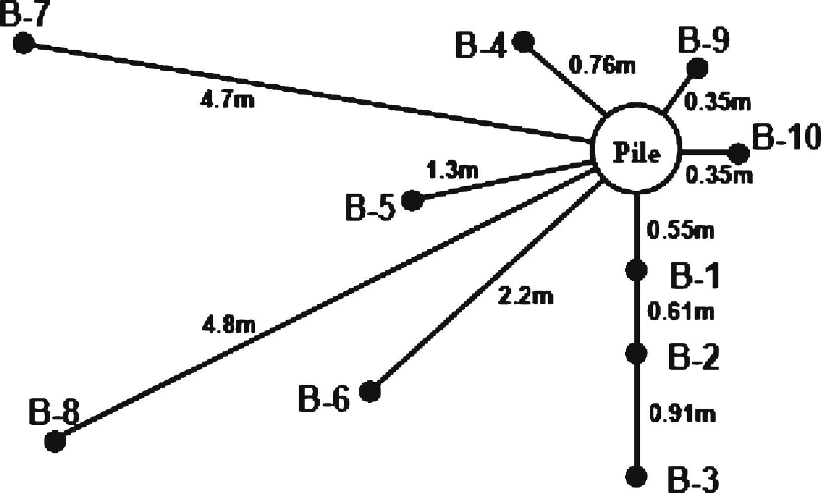
Fig.2
Map of YBM site locations used in the calibration of the MIT-S1 model. Source: Google maps.
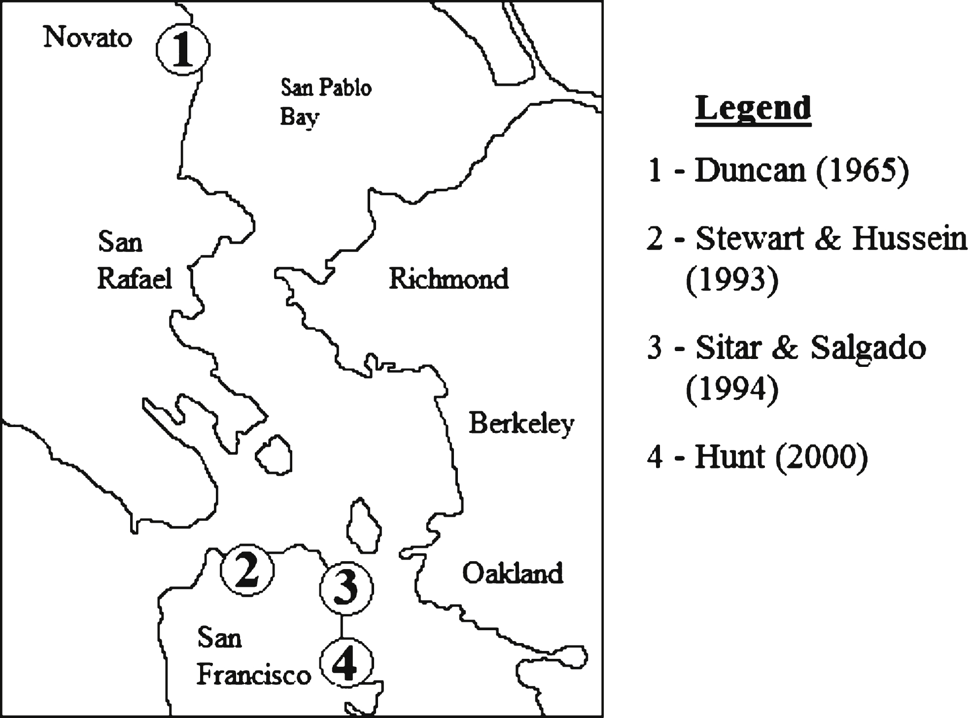
Fig.3
Determination of parameters ρc, D, r and h from measured 1-D loading and unloading in constant rate of strain oedometer tests.
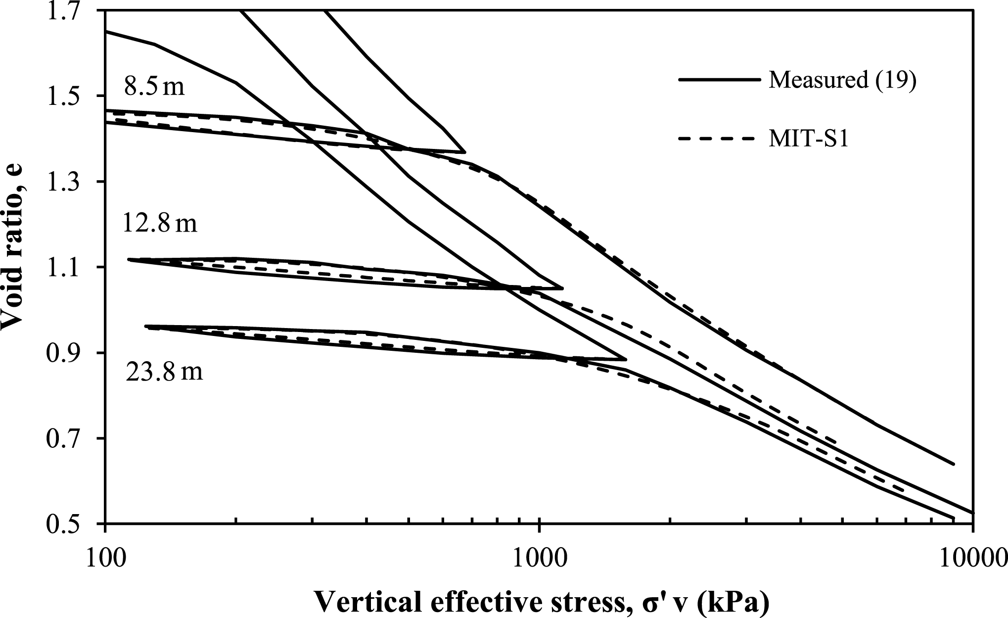
Fig.4
Determination of parameters μ′0 and ω.
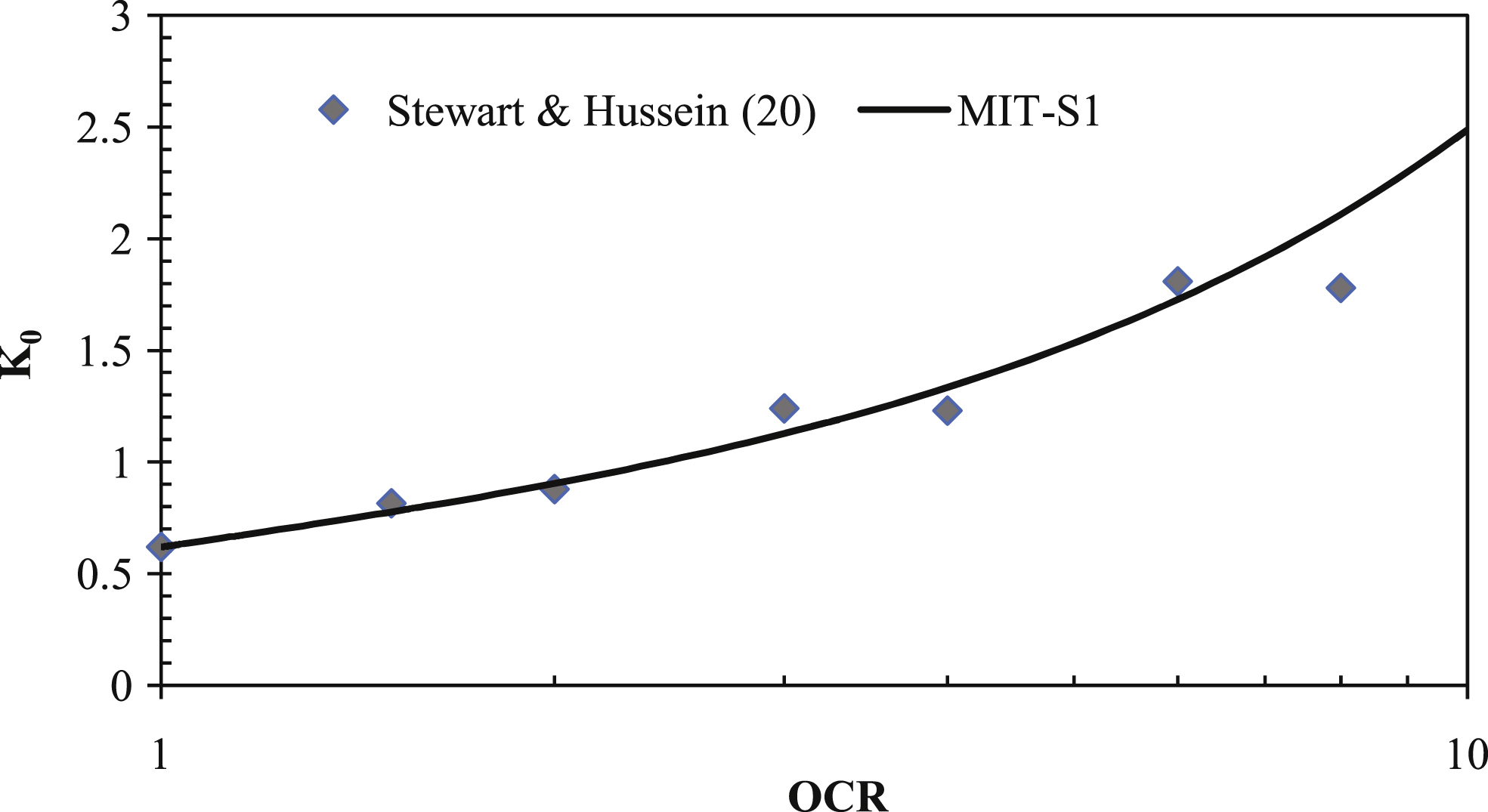
Fig.5
MIT-S1 calibrated predictions vs. measured stress paths in triaxial compression.
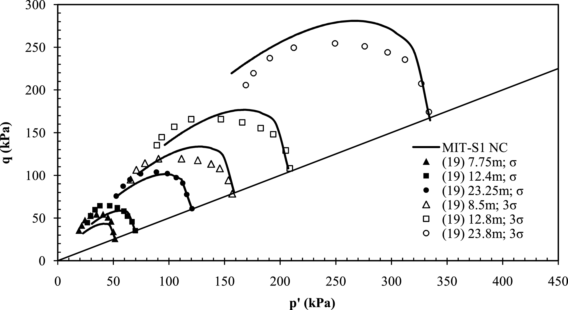
Fig.6
Calibration of ψ to measured stress-strain curves.
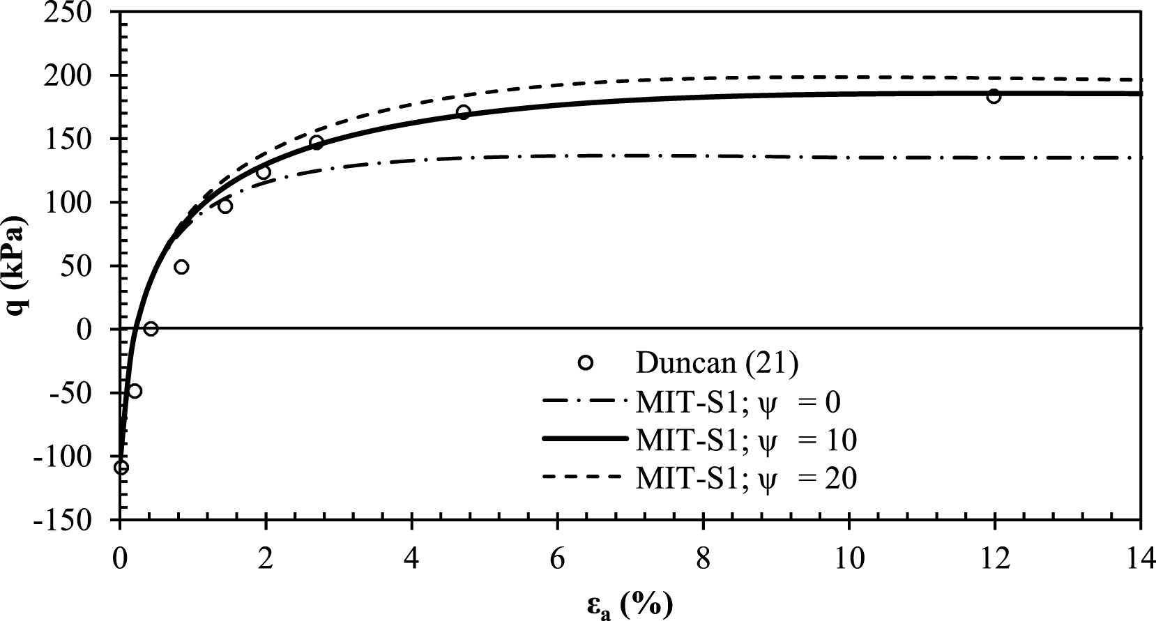
Fig.7
Determination of small strain non-linearity in shear.
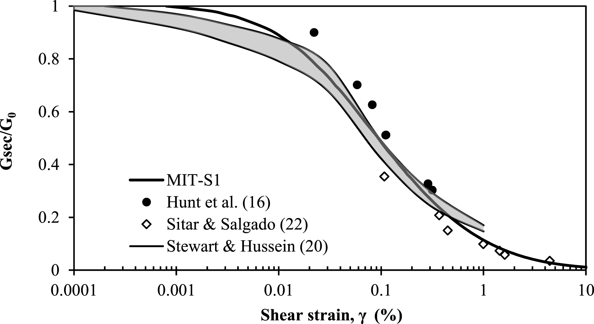
Fig.8
Determination of parameter Cb from data reported in the literature.
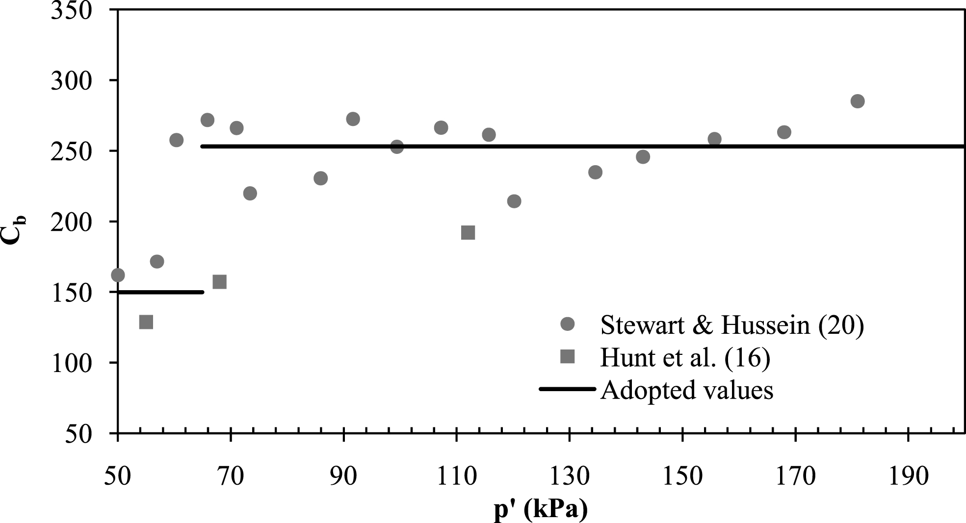
Fig.9
MIT-S1 calibrated predictions vs. measured stress-strain curves in triaxial compression.
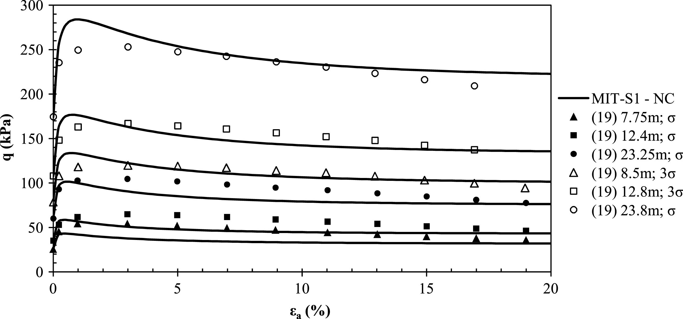
Fig.10
MIT-S1 calibrated predictions vs. measured pore pressures in triaxial compression.
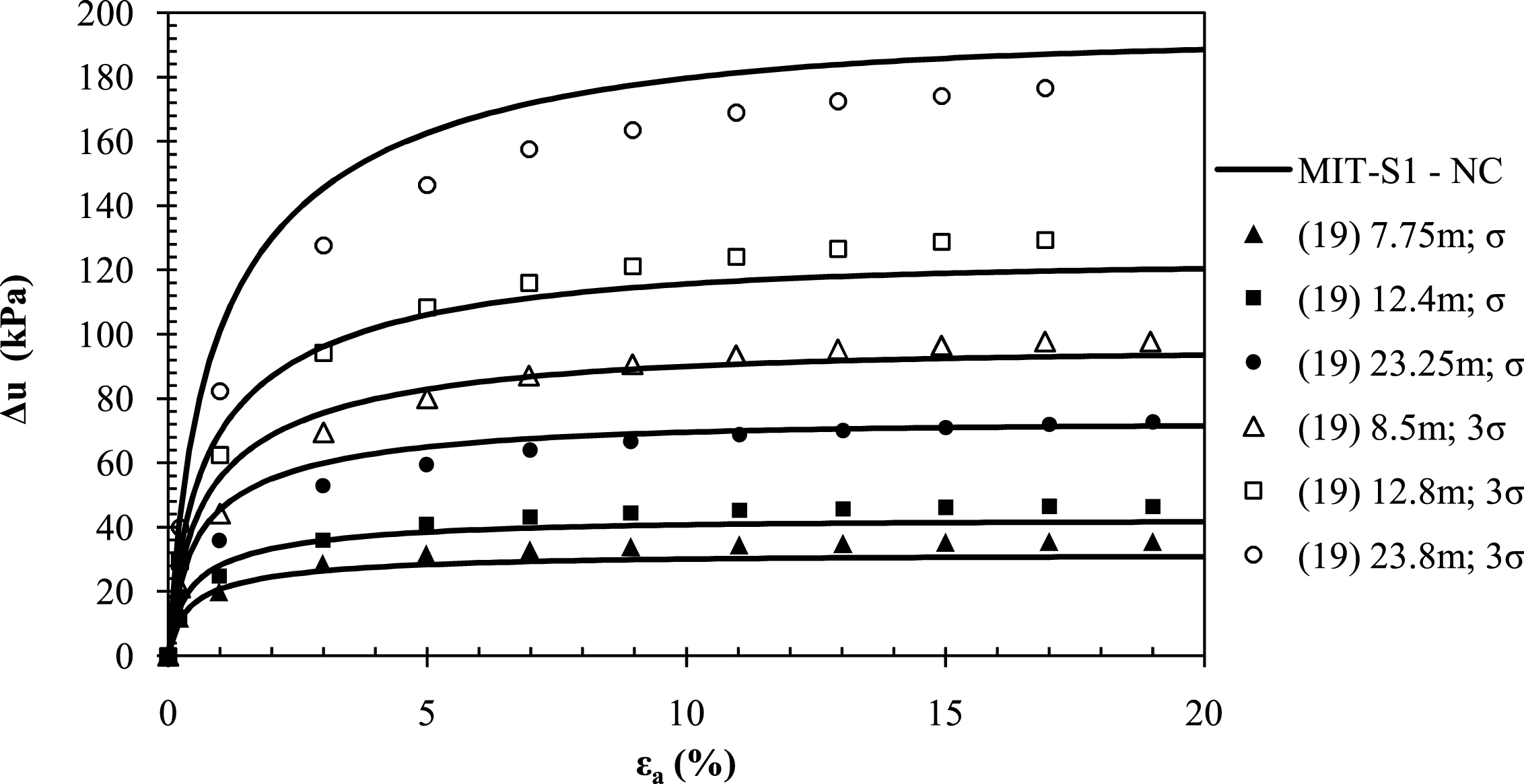
Fig.11
MCC calibrated predictions vs. measured (a) stress paths, (b) stress-strain curves and (c) pore pressures in triaxial compression for 12.4 m depth.
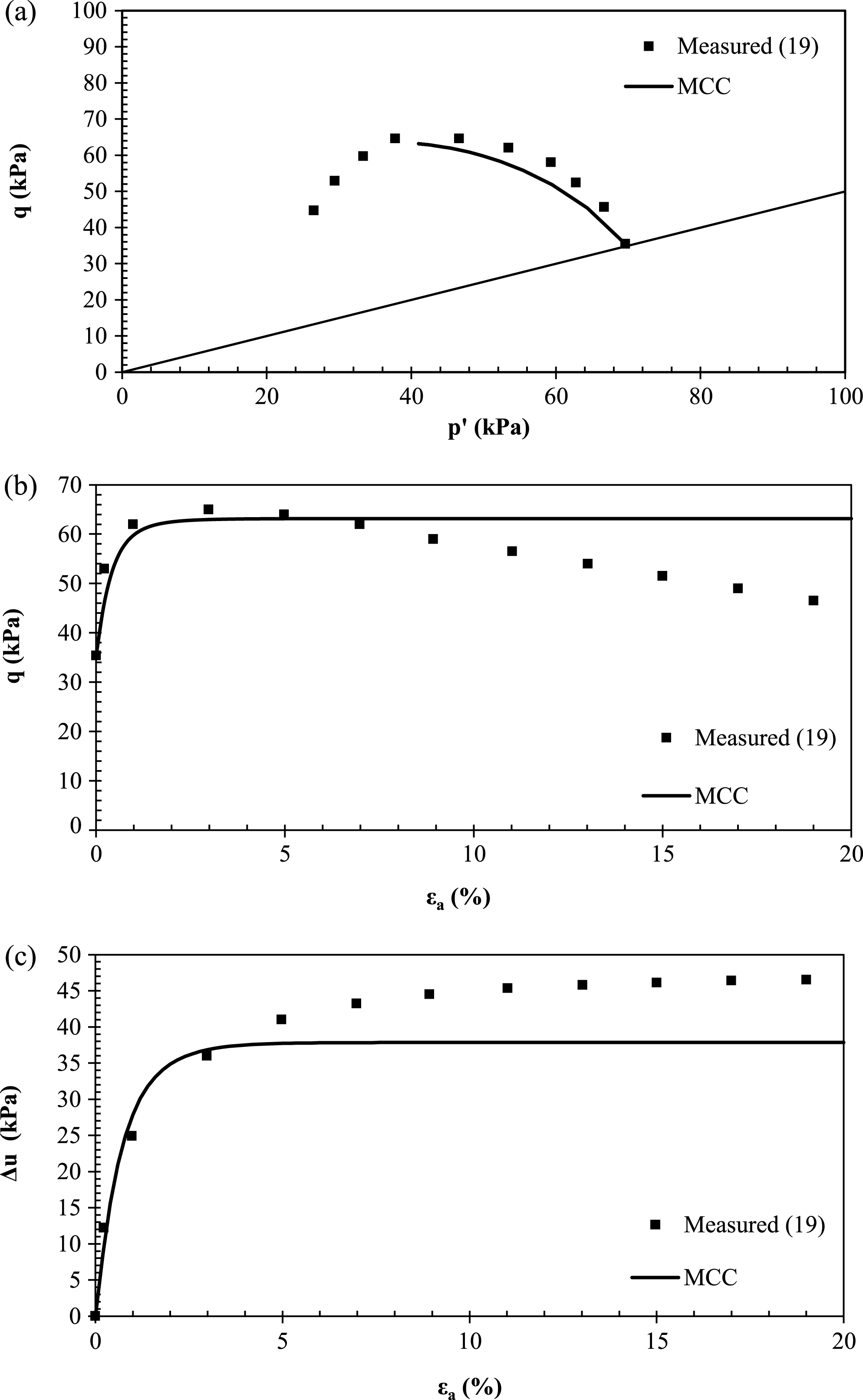
Fig.12
Illustration of prescribed displacements in PLAXIS.
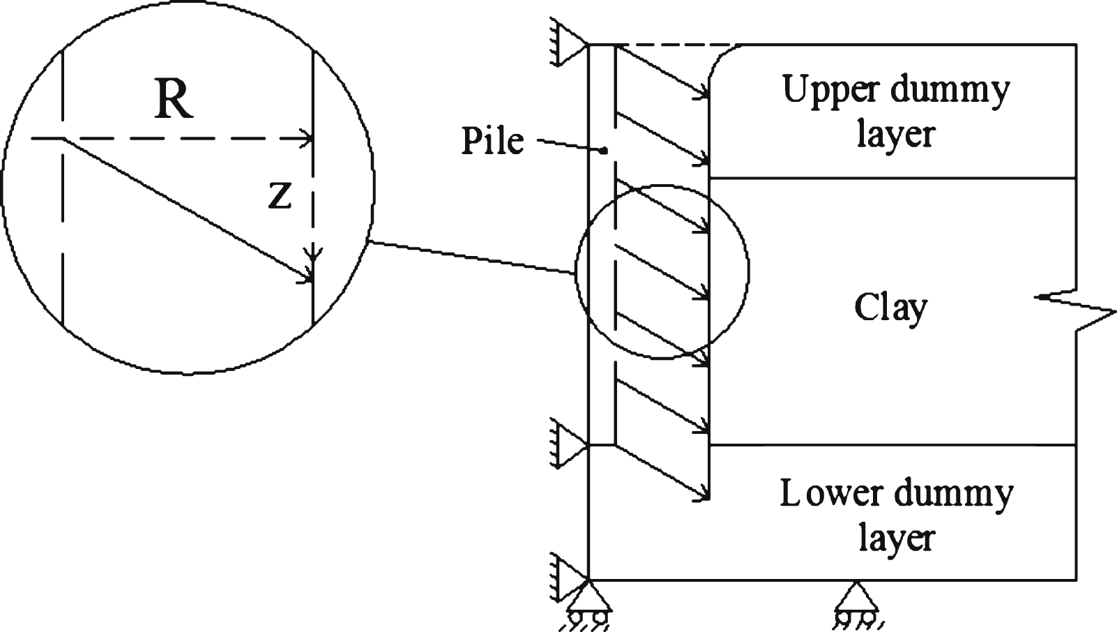
Fig.13
Deformed FE mesh.
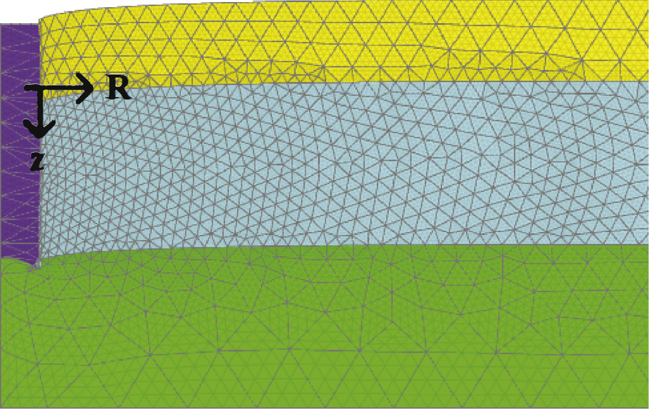
Fig.14
Volumetric tunnel expansion model.
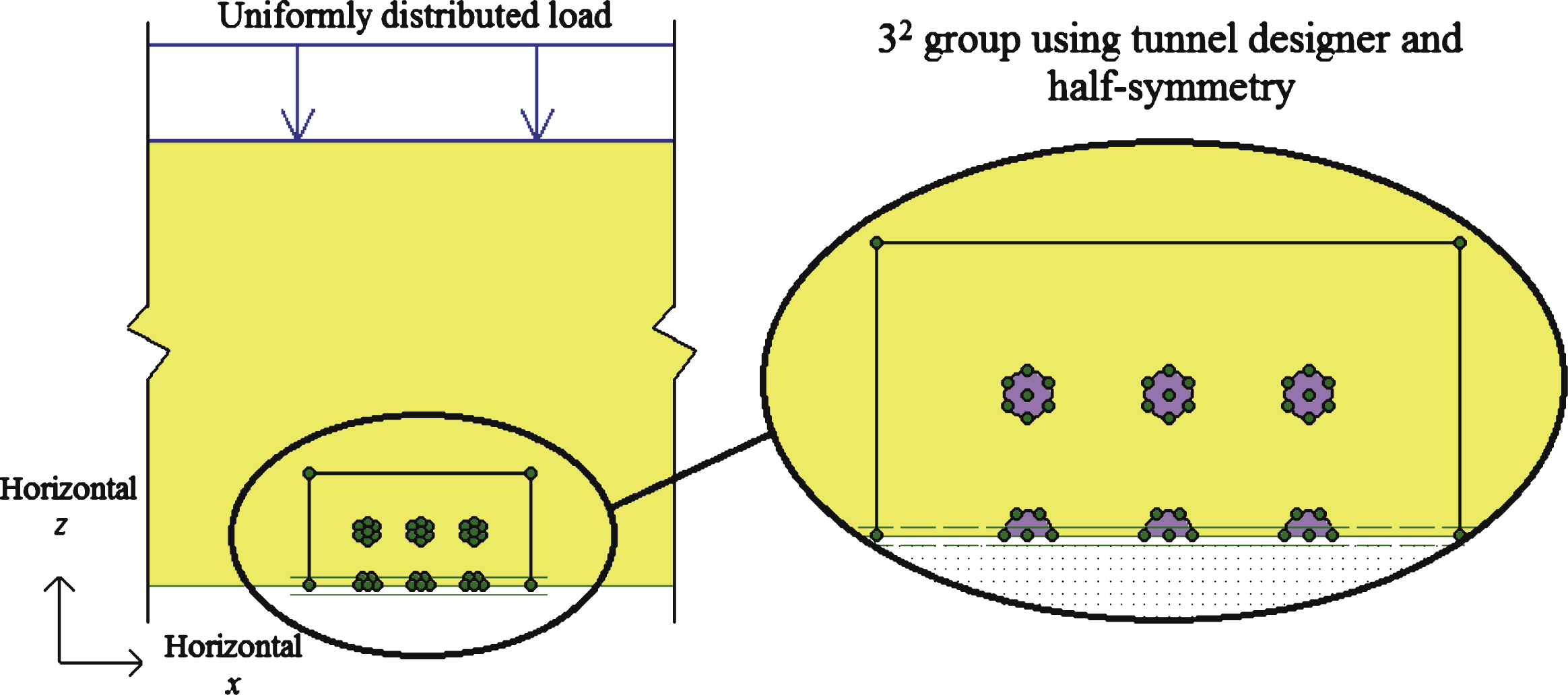
Fig.15
Generated pore pressures at (a) 8.5 m, (b) 12.8 m and (c) 23.8 m depths.
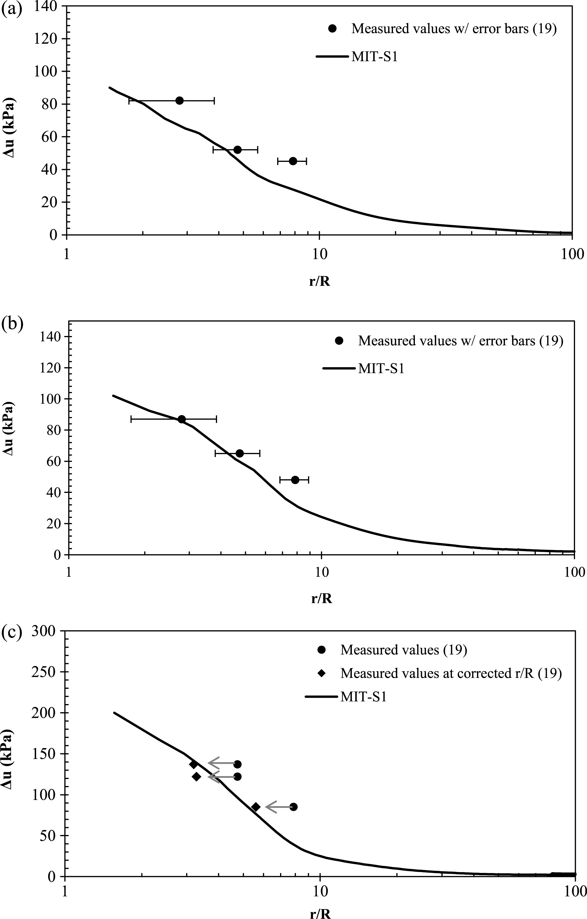
Fig.16
Radial displacements from pile installation and subsequent consolidation.
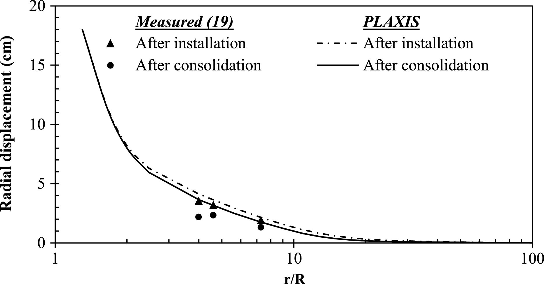
Fig.17
Variations in
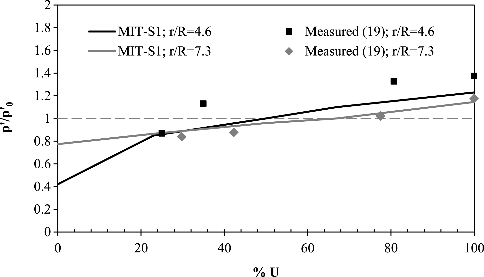
Fig.18
Variations in (a) Δu/σ′v0, (b) σ′rr/σ′rr0 and (c)
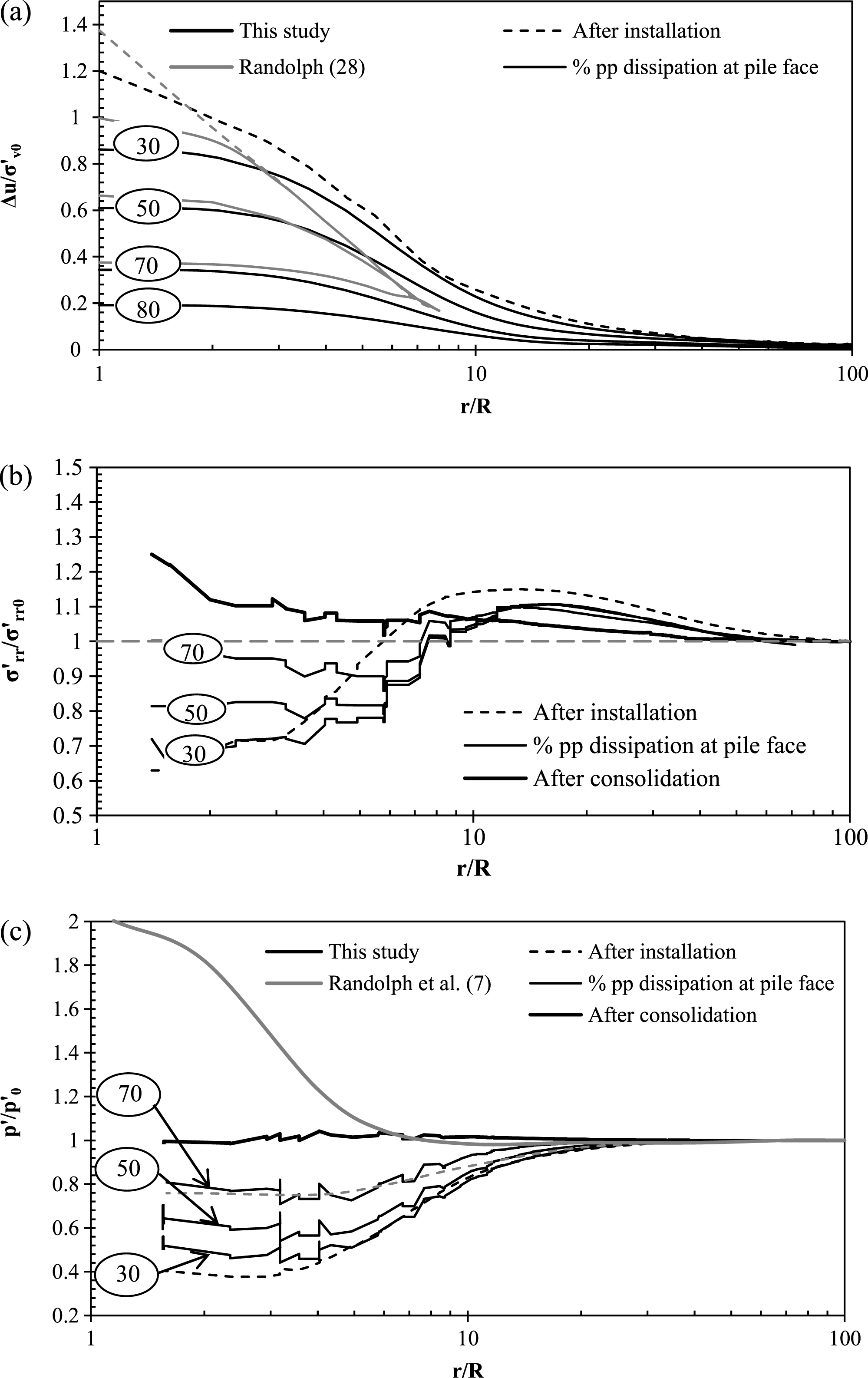
Fig.19
Influence of OCR on lateral distribution of (a) σ′rr/σ′rr0 and (b)
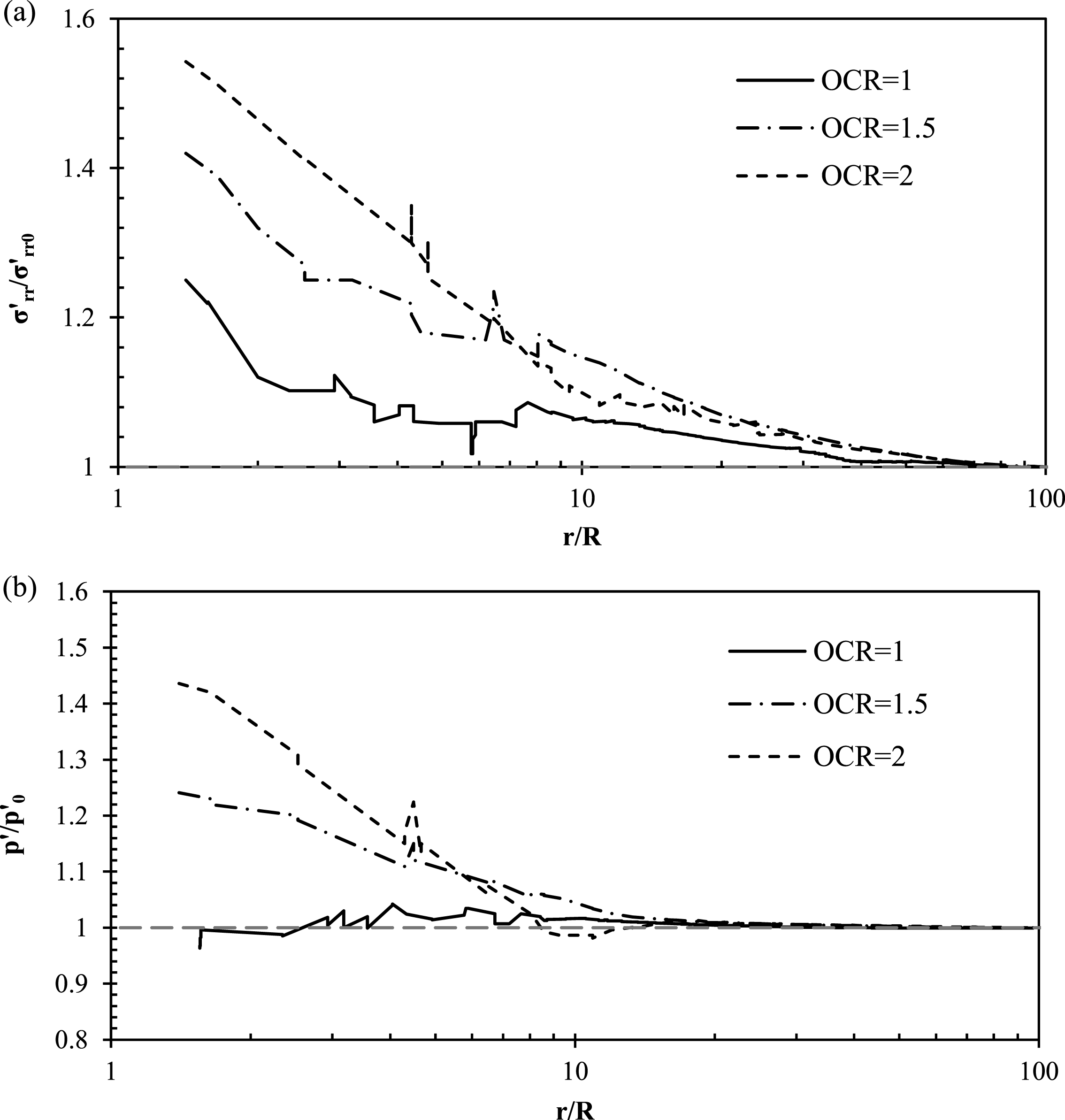
Fig.20
Influence of soil type on lateral distribution of (a) and (b) after consolidation.
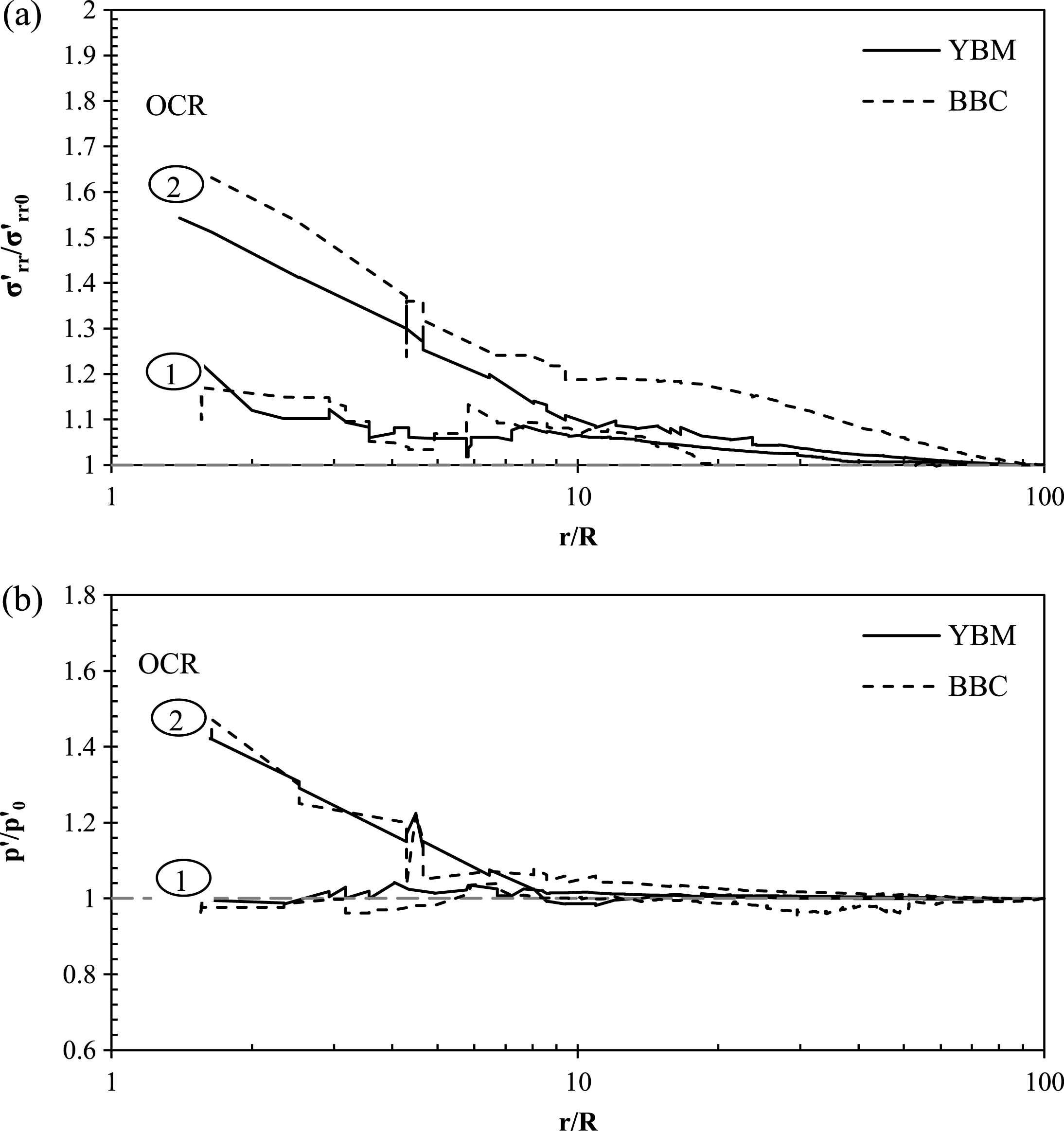
Fig.21
Influence of constitutive model on lateral distribution of p′/p’0 after consolidation.
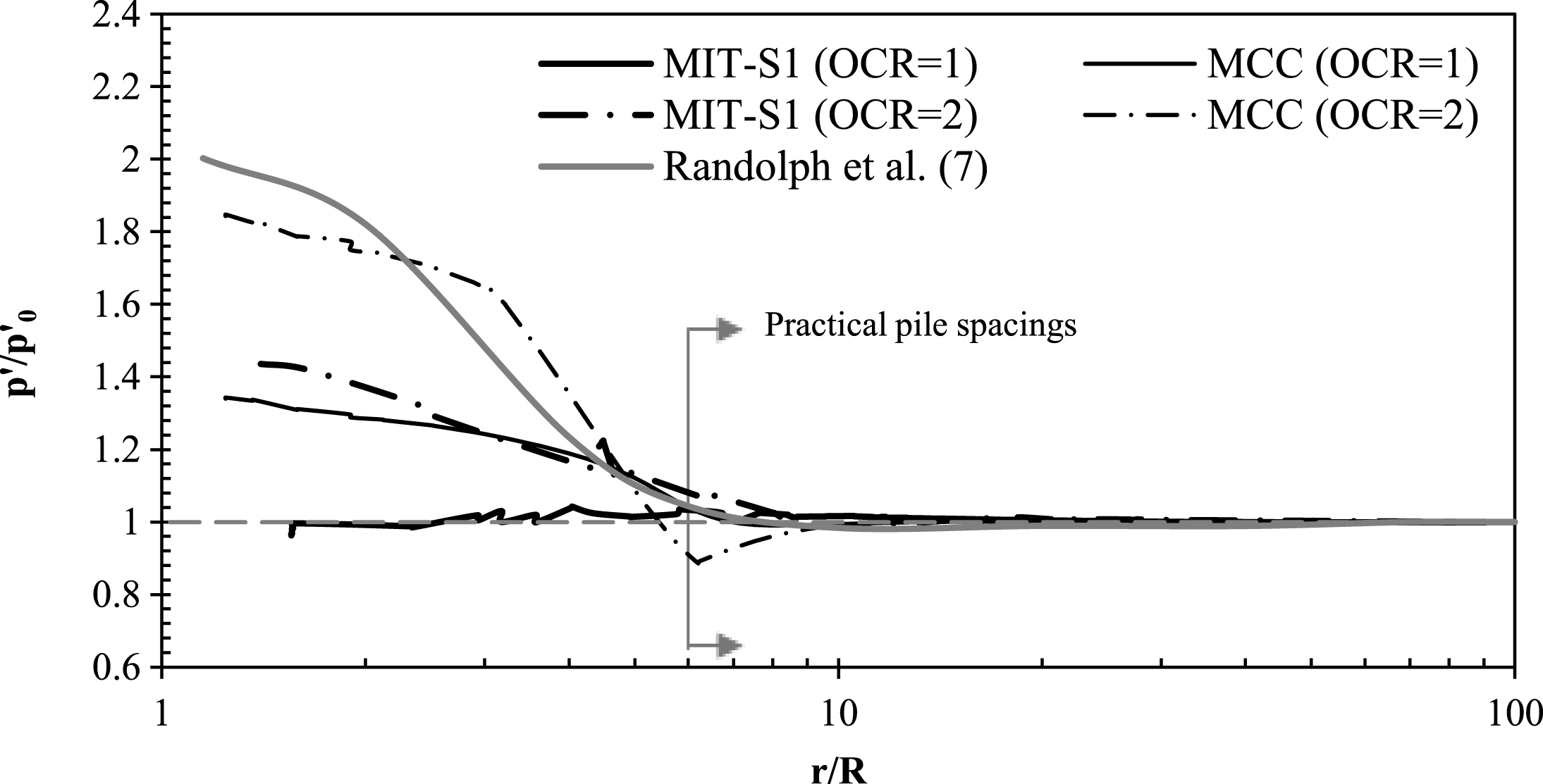
Fig.22
Comparison of (a) Δu/σ′v0 and (b) p′/p’0 predictions around a single pile.
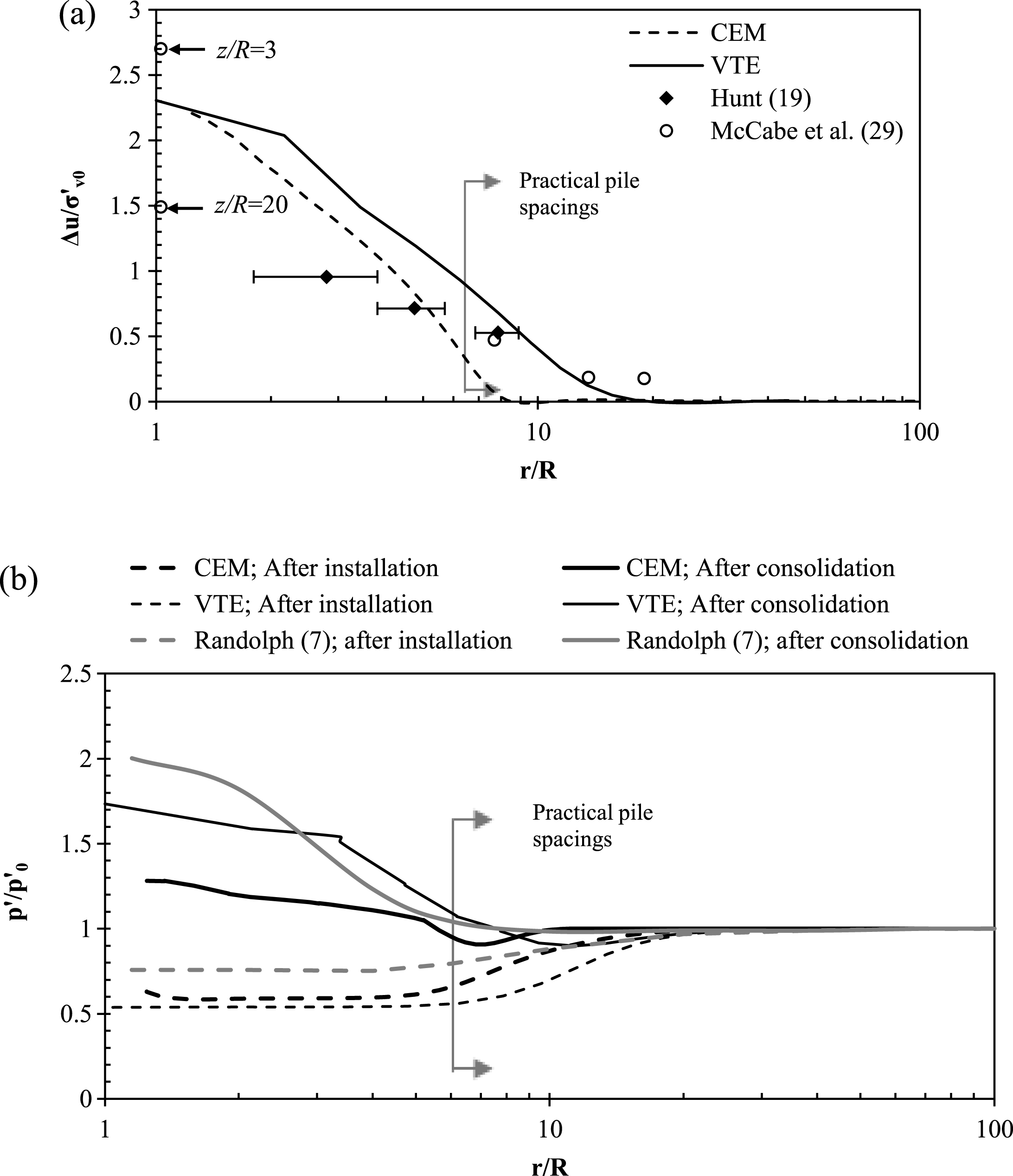
Fig.23
Illustration of pore pressures surrounding 9-pile group after installation; s/D = 3, OCR = 1.
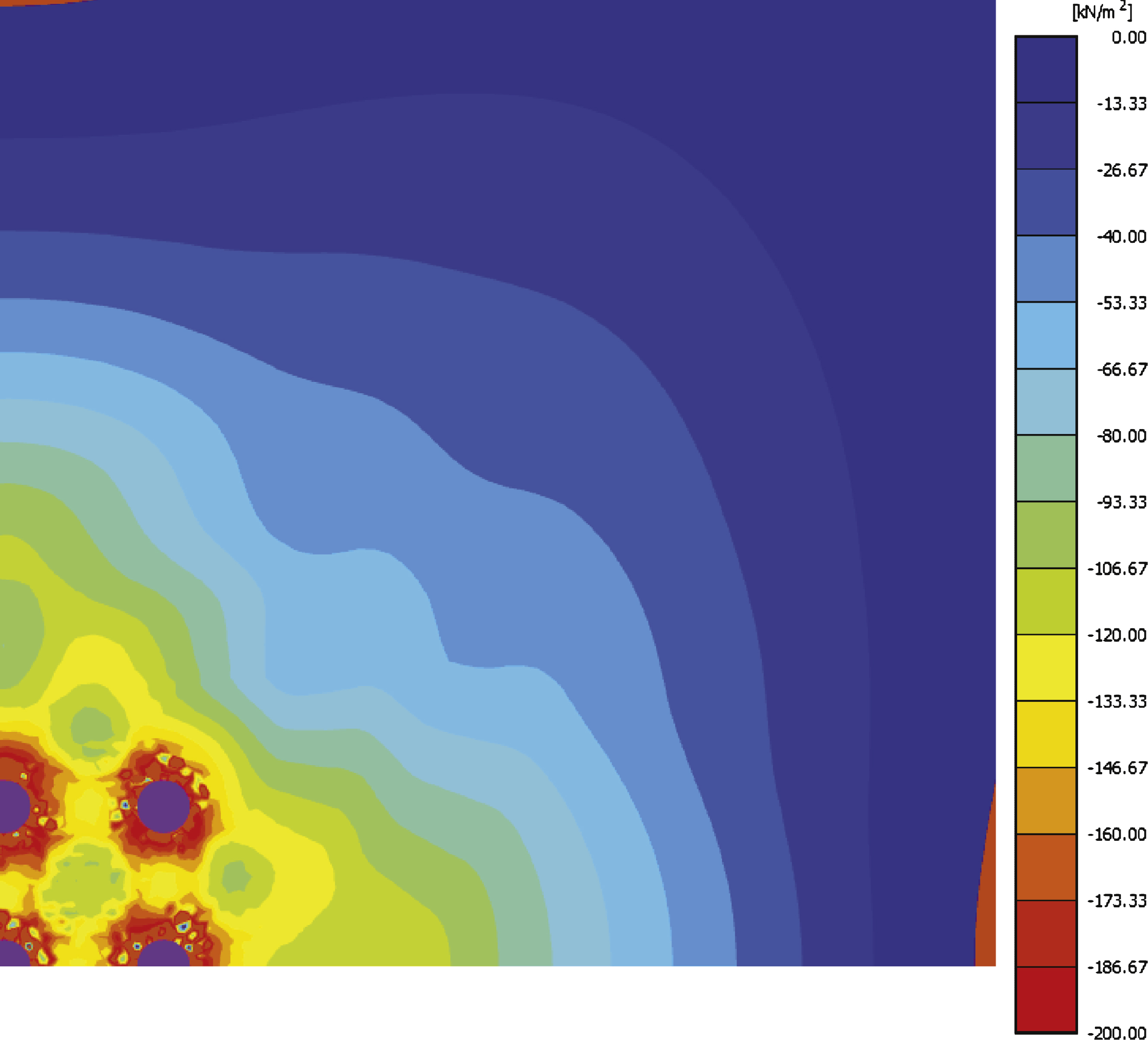
Fig.24
Configuration and cross-section taken of 9-pile group.
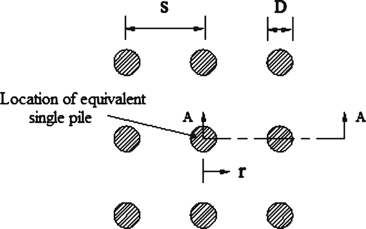
Fig.25
Comparison between single pile and pile group pore pressure distributions after installation; s/D = 3, OCR = 1.
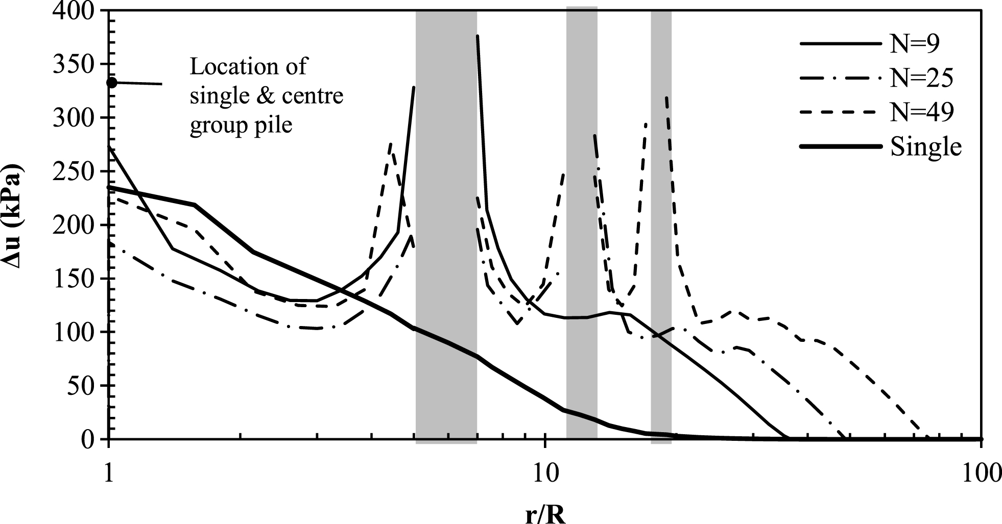
Fig.26
Influence of group effects on (a) ΔuG/ΔuS and (b) p′G/p’S after installation; s/D = 3, OCR = 1.
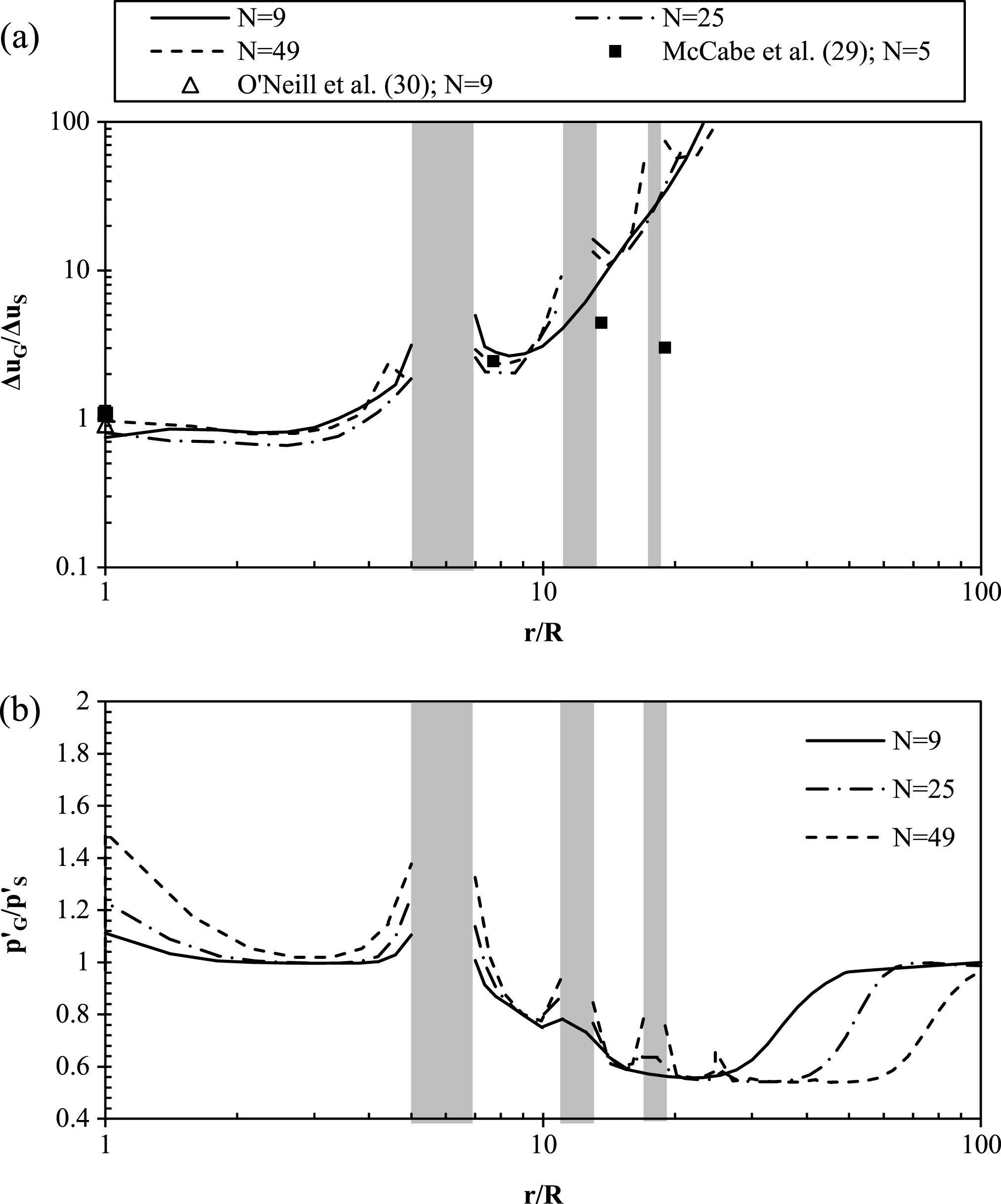
Fig.27
Influence of (a) N, (b) s/D and (c) OCR on p′G/p’S after consolidation; N = 9, s/D = 3, OCR = 1.
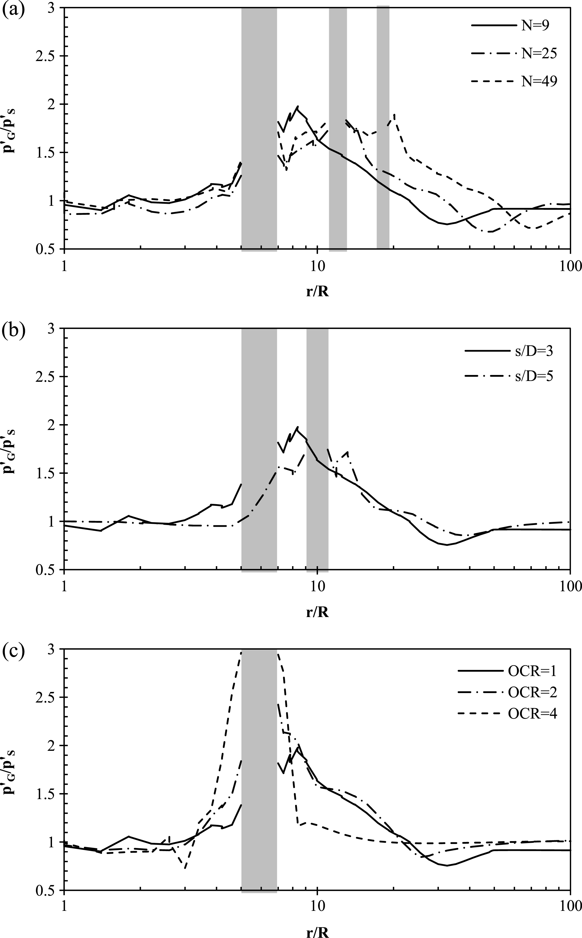
Table 1
Typical index properties of the San Francisco Young Bay Mud at Islais Creek
| Depth (m) | Index properties (%) | Specific gravity Gs | Organic content (%) * | Clay fraction (% <2μm) | Coarse fraction (% >74μm) | Average w (%) | Average γt (kN/m3) | ||
| LL | PL | PI | |||||||
| 8.5 | 98 | 39 | 59 | 2.75 | 4.5 | 50 | 1.5 | 92.2 | 14.3 |
| 12.8 | 86 | 34 | 52 | 2.71 | 4.5 | 45 | 1.7 | 79.8 | 15.1 |
| 23.8 | 76 | 32 | 44 | 2.66 | 4.5 | 48 | 0.6 | 63.4 | 16.2 |
Table 2
MIT-S1 parameters for San Francisco YBM
| Parameter | Physical meaning | YBM | BBC | ||
| 8.5 m | 12.8 m | 23.8 m | |||
| ρ c | Compressibility of normally consolidated (NC) clay | 0.275 | 0.283 | 0.268 | 0.178 |
| D | Nonlinear volumetric swelling behaviour | 0.03 | 0.03 | 0.03 | 0.04 |
| r | 0.8 | 0.8 | 0.8 | 0.85 | |
| h | Irrecoverable plastic strains | 10 | 10 | 10 | 6 |
| K0,NC | K0 for NC clay | 0.62 | 0.62 | 0.62 | 0.49 |
| μ′0 | Poisson’s ratio at load reversal | 0.2 | 0.2 | 0.2 | 0.24 |
| ω | Nonlinearity in Poisson’s ratio; 1-D unloading stress path | 2 | 2 | 2 | 1 |
| φ′cs | Critical state friction angle in triaxial compression | 35° | 35° | 35° | 33.5° |
| φ′m | Apex angle of bounding surface | 43 | 43 | 43 | 46° |
| m | Shape of bounding surface | 1.3 | 1.3 | 1.3 | 0.8 |
| ψ | Rate of evolution of anisotropy due to stress history | 10 | 10 | 10 | 15 |
| ω s | Small strain nonlinearity in shear | 6 | 6 | 6 | 8 |
| Cb | Small strain elastic compressibility (at load reversal) | 150 | 250 | 250 | 450 |
| e0 | Initial void ratio | 2.46 | 2.07 | 1.71 | 1.0 |
Table 3
MCC parameters for San Francisco YBM at a depth of 12.8 m at Islais Creek
| Parameter | Physical meaning | |
| λ | Gradient of the virgin isotropic compression line in e-ln p’ space | 0.42 |
| κ | Mean gradient of the swelling and recompression line in e-ln p’ space | 0.044 |
| M | Value of the stress ratio q/p’ at the critical state condition | 1.54 |
| μ ur | Elastic Poisson’s ratio | 0.25 |
| e0 | Initial void ratio | 2.07 |


