
Annual daylight simulations with EvalDRC – Assessing the performance of daylight redirection components
Abstract
EvalDRC is a newly developed daylight analysis tool for the evaluation of Daylight Redirecting Components (DRC) in architectural spaces. It focuses on the accurate simulation of light redirection with help of the lighting software environment RADIANCE. It employs various key technologies, among them are: a) the daylight coefficient method, b) characterisation of the light redirection behaviour of materials and specially designed systems with appropriate data models, and c) daylight metrics. We present several enhancements to these key technologies and the currently existing tools. In the context of daylight coefficients, we improve the solar contribution calculation by using realistic 0.5° solid angle sun primitives, thus generating True Sun coefficients. For simulating light redirection behaviour, we introduce Contribution Photon Mapping, a recent add-on to the RADIANCE environment. In addition, we introduce monthly breakdowns of the established daylight metrics Spatial Daylight Autonomy (sDA) and Annual Sunlight Exposure (ASE), to provide a more detailed assessment of DRC performance throughout the course of a year. The paper gives an overview of the mentioned annual daylight simulation key technologies. It also explains how our enhancements and developments surpass the current approaches and lead to a versatile tool, capable of producing meaningful and detailed simulation results. A description of the implementation and an application example is given, rounded off by a discussion of the current state of the on-going work and a tentative outlook.
1Introduction
Daylight Redirection Components (DRC) as part of Complex Facade or Fenestration Systems (CFS) can play an important role in reducing the amount of energy used for artificial lighting by increasing the daylight levels in the interior space. However, a quantitative analysis of the impact of DRCs on the interior lighting levels is a difficult task. Due to the dynamic nature of daylight, the typical static illuminance calculations used in artificial lighting design only provide little information about the performance in the annual average. Additionally, DRCs exhibit complex light reflection, transmission, redirection and scattering characteristics, which demand elaborate techniques for producing reliable simulation results. Mathematical models for the generation of sky radiance distributions based on local weather data are needed to provide a representative input for the general amount of available daylight at a specific location. The lighting simulation step finally has to be followed by suitable data reduction mechanisms, to convert large annual data sets into some meaningful figures describing the useful interior daylight availability.
Dynamic Daylight Simulations (DDS) have been a topic for on-going research for a long time. In recent years, much progress has been made in this field by the introduction of various key technologies. The daylight coefficient method provides an efficient strategy for handling annual simulation runs (Bourgeois, Reinhart, & Ward, 2008). Light redirection characteristics of DRCs can be simulated with measured data of the bidirectional scattering distribution function (BSDF) (Ward, Mistrick, Lee, McNeil, & Jonsson, 2011). Both mentioned technologies are implemented within the RADIANCE 3 Phase Method (McNeil, Lee, 2013) and the DAYSIM (Reinhart, 2000, DAYSIM) program suite, which, to a certain extent, constitute the current standard for annual daylight simulations. Finally, suitable daylight metrics have been developed, which reduce annual simulation data to a small set of indicators. An example of a commonly established metric is the combination of Spatial Daylight Autonomy (sDA) and Annual Sunlight Exposure (ASE), proposed by the Illuminating Engineering Society of North America (IESNA) (Heschong et al., 2012).
However, the mentioned key technologies and their implementation in the currently established simulation tools do not perform equally well in all conceivable scenarios. While the actual methods for the daylight coefficient calculation adequately represent the light from the sky hemisphere, they are less accurate for the sun contribution. DRCs are designed to respond to precise sunlight positions, thus requiring an accurate treatment of the sun contribution for producing reliable simulation results. In the context of DRC simulation, BSDF data sets are not equally appropriate for all available DRC system types, both in terms of their measurement and their use in simulation tools. Especially distributed DRCs, such as light pipes and ducts, call for other, more appropriate simulation methods. Finally, the daylight metrics sDA and ASE respectively produce a very strong data reduction to an annual scalar value. This allows a quick comparison of different installations with respect to their annual daylight performance, but does not provide information about the DRC performance in different periods of the year. As the sun path over the sky hemisphere shows a strong seasonal variation in all regions except the equatorial zone, DRC response can be expected to follow this variation, which in turn makes it interesting to reflect this in the daylight metrics.
To address the limitations described above, our simulation tool EvalDRC introduces new concepts and enhancements in selected steps of the annual simulation process, while still building on the mentioned key technologies in a general sense. In the daylight coefficient calculation, a particular emphasis lies in the exact treatment of the solar contribution. Additional to the BSDF strategy, light redirection characteristics of DRCs are evaluated with Photon Mapping (Schregle, Bauer, Grobe, & Wittkopf, 2015). In contrast to classic backward ray tracing algorithms, Photon Mapping or forward ray tracing is capable of simulating the light transport through refracting and reflecting media to a high degree of accuracy. Finally, enhanced versions of existing sDA and ASE daylight metrics at a monthly resolution are proposed. A more detailed metric dataset can be very helpful in identifying critical phases and optimization potential during DRC analysis and development.
2Strategies for daylight simulations
2.1The daylight coefficient method for annual simulations
Annual daylight simulations demand a high number of individual calculations with varying input values due to the dynamically changing sky conditions. In order to handle this task, the daylight coefficient method splits it into two steps. The first step, the coefficient generation, performs the complex light path simulation from the daylight sources (sky and sun) through daylight openings and DRCs and finally via interreflections within the interior space. The second step, the result accumulation, then produces illuminance results for all timestamps of a chosen evaluation period. This is done by adding up the coefficients, weighted with radiance values for the corresponding daylight sources, which are determined from weather data files via mathematical sky models. Of course, the different natures of the two daylight sources, sky hemisphere and sun, demand different strategies for the coefficient generation.
2.1.1Sky coefficients
For the sky coefficient generation, a discrete representation of the sky hemisphere is used, based on the scheme originally proposed by Tregenza (Tregenza, 1987). The hemisphere above the horizon is divided into 145 segments or patches, and one additional hemispherical segment represents the ground reflection. The average solid angle of the segments reflects the aperture angle of 11°, which was a typical value for sky luminance scanners at that time. Using a normalized sky hemisphere as input, the lighting simulation calculation with the RADIANCE rcontrib program then produces a separate record for the partial scene illumination produced by each patch. Dependent on the chosen output format, such a coefficient can either be a single unitless value or an HDR rendering of the scene, illuminated by one specific sky patch (Fig. 1).
2.1.2Solar coefficients
As a moving light source with narrow emission angle (0.5°), the sun initially does not fit into the sky patch discretization concept. To overcome this problem, various ideas have been proposed so far. In the RADIANCE 3 Phase Method, the solar radiance is added to the three neighbouring sky patches which are closest to the current sun position, thereby distributing it over an unrealistically large solid angle. As the average solid angle of the sky patches in the Tregenza scheme is quite high, often a subdivision of the Tregenza patches by small powers of 2 is applied. This avoids distributing the solar radiance over unrealistically high solid angles (Fig. 2, left). The DAYSIM tool uses a different approach. Separate solar contributions are calculated for a set of predefined sun positions (currently 65, at approximately 10° angular separation in azimuth and altitude). Then each actual solar contribution can be determined by averaging the results from four neighbouring predefined positions. (Fig. 2, second from left).
As the sun contribution to interior illumination is generally much higher than that of the sky hemisphere, both methods suffer from the disadvantage that the most valuable contribution is treated in the least accurate way. This becomes even more important when redirection of sunlight by DRCs comes into play. For systems with sharp peaks in the redirection characteristic, the distributed or averaged input will likely produce inaccurate results if the distribution solid angle exceeds the halved peak width (w.r.t. the incoming direction). One approach of addressing this problem is to increase the sky patch or predefined sun position resolution. This is applied in the RADIANCE 5 phase method (McNeil, 2013), where an additional high-resolution sky patch subdivision with Reinhart factor of 6 is used with patch-centred predefined suns in a separate step for adding the solar contribution (Fig. 2, second from right).
2.1.3True sun coefficients
In the new EvalDRC tool, the original Tregenza subdivision into 145 patches is used for the sky, while the solar radiance is not distributed or averaged at all. Separate coefficients are calculated by using exact 0.5° angular sun source primitives for all timestamps of the evaluation period (Fig. 2, right). Therefore, we introduce the term True Sun Coefficient, to distinguish them from the approximated solar coefficients described above. In theory, this provides the maximum possible accuracy for the treatment of the solar contribution. However, it demands a considerably increased calculation effort compared to the aforementioned more abstract methods (with exception of the RADIANCE 5 Phase Method, with its high predefined sun position count).
2.1.4Coefficient accumulation: From coefficients to contributions
The coefficients are only intermediate results. They can be understood as potential contributions, indicating how much a source might contribute to the scene illumination. To generate a final HDR rendering of a scene or illuminance values on a sensor plane, one needs to perform a weighted superposition of all coefficients, using the radiances of the sky patches and the solar radiance as weight factors. For daylight sources, the coefficients or potential contributions can be assumed to initially scale with the solid angle of emission (cf. Table 1).
Of course, the scene geometry and material properties then determine the quantity and extent of light from these different emission directions reaching the interior scene and how it is further distributed throughout it. Based on this information, the radiances used as weighting factors finally determine how much a source (or a source patch) actually contributes to the lighting. Thus a high coefficient does not automatically imply a high contribution. In contrast, the high solar radiance (compared to sky and ground reflection) generally outweighs the smaller coefficient size by far, making the solar contribution the substantially dominant component.
One set of coefficients suffices to generate results for several different timestamps by simply applying the corresponding time dependent radiance distributions for each of them in the superposition step. This is a key aspect of the coefficient method, and explains why it is very efficient for annual daylight simulations, which otherwise would need a lot of individual simulation runs. Evidently, our approach using exact sun positions in the coefficient calculation partly breaks this flexibility with respect to the solar part. The True Sun Coefficients are fixed to the timestamps they are generated for.
2.2Methods for the simulation of light redirection methods
Algorithms for general lighting simulation are established and validated already for some decades. The most common strategies are the radiosity and the ray tracing method. The simulation of DRCs however poses additional challenges to the simulation algorithms beyond those of general lighting simulations. DRCs come in a wide variety of geometric shapes and material combinations (Fig. 3), but they commonly deflect the light from its straight path upon passing through the system. Only the ray tracing method is generally capable of simulating such complex light redirection behaviour; traditional radiosity only accounts for diffuse light transfer. Two ray tracing based strategies have proven themselves a valuable means for this task, notably a) using ray tracing algorithms capable of evaluating BSDF data and b) the Photon Mapping technique.
2.2.1BSDF data
The BSDF, or bidirectional scattering distribution function, is a means of describing light redirection from incoming into outgoing directions for a specific point on a surface. Consequently, BSDF data are dimensionless values, representing the ratio of emitted radiance to incoming irradiance (Richmond, Hsia, Ginsberg, & Limperis, 1977). The whole set is often separated into two different components BRDF and BTDF for reflection and transmission. For DRC simulations, usually only the transmission is of interest, so we limit our description to this component here. The functional representation in theory describes the light redirection in an infinitesimal resolution. In practice, often a finite data set is used instead (Fig. 4). Both incoming and outgoing hemispheres are subdivided into sections, and the BSDF data constitute a tabular representation of the BSDF values for all incoming and outgoing section combinations.
BSDF data can be measured with goniophotometers (GPs) or calculated e.g. with forward ray tracing programs (Grobe, Noback, Wittkopf, & Kazanasmaz, 2015; McNeil, Jonsson, Applefield, Ward, & Lee, 2013). Depending on the material and/or geometric properties, a large amount of data might be necessary to adequately describe the redirection characteristics of the system or material (Fig. 5). With scanning GPs, measurements can be performed with significantly higher resolution, but the process is more time consuming, compared to image based GPs (Krehel, Kämpf, & Wittkopf, 2015; Apian-Bennewitz, 2010). To a certain extent, the characterisation of a DRC with a BSDF data set can be seen in analogy to the description of artificial luminaires with lighting intensity distribution data (LDCs).
Evidently, the use of BSDF data increases the level of abstraction in the simulation process. The finite resolution of the data set may introduce accuracy problems, if the section or patch size (cf. Fig. 4) does not suit the complexity of the redirection characteristic. Simply raising the angular resolution leads to an increase of the data amount by a power of two, producing data files which claim a large portion of system memory during the simulation run. However, for the majority of systems and materials, a high angular BSDF resolution is only needed for selected solid angle regions, so variable resolution data storage formats have been developed, e.g. the so-called Tensor Tree BSDF (Ward, Kurt, & Bonneel, 2012).
RADIANCE fully supports the use of BSDF data since version 4.2. The RADIANCE 3 Phase Method relies on the use of BSDF data representations for DRCs to perform annual daylight simulations. EvalDRC also builds upon the RADIANCE BSDF support as one of two general methods provided for light redirection simulation (cf. Sect. 2.2.2).
2.2.2Contribution photon mapping
Photon Mapping, originally introduced by Wann Jensen (Wann Jensen, 2001), is a variant of the general ray-tracing algorithm in which rays (photons) are emitted from the light sources. This is in contrast to the classic backward ray tracing, where rays are initially emitted from the view point. The forward path tracing constitutes the ability to accurately simulate the light particle transport through complex refracting and reflecting media, which is – cum grano salis – principally impossible to achieve with the normal backward ray tracing method. Therefore, Photon Mapping is an interesting technique for DRC simulations. A first Photon Map module for RADIANCE was developed and validated in 2002 (Schregle, 2004). Recently, this Photon Map module was enhanced to include support for the contribution coefficient method (cf. Sect. 4) and finally was integrated into the main RADIANCE distribution.
The new Contribution Photon Mapping (Schregle, 2015; Schregle, Grobe, & Wittkopf, 2015) offers the possibility to sort the individual light source contributions into different bins during the final gathering. By introducing the concept of primary photons (Fig. 6), which carry the information about the emitting light source, additionally a dynamic binning dependent on the emission direction is possible. This connection to its original light source and emitting direction is of course necessary to use Photon Mapping in the daylight coefficient method (cf. Sect. 2.1). Coefficient calculation was impossible with the previous Photon Map version, because the photons were unaware of their origin.
2.3Data reduction with daylight metrics
Daylight metrics (DM) are special criteria for quantifying the useful daylight availability in interior spaces. They are generated from large sets of lighting simulation results with different reduction techniques with respect to space and time. Ideally, not only the amount of daylight, but also discomfort problems due to glare should be considered in the evaluation algorithm. This demands annual simulations, which reflect the current building and room scenario to a sufficient degree of realism, both statically (room geometry, furniture, material properties) and dynamically (location specific weather data, dynamic sunshade operation). Evidently, in practice various abstractions might be introduced when exact data are either not available or too complicated to be considered in the simulation.
DMs can be seen as successor to the former daylight factor, which they surpass by far in terms of information content. The daylight factor has more in common with the coefficients (cf. Sect. 2.1), because it is a dimensionless ratio of interior to exterior daylight illumination, being further limited to overcast sky conditions only.
Among the several DMs which have emerged, the Spatial Daylight Autonomy (sDA) and the Annual Sunlight Exposure (ASE) as defined by the IESNA have received a widespread acceptance, and thus were chosen for integration into EvalDRC. For both metrics, a defined evaluation period of one year is assumed, consisting out of five-day working weeks with occupancy hours from 8 a.m. to 6 p.m. Simulation results and weather data used for generating the sky radiance distributions should be provided at an hourly resolution. The scene should be modelled according to its actual use case, so e.g. office rooms also should include basic models of the furniture. The metric calculation itself is based on illuminance values on a sensor point grid as input, with defined limits for maximum grid point spacing. For a detailed description of all requirements, definitions and discussions about justification of the chosen strategies and thresholds, see Heschong et al. (2012).
2.3.1Spatial daylight autonomy (sDA)
This metric describes the amount of available and useful daylight for a given sensor plane. It is defined as: “the percent of an analysis area [...] that meets a minimum daylight illuminance level for a specified fraction of the operating hours per year” (Heschong et al., 2012).
The sDA calculation is performed in a two-step process. The first step occurs in the time domain. All grid points are recorded which exceed a given illuminance threshold for a given fraction of the total evaluation time. The second step is then executed in the spatial domain. The resulting sDA value represents the fraction of the sensor plane area, which fulfils the criterion of receiving the specified amount of daylight illumination for the given fraction of the total occupancy time. The recommended default settings are 300 lux for the illuminance threshold and 50% for the temporal fraction threshold. Final sDA values above 55% are categorized as nominally acceptable, values above 75% as preferred daylight availability.
With the default thresholds one takes into account that daylight will not be available to a sufficient extent throughout the whole year. But the thresholds may be adjusted individually. Dependent on the tasks performed in the room, a higher or lower illuminance threshold might be reasonable, and dependent on different occupancy scenarios a higher or lower temporal fraction for attaining and exceeding the illuminance threshold might be justified. In order to distinguish sDA metrics with different thresholds, these are appended as subscripts. The default sDA is thus correctly written as sDA300,50%
When we assume a grid of N points, and define a function S(j), which is 1 for each grid point j which receives a sufficient illuminance for more than the given fraction of total occupancy time, else 0, the sDA can be expressed as:
(1)
where
In the simulation, sun shading has to be considered for – at least – those timestamps, in which direct sunlight illumination on the sensor plane exceeds a specified amount. Calculating these threshold levels for sunshade operation is closely related to the second part of the metric, the ASE value (cf. Sect. 2.3.2). The consideration of sun shading finally justifies the sDA’s meaning as indicator for the amount of useful available daylight.
2.3.2Annual sunlight exposure (ASE)
The aim of this metric is to quantify both glare problems and possible solar gains. It is defined as: “the percent of an analysis area [...] that exceeds a specified direct sunlight illuminance level more than a specified number of hours per year” (Heschong et al., 2012).
The interesting aspect is that, again, grid point illuminance data are used as basis. So no further simulations, such as field of view renderings for identification of regions with disturbingly high luminances, are needed. However, unlike the sDA case, the illuminances calculated for the ASE metrics must only include the contribution from direct sunlight or purely specular sunlight reflections. For lighting simulations with RADIANCE, this simply means to disable the indirect calculation by setting the ambient bounces parameter to zero.
Like the sDA, the ASE metric also operates with illuminance and temporal threshold values, and finally results in a fractional value w.r.t area. With the default settings, grid points which receive at least 1000 lux for more than 250 hours of the annual occupancy time (default thresholds) are recorded, and the fraction of points, or the fraction of the sensor plane area, which fulfils these criteria, determines the ASE value. The thresholds are again added as subscripts, so the default ASE is correctly denoted as ASE1000,250. The mathematical representation is similar to Equation 1
(2)
where
The illuminances used for the ASE explicitly have to be calculated without sunshade, thus the ASE acts as indicator for the amount of direct sunlight reaching the evaluation plane and, in consequence, the need for appropriate measures against it (e.g. sunshade operation and glare control). Categorizing ASE value ranges as acceptable or not is more complicated than in the sDA case. Due to the deliberate simulation without sun shading, the grid point illuminances do not represent a ‘final’ state. Evidently, conditions leading to a high ASE value are those which usually trigger sunshade operation, either automatic or manually by the occupants. In fact, this aspect of the ASE calculation is used in the metric to determine the dynamic sunshade operation thresholds needed for the sDA evaluation (cf. Sect. 2.3.1). Per default definition, sunshade operation is assumed for those timestamps during which 2% or more of the grid points exceeds the above-mentioned 1000 lux illuminance threshold. Consequently, the 2% also represents the nominally acceptable ASE value for a ‘complete’ simulation scenario including sunshade operation.
Again, all ASE thresholds may be adjusted to fit the actual circumstances. Compared to the sDA, the ASE definition based on grid point illuminances rather than field of view evaluations, including the chosen default thresholds, are both subject to a more complex justification argumentation as well as a still on-going discussion. The IESNA reference explores this in great detail.
2.3.3Monthly daylight metric values
The sDA and ASE metric both imply a strong data reduction to one annual value each. When used for comparing different DRCs, this can be enough to make a quick decision about which system performs better in total. But no information about the DRC performance throughout the course of the year can be extracted from the metric. As seasonal variation of daylight availability plays a great role in all regions of the world except the equatorial zones, breaking the annual metrics down into monthly values is a first step of adding more detail and useful information to the daylight metrics by still maintaining a reasonable number of values.
The new equivalents to the annual sDA and ASE metrics are denoted msDA for the Monthly Spatial Daylight Autonomy, and MSE for the Monthly Sunlight Exposure. Their calculation proceeds analogously to the annual values, with the only difference that all temporal thresholds now are interpreted relative to the timestamp count of one month. Similarly to Equation 1, the msDA for month m can be expressed as
(3)
with
Because of the different timestamp count for each month, the function S(j) from Equation 1 now becomes S(j,m), i.e. a function of grid point index j and month m. Analogously to the annual case, the MSE can also be expressed by a similar mathematical expression:
(4)
with
It is important to note that, due to the two step evaluation algorithm with illuminance and temporal fraction thresholds, there is no straightforward relationship between the annual metrics and the average of the monthly values. This can be seen if we examine the contribution of one single grid point. Point j contributes to the annual sDA if:
(5)
and it contributes to the msDA for month m if:
(6)
(7)
This would be equal to Equation 6 only if all monthly occurrence counts of illuminance threshold exceeding for this point j are exactly one twelfth of the annual occurrence count of illuminance threshold exceeding, which cannot be expected in general:
(8)
So each grid point may contribute to a selected monthly msDA and not to the annual sDA, or vice versa, and thus the annual sDA is not just the average of all monthly msDA values. A similar deduction can be done for the MSE vs. ASE relationship. This missing straightforward relation between annual and monthly metric values can be observed for a concrete example in the application case study in Section 4.
3EvalDRC implementation
3.1Overview
EvalDRC is a set of separate modules, which each perform a specific task of the simulation process chain. It is implemented in PYTHON, because this framework provides both the convenience of a scripting language, including important features such as built-in support for parallel processing, as well as a comprehensive set of high level programming constructs. This enables the integration of specific algorithms, e.g. for the metrics calculation, as well scripts for handling program calls and administering a complex data and metadata directory tree.
The process flow is depicted in Figure 7: The scene description including the DRC and the material properties must be provided in valid RADIANCE input syntax. BSDF data must be given in the LBNL XML file format. Weather data files must be Typical Meteorological Year (TMY) data sets in the EPW format. All other input (location, timeframe, calculation parameters, etc.) can be provided via configuration file settings. For annual simulations the timeframe is set up automatically according to the mandatory sDA/ASE nominal requirements, followed by the generation of the sky and cumulative sun primitives together with their radiance distributions. When all input is prepared, the photon map generation and the coefficient calculation can be performed. The sky configuration and the lighting simulation steps are accomplished by calling the RADIANCE programs gendaylit, gensky, mkpmap and rcontrib. In the end, the coefficient superposition step follows. Based on these results, finally the daylight metrics sDA/ASE and msDA/MSE can be calculated.
The outputs of EvalDRC are HDR images, illuminance values for given sensor point grids and daylight metrics, including graphical representations (false-colour, mountain or section line plots) with help of the OpenSource data visualization package GNUPLOT.
3.2Sky configuration
The daylight sources are prepared with the module prepsky, including the timeframe setup. The latter can be done automatically for a monthly period or a whole year, for given office hours, working days per week, daylight savings time period, geographic location and meridian, etc. Alternatively, a custom timestamp file can be used. Based on the timestamps, cumulative sun primitives are generated, followed by the calculation of the corresponding time dependent radiance distributions for the sun and the sky. Three different types of sky models are available: a) a static, generic CIE sky (clear, intermediate or overcast) (CIE, 1973) b) a dynamic sky consisting of a random combination of the generic CIE skies based on monthly sunshine probability data, and c) a true climate based sky derived from TMY weather data (cf. Sect. 2.1.4). The static sky of course has no meaning for climate based daylight analysis, but it can be helpful for visually examining the redirection behaviour of DRCs in the current installation scenario.
3.3Coefficient calculation
The coefficient calculation is the central and most time consuming process. It is performed by the module runsim, which calls the RADIANCE executables rcontrib and the new Photon Map generator mkpmap. The calculation parameters are taken from configuration files, shielding the user from assembling the complicated command lines. But knowledge of RADIANCE and the Photon Map options is necessary, as well as an understanding of the operational principle of the DRC(s) used in the simulation and their available data representation, to set the adequate calculation type (BSDF data or Photon Map).
Coefficient calculation happens separately for the sky and the sun. The True Sun coefficient strategy results in a considerable amount of individual source objects, making it impossible to produce coefficients for all of them in one execution run without dramatic loss of accuracy. So an intelligent mechanism to produce the solar coefficients in groups was implemented, which of course demands a higher calculation effort compared to the more abstract methods explained in Sect. 2.1.2. This includes separate Photon Maps for each solar coefficient group, resulting in a high demand of disk space for storing all temporary data. Dependent on the parameters (e.g. photon counts), typically 50 to 100 GB are needed for annual simulations. Execution times vary strongly dependent on the scene complexity, the DRC simulation type (with or without Photon Map) and the output type (illuminance values or renderings).
3.4Result accumulation and daylight metrics
The result accumulation is straightforward, as it merely involves multiplying the coefficient matrices for the sky and the sun with the corresponding radiance distribution vectors. Two modules perform this task, valspp and picspp, for sensor plane illuminances and pictures, respectively. Illuminance data can be further processed with the module calsda, which implements the sDA and ASE daylight metrics algorithm including the additional monthly breakdowns msDA and MSE. Finally, graphical representations of sensor plane illuminances and the monthly daylight metrics can be produced with a small set of helper modules (plotpln, plotval, plotsda).
3.5Standard and advanced applications
The usual EvalDRC application is the automated annual evaluation of a daylight scenario with final metrics output. For simulations without consideration of dynamic sunshade, this can be conveniently accomplished with the module evlscn, which consecutively calls all modules mentioned above. It also offers an integrity check for the scene input data plus the configuration file settings. Besides that, the modular concept allows various individual applications. With a custom timestamp file, arbitrary periods can be simulated, e.g. for animations or a detailed daylighting analysis with sub-hourly weather data. The True Sun strategy of course imposes a limit on the flexibility for the coefficient evaluation, as the latter are fixed to the timestamps. But it is possible to reuse existing coefficients in repeated result-accumulation runs with different radiance distributions. Further options, e.g. superpositioning sky and solar contributions separately, are helpful in examining detailed aspects of the light redirection.
For evaluations with consideration of dynamic sun shading, two geometry inputs need to be prepared, one scene with and one without sunshade. Then an annual simulation must be performed for each of them. Only the generic sun shade type as defined by the sDA metric norm is currently implemented. This means adding surfaces to the daylight openings with pure diffuse Visible Light Transmittance (VLT) between 5% and 20%. The sDA/msDA values then result from a dynamic combination of the two static result sets, according to the time dependent sunshade operation thresholds described in Sect. 2.3.1 and 2.3.2.
4Application example
EvalDRC was employed in a retrofitting case study for a studio classroom in the department of architecture at the Lucerne University of Applied Sciences and Arts in Switzerland. This example shows how a concrete daylight optimization task can be analysed with help of EvalDRC, and how the combination of annual daylight metrics sDA and ASE and the new monthly breakdowns msDA and MSE enables the user to gain a thorough understanding of the impact of different facade configurations upon the daylight availability in the interior space, thus providing a reliable basis for making decisions on the optimal solution for the case in consideration.
4.1The scenario
The room is located in the main building on the campus, at a geographic latitude and longitude of 47.3° north and 8.3° east. It has a rectangular shape, 8.8 times 9.05 m wide, with a south-facing window wall consisting out of 6 glazed segments. The ceiling height is 3.63 m, the window sill is at 0.9 m above the floor, so the Window to Wall Ratio (WWR) is approximately 75%. The room layout consists of 3 times 5 working desks of 0.94 m height surrounded by shelves on two walls. A ground plan of the room and a photograph is shown in Figure 8.
The large glazed area of the facade causes very high solar gains, so the main aim of the retrofitting analysis was to find a solution which reduces the WWR, but still provides enough daylight to meet the nominally preferred sDA criterion of 75% (cf. Sect. 2.3.1). Three optimization strategies were compared, in which parts of the existing facade were replaced with a combination of DRC, opaque wall and clear glazing segments in varying area proportions. The impact on the resulting daylight availability was assessed based on the annual and monthly daylight metrics (sDA/ASE, msDA/MSE). The sensor plane for illuminance values was 7.2 times 7.2 m wide, at a height of 1 cm above the desk height. Grid point spacing was 0.3 m, which is roughly half as wide as the nominally maximum spacing threshold of 2 ft. (∼0.66 m) demanded for sDA/ASE calculations. Because of the visually demanding tasks performed in the studio, the sDA illuminance threshold was set to 500 lux instead of the default value of 300 lux. As TMY weather data are not available for Lucerne, available data from the nearest geographical location were used, which in this case was Geneva, CH.
The chosen DRC was a micro-structured holographic film, shown in Fig. 9, which can easily be applied to the interior side of existing window glass panes without the need of mechanical refurbishing work on the facade itself. Its redirecting characteristics were measured at the CC EASE goniophotometry lab and exported to a variable resolution BSDF data set in the RADIANCE Tensor Tree format, which was then used as material model in the simulation.
For the simulation, we simplified the geometry model of the facade to facilitate the assembly of the EvalDRC resp. RADIANCE geometry and material input files for the several different variants. In the abstract model, each of the six facade segments consisted of a wall section of 0.9 m height and a clear glazing area of 2.7 m height. Frame geometry and external mounts for the blinds were omitted. For the analysis of the proposed optimizations, the clear glazing area was then subdivided into a view window section, extending from the window sill at 0.9 m to a height of 1.8 m, and an optimization area, reaching from 1.8 m to the full ceiling height at 3.6 m. The view window section remained unmodified, whereas the optimization area was modelled either as increased opaque wall and reduced clear glazing area (O1), as addition of a DRC in the upper part and clear glazing in the lower part (O2) and finally as combination of opaque wall and DRC in the lower part without any clear glazing (O3). Figure 10 shows a schematic drawing of the existing facade and the three optimization variants in the abstract model. In all three variants, the optimization area was always divided into equal sized sections for the respective components. Besides the different WWRs, we also denote the different area relations of DRC elements to clear glazing sections as DRC to Window Ratio (DWR). In the context of daylight redirection, O1 is not an optimization, as it merely constitutes a WWR reduction. But it is interesting for the overall comparison, as it allows a judgement of the potential to counteract the impact of a simple WWR reduction with the installation of a DRC.
4.2Result analyses: Daylight metrics
The sDA500,50% and ASE1000,250 metrics (in short sDA and ASE for the remainder of the text) for the exisiting facade and the three optimization scenarios, as calculated with EvalDRC, are presented in Figure 11. Each graph shows both annual values and our proposed monthly breakdowns msDA and MSE. The sDA/msDA data were generated with consideration of dynamic sun shading. As generic sunshade, a 10% purely diffuse VLT material was used, covering all clear glazing sections. The sunshade was considered as active when 2% or more of the sensorplane area received an illumination by direct sunlight of 1000 lux or higher, as explained in Sect. 2.3.2. The percentages of the timestamps with active sunshade are printed in the graphs, too.
4.2.1Annual daylight metric analysis
With an sDA of ∼70%, the existing facade meets the nominally accepted (55%), but misses the preferred sDA criterion (75%). Sunlight exposure on the sensor plane (ASE) is high, which could be expected from the large glazed area. Shading is required throughout the year. So the existing facade does not provide adequate daylight, creates overheating and requires measures for active shading, and may cause visual discomfort through glare. Reducing the WWR in the variant O1 reduces the ASE from 34% to 21%, causing lower solar gains and fewer requirements for active shading, but the sDA falls below the acceptance level. Introducing a DRC in variant O2 greatly raises the sDA, exceeding the preferred criterion considerably. The ASE is reduced, but still quite high. It is similar to the O1 case, which can be understood from the fact that both variants have the same height of the clear glazed window area. In the absence of purely specular reflections, the height of the glazed area alone determines the cut-off angle for sunlight reaching the sensor plane. The most interesting variant finally is O3, especially when compared to O1. It shows that adding a DRC section in the lower part of the optimization area contributes – together with other effects, see below – to a significant increase of the daylight performance, turning an inacceptable solution into one meeting even the preferred sDA criterion. The stronger effect of the DRC in O3 vs. O1, compared to O2 vs. the existing facade, evidently coincides with the higher DWR (50% for O3 in contrast to 33% for O2). Additionally, with an ASE of around 5–6%, sunlight exposure on the sensor plane is the lowest of all scenarios thus requiring the least active sun shading period. It is also quite close already to the threshold of 2%, which is considered as the acceptable limit (cf. Sect. 2.3.2).
4.2.2Monthly daylight metric analysis
The monthly metrics msDA and MSE give a detailed insight into the effect of reducing the WWR and introducing a DRC on the daylight distribution over the course of the year. Figure 12 shows a direct comparison of the msDA and MSE graphs for the existing facade and the variants O1–O3.
Reducing the WWR (comparing O1 vs. the existing facade) results in an approximately 20% decrease of msDA almost evenly across the year, except for June and July, where the decrease is less. In contrast, comparing variants with equal WWR, but with and without DRC (i.e. O2 vs. the existing facade, and O3 vs. O1) shows that the DRC results in increased msDA values mainly in spring and autumn, and, to a lesser extent, in summer. In winter, the msDA values more or less converge. Comparing O3 against the existing facade finally shows that the DRC can overcompensate for the msDA reduction produced by the reduced WWR for spring and autumn and can compensate for it in summer. Only in winter, msDA values for O3 fall below those of the existing facade. So the higher annual sDA (∼80% for O3 compared to ∼70% for the existing facade) does not imply increased daylight availability over the whole year. Instead, it is a net effect resulting from a strong to moderate increase of msDA during spring, summer and autumn and a decrease in winter. A further important factor is the sunlight exposure and the resulting need for dynamic sun shading which can be deduced from the MSE graphs in Figure 12. Only the O3 variant leads to a significant reduction of sunlight exposure during winter and spring/autumn, and makes sun shading completely unnecessary for four months from April to July. In fact, the reduced need for sunshade operation adds to the contribution of the DRC, and it is this combination of two effects which finally is responsible for the significantly better daylight performance of the O3 variant compared to all others in the comparison.
5Conclusion and outlook
The new simulation tool EvalDRC is a valuable frontend for detailed annual DRC simulations based on the RADIANCE lighting simulation program suite. It shields the user from the complexity of the individual commands, by still providing a great amount of flexibility. The use of two key simulation technologies for light redirection, BSDF data and the newly developed Contribution Photon Mapping, make it possible to simulate a wide range of different DRC types, from simple systems like micro-structured films to complex, spatially extended setups such as light ducts. The various outputs (HDR images, illuminance plots and daylight metrics) provide all necessary data for assessing the DRC performance both visually and quantitatively, either directly or by using them as input to further analysis tools (e.g. field of view image-based glare evaluation). Especially the use of the Photon Map allows more realistic renderings of the true visual appearance of the light redirection in architectural spaces, compared to other current methods in which all complex DRC geometry is represented by abstract polygonal layers with attached BSDF data.
In the context of the EvalDRC development, we have presented an enhancement to the established daylight metrics sDA and ASE. Generating monthly variants msDA and MSE provides more detailed information about the DRC performance throughout the course of the year, which greatly helps in identifying critical phases and optimization potential for both daylight design and DRC development and optimization. In a concrete application example it was shown how the monthly metric breakdowns provided valuable deeper insights into the performance of a DRC installation than the annual values alone, and how this info could be used as basis for determining the optimal solution to a specific daylighting optimization task.
However, the monthly breakdowns msDA cannot be directly judged against the annual nominally required criteria accepted and preferred, as they reflect both seasonal variation of daylight availability in general and the different DRC performance throughout the year. So, in a future task, monthly varying equivalents to the annual accepted and preferred criteria need to be established to subtract the effect of general seasonal daylight availability.
The use of True Sun coefficients by simulating exact 0.5° sun primitives guarantees a high level of accuracy for the solar contribution within the daylight coefficient method, but it demands a high calculation effort. It also reduces the flexibility for coefficient evaluation. This reduced flexibility can be accepted, as generally, the timeframe and temporal resolution used for annual simulations is defined by the nominal requirements. The high calculation effort plays a greater role. The calculation is already optimized by processing cumulative sun positions at once, but this can only be done to a certain extent. Developing more sophisticated and scalable interpolation algorithms for the solar contribution thus remains a promising task for future development. Ideally, the degree of optimization should be adjustable according to the demands posed by the complexity of the scene and DRC in consideration. Additionally, improvements of the Contribution Photon Map are a topic of currently on-going work, with the aim of increasing the performance for the cumulative True Sun coefficient calculation as well as the achievement of higher rendering quality for HDR images.
Although EvalDRC has already proven its robustness in the described application example, it is still considered as being under development, and thus not yet completely ready for making it available to the daylighting community. First of all, it will be applied and enhanced in various case studies to assess the performance of different DRCs in different climate zones within the frame of a projected Visiting Scholar programme.
Acknowledgments
This research was supported by the Swiss National Science Foundation as part of the project “Simulation-based assessment of daylight redirecting components for energy savings in office buildings” (SNSF #147053). We thank visiting scholar T. Kazanasmaz and L. Grobe for preparing the simulation model.
References
1 | Apian-Bennewitz P. ((2010) ). New scanning gonio-photometer for extended BRTF measurements. In SPIE Optical Engineering+Applications. International Society for Optics and Photonics, 77920O–77920O. |
2 | Bourgeois D. , Reinhart C. F. , & Ward G. ((2008) ). Standard daylight coefficient model for dynamic daylighting simulations. Building Research & Information, 36: (1), 68–82. |
3 | CIE ((1973) ). Standardization of Luminance Distribution on Clear Skies. Publication No. 22, Paris, CIE. |
4 | DAYSIM, Reinhart, C. Institute for Research in Construction, National Research Council of Canada, URL: www.daysim.com. |
5 | Grobe L. , Noback A. , Wittkopf S. , & Kazanasmaz T. ((2015) ). Comparison of Measured and Computed BSDF of a Daylight Redirecting Component. In Proceedings of International Conference CISBAT 2015 Future Buildings and Districts Sustainability from Nano to Urban Scale (No. EPFL-CONF-213324). LESO-PB, EPFL. 205–210. |
6 | Heschong L. , Wymelenberg V. D. , Andersen M. , Digert N. , Fernandes L. , Keller A. , et al. ((2012) ). Approved Method: IES Spatial Daylight Autonomy (sDA) and Annual Sunlight Exposure (ASE) (No. EPFL-STANDARD-196436). IES-Illuminating Engineering Society. |
7 | Jensen H. W. ((2001) ). Realistic image synthesis using photon mapping. Natick, MA: AK Peters, Ltd. |
8 | Krehel M. P. , Kämpf J. , & Wittkopf S. ((2015) ). Characterisation and Modelling of Advanced Daylight Redirection Systems with Different Goniophotometers. In Proceedings of International Conference CISBAT 2015 Future Buildings and Districts Sustainability from Nano to Urban Scale (No. EPFL-CONF-213326). LESO-PB, EPFL, 211–216. |
9 | McNeil A. ((2013) ). The Three-Phase Method for Simulating Complex Fenestration with Radiance, Lawrence Berkley National Laboratory. |
10 | McNeil A. , & Lee E. S. ((2013) ). A validation of the Radiance three-phase simulation method for modelling annual daylight performance of optically complex fenestration systems. Journal of Building Performance Simulation, 6: (1), 24–37. |
11 | McNeil A. , Jonsson C. J. , Appelfeld D. , Ward G. , & Lee E. S. ((2013) ). A validation of a ray-tracing tool used to generate bi-directional scattering distribution functions for complex fenestration systems. Solar Energy, 98: , 404–414. |
12 | Reinhart C. F. , & Herkel S. ((2000) ). The simulation of annual daylight illuminance distributions – a state-of-the-art comparison of six RADIANCE-based methods. Energy and Buildings, 32: (2), 167–187. |
13 | Richmond J. C. , Hsia J. J. , Ginsberg I. W. , & Limperis T. ((1977) ). Geometrical considerations and nomenclature for reflectance. Washington, DC, USA: US Department of Commerce, National Bureau of Standards, 160. |
14 | Schregle R. ((2004) ). Daylight simulation with photon maps. PhD thesis, Universität des Saarlandes, Saarbrücken, 2004. http://scidok.sulb.uni-saarland.de/volltexte/2007/1171. |
15 | Schregle R. ((2015) ). Development and integration of the radiance photon map extension. Technical Report, Lucerne University of Applied Sciences and Arts, http://dx.doi.org/10.13140/2.1.3332.9449 |
16 | Schregle R. , Grobe L. , & Wittkopf S. ((2015) ). Progressive photon mapping for daylight redirecting components. Solar Energy, 114: , 327–336. |
17 | Schregle R. , Bauer C. , Grobe L. , & Wittkopf S. ((2015) ). EvalDRC: A tool for annual characterisation of daylight redirecting components with photon mapping. In Proceedings of International Conference CISBAT 2015 Future Buildings and Districts Sustainability from Nano to Urban Scale (No. EPFL-CONF-213332). LESO-PB, EPFL, 217–222. |
18 | Tregenza P. R. ((1987) ). Subdivision of the sky hemisphere for luminance measurements. Lighting Research and Technology, 19: (1), 13–14. |
19 | Ward G. , Mistrick R. , Lee E. S. , McNeil A. , & Jonsson J. ((2011) ). Simulating the daylight performance of complex fenestration systems using bidirectional scattering distribution functions within Radiance. Leukos, 7: (4), 241–261. |
20 | Ward G. , Kurt M. , & Bonneel N. ((2012) ). A Practical Framework for Sharing and Rendering Real-World-Bidirectional Scattering Distribution Functions. Techn. Report LBNL-5954-E, Lawrence Berkeley National Laboratory. |
Figures and Tables
Fig.1
Hemispherical projection of the Tregenza sky patches (left) and one coefficient HDR rendering of a demo scene equipped with a DRC in the upper part of the window (middle), for the patch marked in the projection. The sky patch is visible as white square. The image on the right shows a final result for one specific timestamp, generated by a weighted superposition of all sky coefficients plus one solar coefficient (cf. Sect. 2.1.2, 2.1.4) using sky and sun radiances for this date and time.
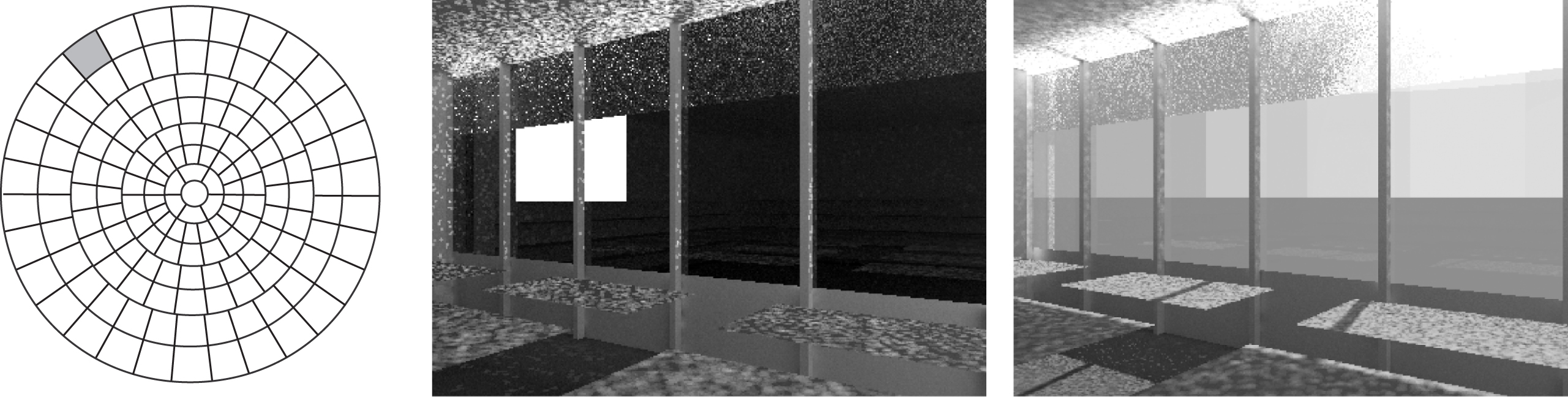
Fig.2
Comparison of the RADIANCE 3 Phase Method sun & sky model (left, with Reinhart subdivision factor 2), the DAYSIM model (second from left, schematic), the RADIANCE 5 Phase Method sun vector (second from right) and the EvalDRC model (right). Only a section of the sky hemisphere is shown.
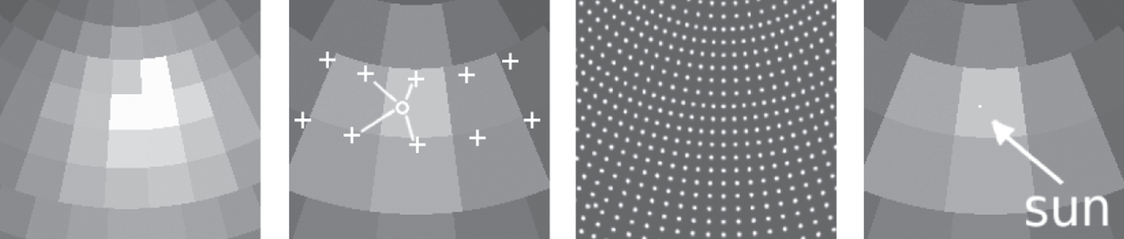
Fig.3
Examples of DRCs and DRC installations. Top left: Interior daylight distribution generated from a functional DRC made of curved specular lamellae integrated into a double glazed window. Top right: Skylight sections of a larger office building with DRCs combining sunlight retroreflection and daylight redirection. Bottom left: Exterior DRC installation with movable louvers. Bottom right: Custom DRC installation for staircase lighting, adding aesthetic dimensions to the pure lighting functionality. Sky and sunlight is redirected through a rectangular short light pipe with facetted mirrors, to produce lighting patterns varying in appearance over the course of a day. Photograph top right: Copyright Osram, Traunreut (Germany), photographs top left and bottom row: Copyright Bartenbach, Aldrans (Austria).
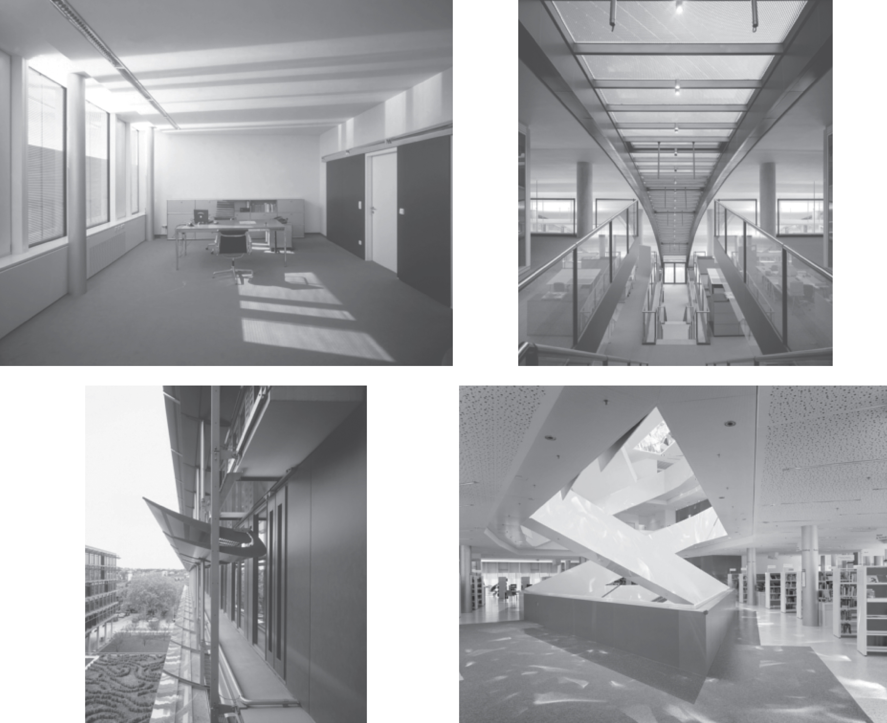
Fig.4
Schematic representation of the transmission part of a BSDF data set. One section pair is highlighted, showing the incoming irradiance from direction (θi, φi) contributing to the outgoing radiance into direction (θ0, φ0). Often, BSDF data is stored at a much higher angular resolution than shown in this schematic drawing.
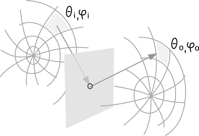
Fig.5
Left: Projection of the scanning paths of a goniophotometer detector head onto a plane. Each grey line consists of closely located points, representing measurement points on a hemisphere on the backside of the sample. The grey disc indicates a local region of high resolution data corresponding to a peak. Right: 3D mountain plot of BTDF data of a redirection system for one incoming light direction, showing light scattering from one incoming direction into different outgoing directions.
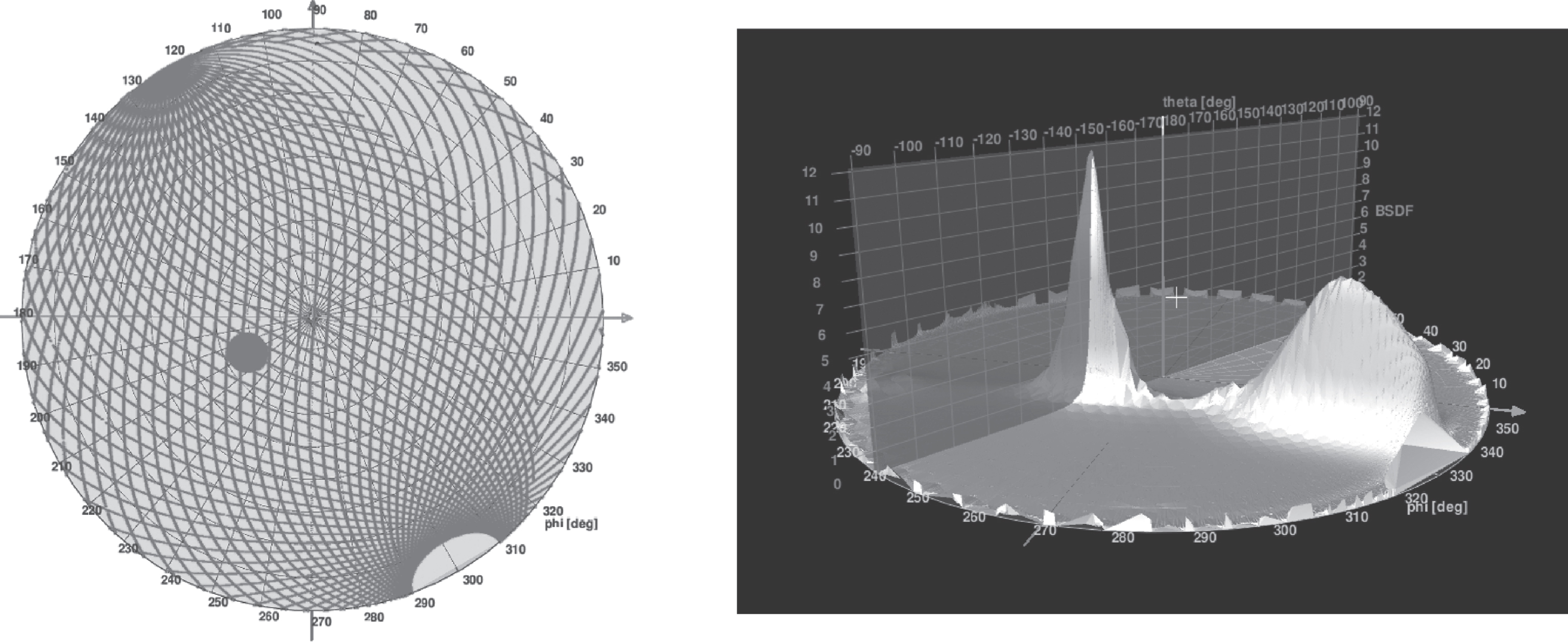
Fig.6
Principle of the Contribution Photon Mapping implementation. Photons emitted from the light sources are deposited as primary photons upon their first hit in the scene. Each spawned photon then references this primary. In the gathering step at point
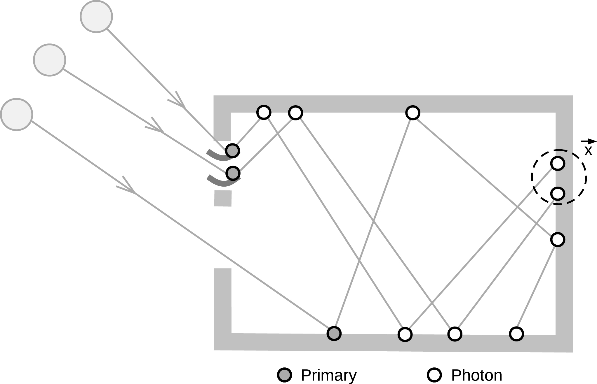
Fig.7
EvalDRC process flow.
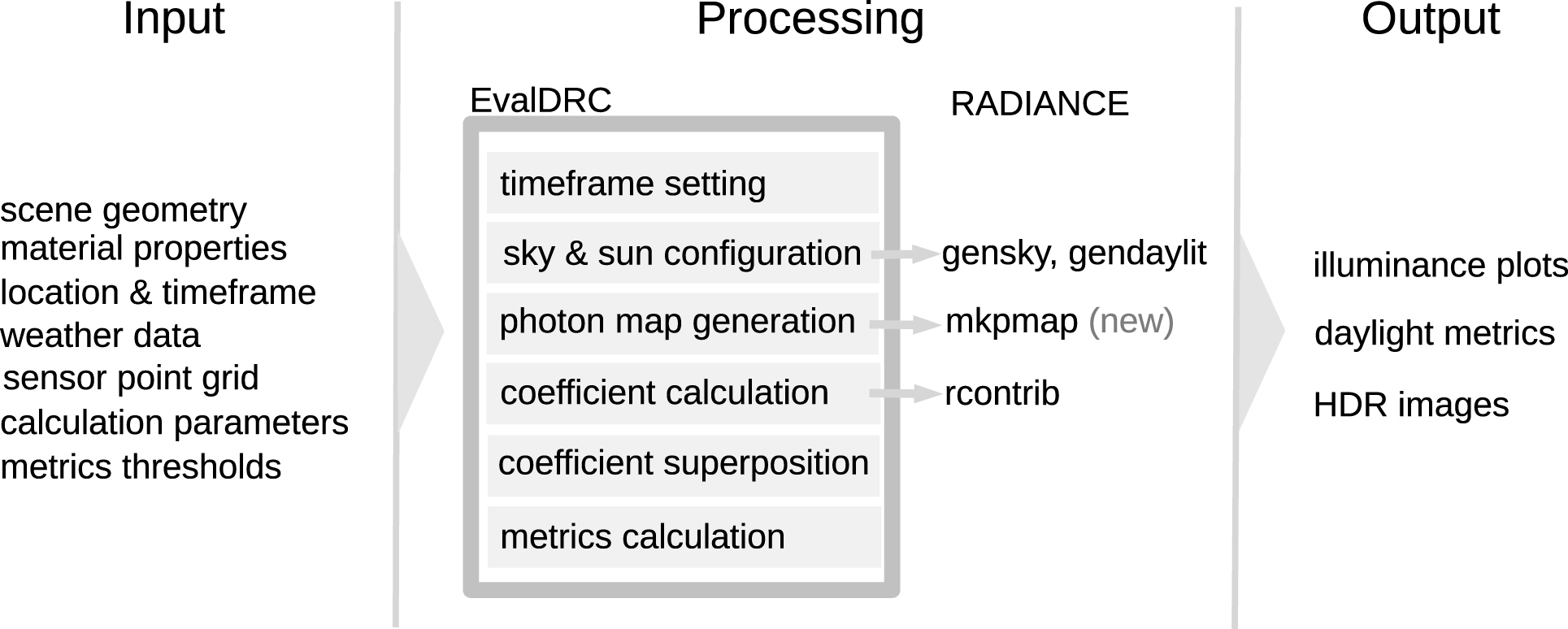
Fig.8
Plan view of the studio classroom used in our case study. The light grey fields indicate the furniture and the dashed line marks the sensor plane for the illuminance calculation. On the right, a photo of the room is shown, taken from the entrance facing the window facade.
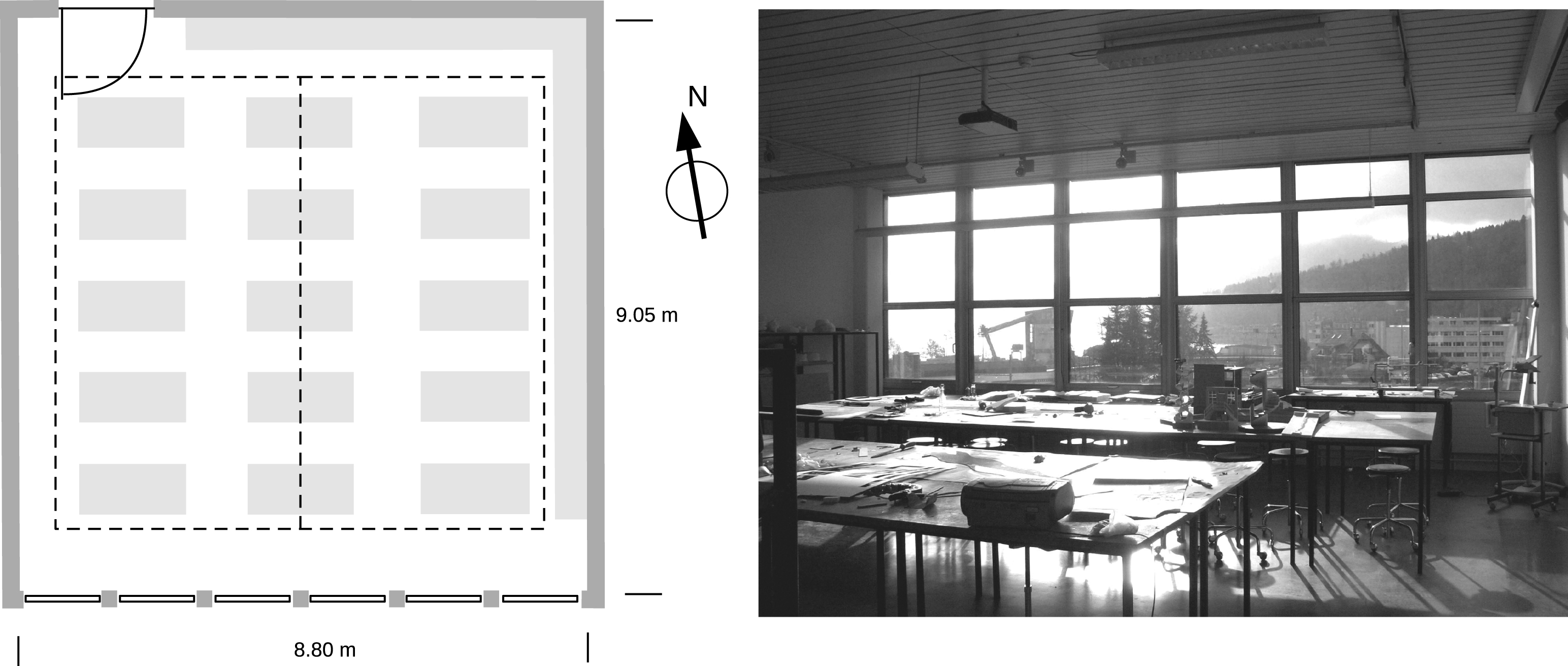
Fig.9
Sample glass plate with a layer of the micro-structured film used in our case study held against a window on a sunny day, showing both the redirection effect on the ceiling and the reduced transmission for the direct view through the sample.

Fig.10
Partitioning of the vertical window segments of the facade in the abstract model used for the simulation. The existing facade is shown on the left, on the right the three optimization variants and their different set-ups with a combination of either wall and clear glazing (O1), DRC and clear glazing (O2) or wall and DRC sections (O3) are depicted.
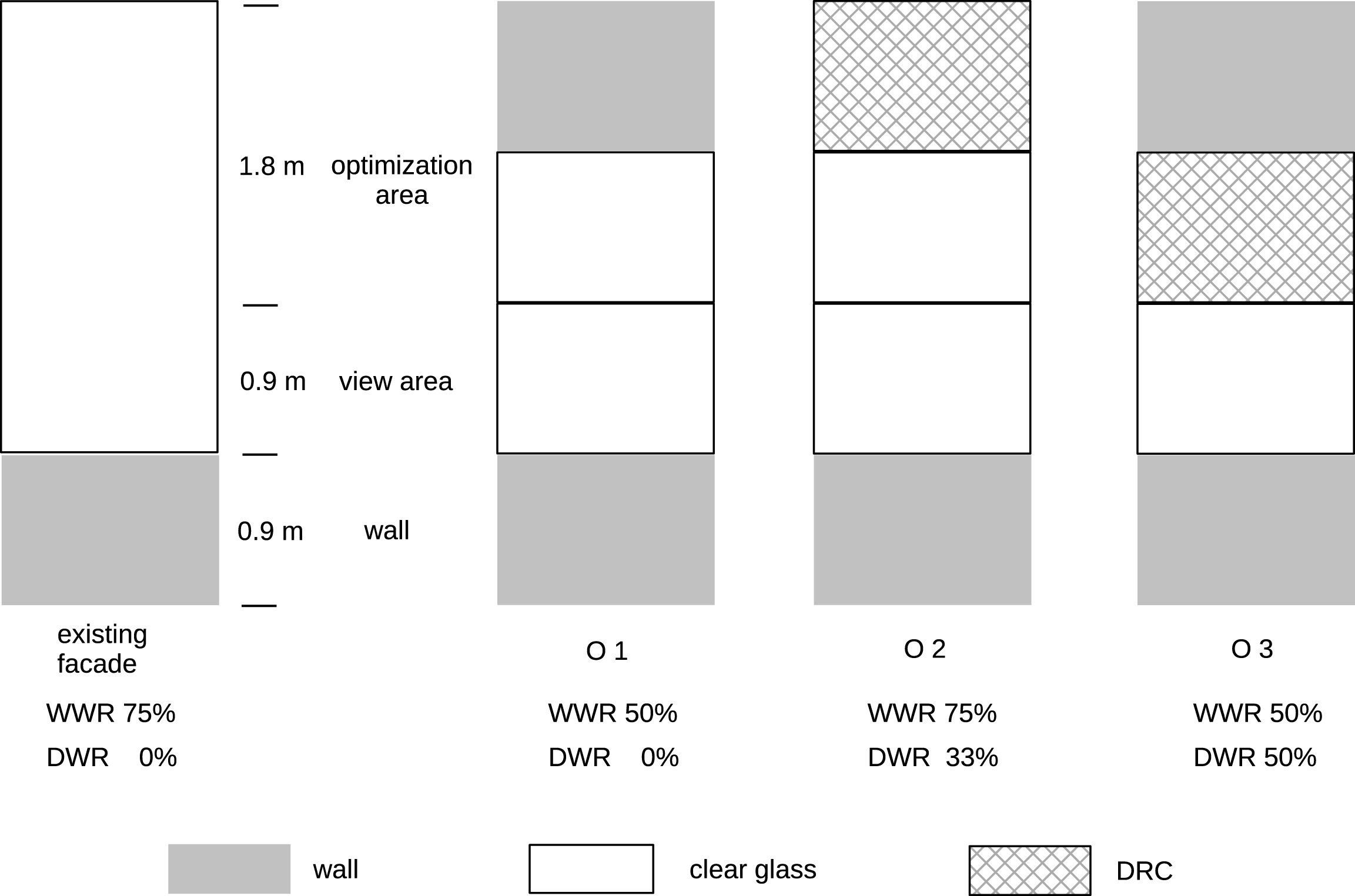
Fig.11
Daylight metric graphs for the existing facade (top left) and the optimization variants O1–O3 (top right and bottom). Each graph shows the annual sDA and ASE in a bar diagram and the new monthly msDA and MSE as line plots. The dashed line shows the monthly percentages of timestamps with active sunshade. Comparing the left and right graph in each row shows the influence of reducing the WWR, whereas comparing the top and bottom graph in each column shows the influence of introducing the DRC.
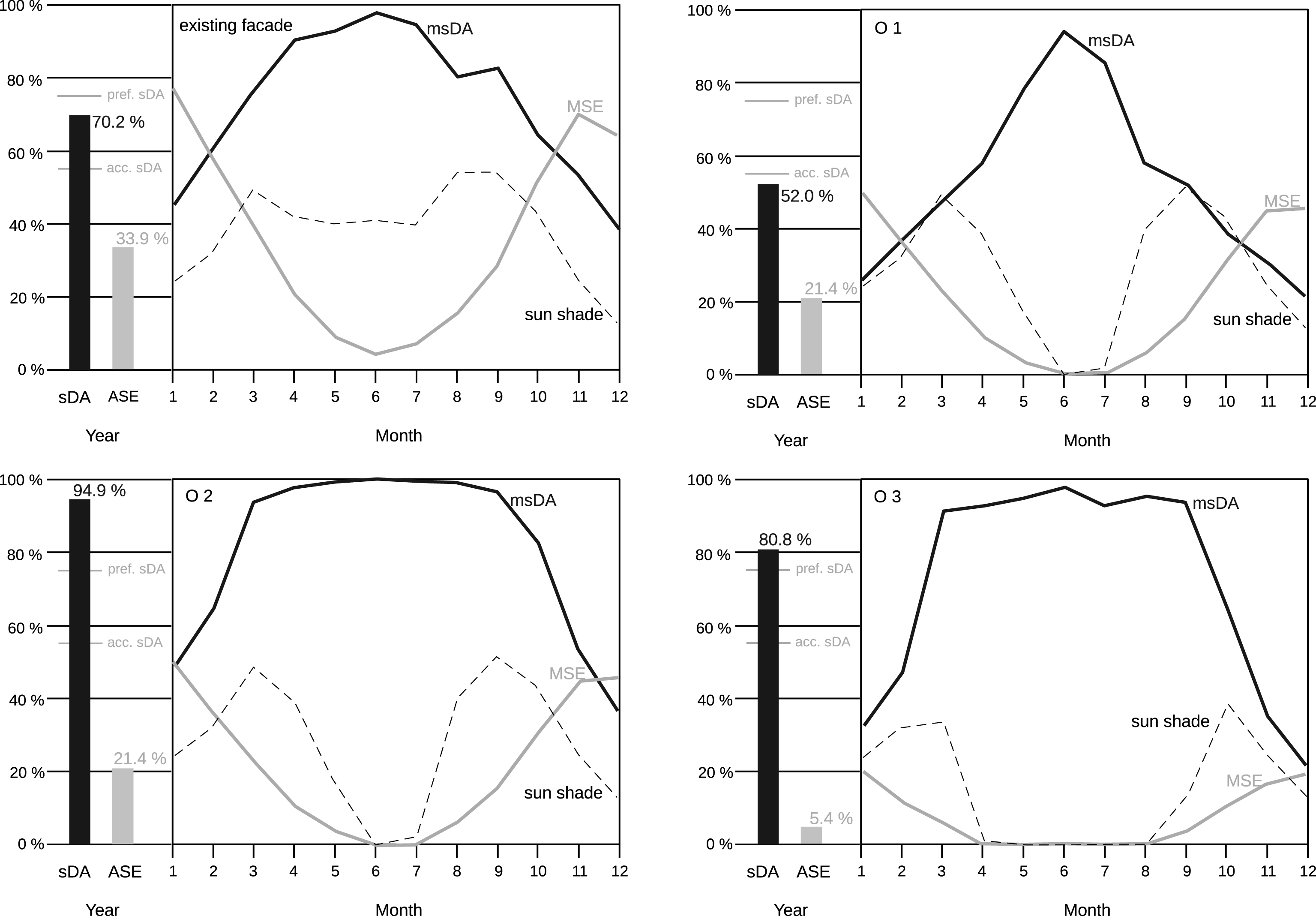
Fig.12
Comparison of msDA graphs (left) and MSE graphs (right) of the variants O1–O3 (continuous and dashed lines) vs. the graph for the existing facade (shaded in grey).
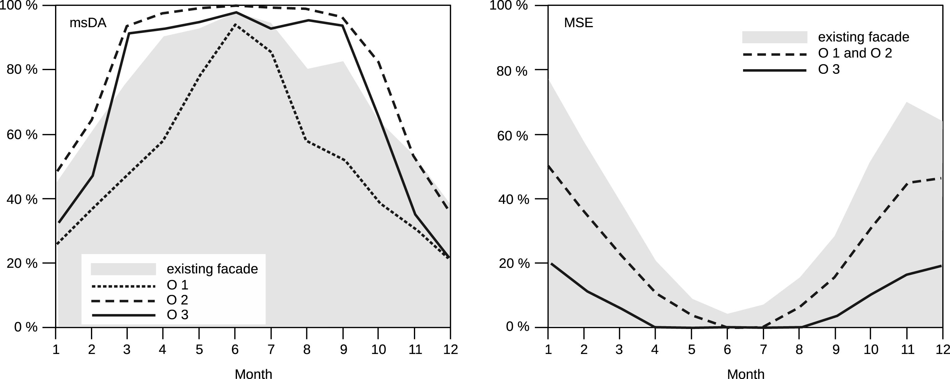
Table 1
Solid angles as initial indicator for potential coefficient size of the daylight sources in decreasing order
| daylight source type | solid angle | typical radiances | |
 | ground reflection | Ω = 2π ≈ 6.28 | ≈2 -20 |
 | one sky patch | Ω ≈ 2π/145 ≈ 0.40 | ≈5 -300 |
 | sun | Ω ≈ 6 .10-5 | ≈3 -5 · 106 |

