
A unified framework for calculating aggregate commodity prices from a census dataset
Abstract
Economic data collection from commodities producers in the United States typically consists of revenues and quantities. While the data collected in some sectors such as fisheries are a census of the population, features of the population such as prices, must be calculated. Unit values are widely used as a price measure to impose a single price in place of dispersed ratios of revenue to quantity from individual producers but alternatives exist. In this paper, different linear aggregation procedures are used to calculate price measures, such as ratio-based calculations (e.g., ratio-of-means, mean-of-ratios), or estimation by ordinary least squares. There are non-trivial differences in the prices calculated depending on the procedure. This paper proposes a unified framework, including Bayesian estimation, for considering the tradeoffs inherent in the different methods commonly employed.
1.Introduction
Price dispersion, which represents deviations from the Law of One Price, is common in transaction data (see Kaplan and Menzio [1]). With variability in the ratio of revenues to quantities among producers, or sellers, what is the appropriate ‘price’ of a commodity such as frozen king crab? The answer to this specific question is important to fishermen because fishery managers collect fees in the Bering Sea based on a standard price, which is a unit value. In this case, data on production and revenues are collected from every commercial fisher and processor that operates in Bering Sea fisheries, and standard prices represent a census of commercial operators in these fisheries. This paper develops alternatives to standard prices to examine effects of price dispersion.
Given cross-sectional data with quantity units and dollar values for any commodity, a first objective is usually to determine a price. But how should this price be calculated? This problem is endemic to low frequency data collection over time or space that include many transactions with dispersed prices because collection efforts will typically focus on aggregates which can be summed, of which two common variables are production quantities and revenue.11 For example, import and export data from the census bureau report only value and volume, but not prices of individual transactions. In some cases, collecting prices over an interval of time may be burdensome because they occur at a transaction level and would be distributed at irregular times over the interval the data are collected. However, medium and high frequency data face similar aggregation problems (e.g., Triplett [2]), and the problem of price dispersion applies to the basic level of aggregation used to construct price indices. Baye [3] formally incorporated price dispersion into price index theory, and his numerical results show the use of mean prices in an index leads to bias.
In general, index number methods break down at some level of disaggregation. Diewert [4] recommended unit value as a suitable price aggregate if data on quantities are available. The practice of using unit values in place of observed prices is widespread (e.g., Reinsdorf [5]; Nevo [6]), but encounters problems if conditions for homogeneity are not met (e.g., Balk [7]).22 Deaton [8] analyzed the bias that arises from using unit values to proxy prices in a demand system. Silver and Webb [9] found evidence of bias in the unit value index when using scanner data to compare effects of different aggregation levels on a consumer price index. According to Bradley [10, p. 41], “Even though it is often used throughout the economics profession and statistical agencies, little research has been done on the use of the unit value as an aggregate price measure or the use of the unit value index as a lower level subgroup price index.” Moreover, Bradley reports on studies of scanner data that use a unit value as a “plugged-in” price measure to impose a single price for an item on an area-month basis, and provides evidence this practice induces specification error and bias.
Mills [11] began his chapter on price dispersion with a description of price relatives varying around a mean value. His description can easily be extended to price levels, with dispersion around a mean price. Hence this paper starts from a related premise where the price level can be viewed as a statistical parameter, or an equivalent price aggregate, such as unit value. Viewed either as a statistical parameter, or astatistical variable, the estimate, or aggregate, gives a scalar that relates quantities to dollar values for the entire population.
This paper follows the example of Balk [7] in questioning when is a set of economic transactions sufficiently homogeneous to warrant the use of unit values. We have production data with revenues and accurate quantities collected annually, i.e., longer than a Hicksian week (Hicks [12, p. 122]), and considerable variability exists in annual revenue to quantity ratios among producers. The methods presented in this paper apply to this type of price dispersion by treating unit values as a type of average price within a family of mean price estimators, with an associated price distribution. We explore this family of estimators, and broaden it to include Bayesian estimation with a prior based on unit value. The application in the paper is to an interesting commodity, frozen Alaskan king crab, but methods in the paper could apply to any commodity for which data on quantity and value are available.
Unit value is the standard method of calculating an aggregate price over an interval of time which in technical terms is a linear aggregation procedure with a quantity weighted-average of per-unit value (i.e., price) for each production unit. This method intentionally integrates out information about the distribution of values among production units (e.g., vessels, processors) to calculate a single number, and the standard method is equivalent to using a ratio-of-means (RoM) (or total value divided by total quantity) to define an aggregate price, which is equal to the unit value. Sometimes, an alternative price is used that is an average per-unit value, which is a mean-of-ratios (MoR).33 If quantity and value data are available for all production units in a population, then both standard and alternative methods calculate ratios that can be interpreted as defensible aggregators for the population of prices. However, the RoM and MoR are not equal except if perfect symmetry prevails, and production volume is equal for all units, which is unrealistic. Furthermore, in practice the difference between the two means can be substantial. When the dataset is a census of the population, what does the application of these ratio-based calculations (and others) imply about the relationship between aggregate value and quantity? These and other estimators can be compared within the context of a statistical framework to determine what parameters are being estimated by these different aggregation methods.
This process implies price is an unknown that is calculated by dividing value by quantity, or equivalently, value is the product of an unknown price and quantity.44 The form of this relationship in a statistical framework suggests value is the response variable, quantity is the explanatory variable, and price is the unknown parameter. The use of regression analysis to estimate prices is a natural outcome of a statistical framework for price estimation, and in this paper, we investigate regression estimates of price relative to the RoM or the MoR within the family of linear aggregation. Under linear regression, the coefficient estimate in the regression of value on quantity is a price estimate which opens up new possibilities for alternative price estimates that control for exogenous factors, including seasonality. However, even a simple regression poses potential problems. For example, ordinary least squares (OLS) estimates are biased if an explanatory variable is correlated with the error term. In this paper, we assume quantity variables are exogenous explanatory variables. This assumption is potentially justifiable in resource extraction and agricultural settings where supply changes are environmentally driven. In the paper, we present some evidence in support of this assumption for our empirical application to frozen king crab, and outline a companion theory where revenues are the explanatory variable, and causality runs from revenues to quantities.
In particular, the inverse demand approach of Barten and Bettendorf [14] is generally accepted for fish and other perishable commodities (e.g., Park et al. [15], Lee and Thunberg [16]). A clear justification often exists for an inverse demand specification that treats quantity as an independent variable in fish price-quantity relationships because the total catch is regulated. However justification for an inverse demand specification can extend beyond management constraints. For perishable goods, Barten and Bettendorf [14, p. 1510] explain “supply is very inelastic in the short run and the producers are virtually price takers” and “price-taking producers and price-taking consumers are linked by traders who select a price which they expect clears the market” from which the conclusion is “causality goes from quantity to price.” For empirical support, Eales et al. [17] compared models of Japanese demand for fish and found the inverse demand specification “dominated” other demand specifications based on testing and forecasting performance. In addition, Hospital and Pan [18, Appendix A-7] describe conditions where price could be exogenous and quantity endogenous. They applied exogeneity tests to price-quantity relationships in this setting and found strong support for the inverse demand specification.
The statistical framework we propose applies to datasets that represent a cross-sectional census of the population and where the objective is to find an accurate measure relating value and quantity (as opposed to finding an optimal index for examining price changes over time). When the data are a census of the population the data contain all features of the population distribution. Because there is no sampling there is no underlying probabilistic mechanism for which population inference must be used.55 If we want average revenues for the population then we can simply calculate the average. We can also calculate the variance of the population. However, average in this context has no variance, it is simply the average. For price, an aggregate is less obvious because price is a rate variable which relates the flow from the quantity produced to revenues of a particular market transaction. The aggregation of the rate can depend on the importance or significance of the transaction (e.g., prices from high volume transactions may be more important in the aggregate price) which in turn relates to the aggregation methods used on quantities and revenue. Conceptually related is the property of factor reversal in economic indices, which is satisfied when the same index method is used to create price and quantity indices that capture changes in the ratio of values (see Coelli et al. [19]).
We can still conceptually impose a statistical model on census data by hypothesizing a superpopulation. Within a statistical framework, a RoM and a MoR can be compared if they are treated as two different estimators of an unknown superpopulation parameter (see Godambe and Thompson [20]). Within the superpopulation model an OLS regression of values on quantities can also be considered as an estimate of the aggregate price. From a statistical standpoint, if the assumptions for OLS are satisfied then the coefficient on quantity is an unbiased estimate of the marginal change in revenues with respect to quantity; that is the price. In addition to OLS, this paper proposes Bayesian linear regression which recognizes that prices have a distribution and allows the researcher to incorporate prior beliefs about the distribution of prices.
There are critical distinctions between the aggregate price formulae discussed here and price indices, which have been the focus of much of the price index literature. The aggregate price formulae presented here (which relate value and quantity) are not price indices (which relate prices over time/space). The construction of an aggregate price can be thought of as analogous to the construction of an index. As with indices there are numerous formulae available to choose from even for a basic object such as quantity. However, an aggregate price and a price index differ in some fundamentally important ways. The most trivial difference is that an aggregate price retains the scale of dollars per-unit quantity while indices are unit-less by design. More importantly, indices are designed to compare the prices in one state relative to another (generally one time period to another), while an aggregate price summarizes prices in a single state (i.e., at a point in, or interval of, time) for the purpose of obtaining an objective measure relating aggregate quantity and value. Because of this, when the objective of analysis is price change (e.g., over time/space) then price indices are the preferred metric. Moreover, price indices may rely on aggregate prices calculated using methods in this paper.
To demonstrate the potential differences associated with alternative aggregation procedures, we present three price estimators in a case study of the first-wholesale price of Alaska red king crab (Paralithodes camtschaticus). This case is interesting because the price of red king crab is historically variable, and the Alaska red king crab fishery is a commercially important industry to both Alaska and Washington state (Garber-Yonts and Lee [13]). The red king crab fishery is one of the largest crab fisheries in Alaska comprising roughly 20% of the total economic value from crab harvest. The Bristol Bay red king crab (BBRKC) stock constitutes roughly 95% of the red king crab harvest and is the focus of the empirical analysis. In particular, the first-wholesale price of red king crab is estimated from Alaska Department of Fish and Game (ADFG) Commercial Operator’s Annual Reports (COAR), an annual census of commercial fish and shellfish processors in Alaska that records annual data on production and first-wholesale revenues.
Although the fishery is open from October to January, the BBRKC fishery primarily harvests in November of each year.66 The majority of sales occur in November in anticipation of the holiday season. King crab is more of a seasonal specialty good than a high volume commodity, such as whitefish fish fillets, which can contribute to price dispersion. The main product after processing is packaged sections (e.g., whole crab legs) of cooked and frozen king crab meat in the shell. The flavor and texture of king crab meat cooked and frozen in the shell is reported to deteriorate after about 6 months in cold storage (Dassow [21]).
Cooked and frozen king crab sections may be exported for finishing or finished domestically. Though the share varies annually, exports typically constitute roughly half of the production volume. The largest importer is Japan followed by Korea, Canada, China, and Western Europe (Dalton and Lee [22]). Smaller but steady markets exist in tourist destinations including Mexico, the Caribbean, and Southeast Asia where in Indonesia some additional processing occurs for export back to the U.S. The U.S. imports much more king crab than it consumes from domestic production. In global markets, the BBRKC fishery competes mainly with Russian red king crab fisheries in the Bering Sea, and in the Barents Sea. Historically, Russia has been the largest global supplier of red king crab. Norway is also a global supplier.
The BBRKC fishery was closed in 1994 and 1995, but recovered before rationalization in 2005 (Kruse et al. [23]). In 2011–13, the BBRKC fishery produced an annual average of 5.9 million pounds of finished products, and over this period, was estimated to have generated average real first-wholesale revenues (i.e., revenues received by processors at the first sale of finished products) of about $78.5 million per year (Garber-Yonts and Lee [13, Table 1]). The BBRKC stock was included in the BSAI Crab Rationalization Program.77 The fishery for BBRKC is managed cooperatively by the NMFS, the North Pacific Fishery Management Council (NPFMC), and the State of Alaska. Management of BBRKC is based on a stock assessment model that is used to estimate an Overfishing Limit (OFL), the level of catch that corresponds to a proxy for the fishing mortality rate which achieves Maximum Sustainable Yield (MSY).88 The Acceptable Biological Catch is an OFL buffer that accounts for uncertainty and ensures the probability of exceeding the OFL is less than 50%, and is used as an upper bound for the total allowable catch (TAC), which in turn determines the market supply of BBRKC.
The outline of this paper is as follows: Section 2 describes a superpopulation model and estimation methods based on linear aggregation that relate production quantities and values. Section 3 presents a Bayesian estimation method and compares its results with those based on linear aggregation. Section 4 concludes with a discussion of results.
2.Linear aggregation and regression
In practice, ex-vessel and first-wholesale prices for fish are calculated with each cross-sectional year treated as a separate (and independent) sample. This paper adopts that practice, and to save notation, the subscript for time
2.1Astatistical calculations of an aggregate price
Even in a framework that does not rely on a statistical foundation a calculation must be constructed to meet some objective to be meaningful. By extension from the observation by observation case, a natural objective is to construct an aggregate scalar price
(1)
where
As an example, consider price calculated by using summation for the aggregator function
This calculation is ratio of average value and average quantity, the RoM. The RoM can also be written as a quantity-weighted arithmetic average price,
(2)
where
2.1.1Generalized astatistical methods
The formulation proposed in Eq. (1) reduces the problem to choosing an aggregator function for prices and quantities. The weighted generalized mean or power mean,
Conservation of the value-price-quantity relationship (Eq. (1)) under the weighted generalized mean aggregator results in the implicit formula for price:
The generalized aggregate price function is the ratio of the weighted generalized means of value and quantity,
(3)
Thus, treating all observed values and quantities equally
(4)
Alternatively, giving preference to observations with smaller values by using
Taking the unweighted geometric mean of value and quantity,
which is sometimes used in productivity analysis and instances where the log-linear arithmetic average of prices might be the preferred.
Arranging the generalized aggregate price function to isolate observation level prices shows that it can be generically cast as either a quantity-weighted generalized mean or a value-weighted generalized harmonic mean,
(5)
The quantity-weighted generalized mean representation is a more economically intuitive functional form than the harmonic mean. Furthermore, value is typically viewed as the result of an interaction between price and quantity. Because of this, if weights are constructed as functions, then basing weights on quantity should be preferred to value. In practice, weights can be based on anything that can be reasonably justified to meet the objectives of the analysis for which the price is being constructed. However, for all but the most common calculations of an aggregate mean the choice of weights should be made explicit.
The generalized aggregate price function and consideration of its parameters shows that the most objective calculation of the price is the ratio of means,
2.2Statistical estimation of an aggregate price
A statistical framework is used when there is some underlying probability mechanism that is producing the observed data. When calculating population parameters sampling is often the probabilistic mechanism. There are many tools within statistics that allow all researchers to ask interesting hypothetical questions about the population. When the data are a census of the population, statistics can still be employed by assuming that the observed population is a sample of some larger superpopulation. The statistical methods employed can depend upon the assumed source of random variation and the framework under which the problem is approached.
2.2.1Direct estimation
If we take as given that
Consider the model for price where
When the variance is heteroskedastic, a weighted average is the optimal (minimum variance and MLE) unbiased estimator of the mean of the price distribution. The weights are the inverse of the variances,
(6)
This may be justified in the case where smaller trades may be associated with a higher variance as in a commodities market. One way of capturing this relationship is by hypothesizing that the variance is proportional to inverse powers of quantity,
Thus, in the statistical case the choice estimator can be represented as the analyst’s belief about the relationship between the variance and the quantity. When the variance is constant,
(7)
Other estimators can be devised as well through different choices of
2.2.2Estimation by regression
When the object of analysis is the prediction of value for hypothetical quantities, regression is a more appropriate statistical tool. The notion that the actual price paid in the market is random with a distribution is more consistent with Bayesian framework (in contrast to classical regression where quantity is related to value through a constant but unknown price),
where
When the normal distribution is used for the likelihood and prior distributions have a known variance and a diffuse prior, or the sample size is sufficiently large, then the estimate of the posterior mean of the price is the OLS estimator,1212
Interestingly, the OLS estimator itself is also a quantity-weighted average of price with quadratic weight on quantity. Equation (8) shows a connection between the direct statistical estimation of price in Section 2.2.1 and the regression estimator. A general representation of the statistical estimators is the power weighted average:
(8)
By analogy to the weighted average, heteroskedasticity (e.g.,
3.Empirical comparisons of aggregate price estimates
Each year the National Marine Fisheries Service (NMFS) is responsible for publishing standard prices to determine ex-vessel value for the assessment of cost-recovery fees in various catch share programs.1313 For example, NMFS standard prices are used to assess fees for observer coverage in North Pacific groundfish fisheries (77 FR 70062), and these standard prices are based on the RoM using 3-year moving averages of volume and value (80 FR 77606). The use of 3-year moving averages is intended to dampen inter-annual variability in standard prices. As stated in the introduction, our empirical application uses data for red king crab from the BBRKC fishery. Although NMFS does not currently publish standard prices for Alaska crab stocks, the question posed at the beginning of the paper about which price estimate to use for the standard price is relevant and informed by comparing price estimates in this paper.
First-wholesale data on aggregate annual production quantity and revenue for the BBRKC fishery were obtained from the Alaska Department of Fish and Game Commercial Operator’s Annual Reports (COAR). The COAR is collected annually from processors in Alaska. These annual data comprise sales from between 15 and 21 processors processing crab between 2010 and 2014. Using these data we compare nine different price estimates in five cross-sections (across processor) of wholesale value and production data within the years 2010–14. As explained in the introduction, we assume quantity variables are exogenous explanatory variables, and follow Hospital and Pan [17] by applying exogeneity tests to price-quantity relationships.1414
The first three estimates are the ratio estimators and OLS (Table 1). The differences among these price estimators are larger in some years than others. In 2011, the MoR and OLS differed by less than 1%, and slightly more than 10%, respectively, relative to the standard RoM. In addition, OLS differed by more than 6% in 2014. Relative differences are less than 5% for OLS in other years. The largest relative difference for MoR is 7% in 2012, with relative differences of less than 5% in other years.
Table 1
Comparison of price estimates by ratio-of-means (RoM), mean-of-ratios (MoR), and ordinary least squares (OLS), for Alaskan Red king Crab 2010–2014
| YEAR | RoM | MoR | OLS |
|---|---|---|---|
| 2010 | 13.58 | 13.53 | 13.27 |
| 2011 | 17.62 | 17.72 | 15.84 |
| 2012 | 14.88 | 13.84 | 15.51 |
| 2013 | 12.59 | 12.02 | 13.06 |
| 2014 | 11.59 | 11.14 | 12.34 |
The other six price estimators come from Bayesian estimation, three from the normal regression model, and the other three from the lognormal model. The three are maximum likelihood, mode of the pdfs, and posterior mean. Bayesian price estimates treat the error variance as a nuisance parameter to concentrate on a Bayesian analysis of price estimates. The maximum prior probability density function (pdf) was set to the RoM for all estimates. The first model is the linear model
(9)
Inserting the maximum likelihood estimate of the error variance
Extending the estimation method to a fuller treatment of uncertainty in the error variance can be simple depending on the nature of the data and assumptions. The posterior distribution is proportional to the concentrated likelihood times the prior pdf,
(10)
The error variance formula in the concentrated likelihood is
Table 2 presents point estimates from the regressions with normal and lognormal models. Attention is focused on the point estimates in Table 2 for direct comparison with the astatistical interpretation of unit value calculations for a census dataset in Table 1.
Table 2
Comparison of price estimates by normal and lognormal regression models based on the maximum prior (
| YEAR | MAXPRI | MAXLIKE | MAXPOST | EXPOST |
|---|---|---|---|---|
| Normal | ||||
| 2010 | 13.58 | 14.32 | 13.74 | 13.73 |
| 2011 | 17.62 | 17.53 | 17.60 | 17.60 |
| 2012 | 14.88 | 16.27 | 15.14 | 15.14 |
| 2013 | 12.59 | 13.73 | 12.89 | 12.88 |
| 2014 | 11.59 | 12.82 | 11.92 | 11.91 |
| Lognormal | ||||
| 2010 | 13.58 | 13.15 | 13.23 | 13.24 |
| 2011 | 17.62 | 17.40 | 17.43 | 17.48 |
| 2012 | 14.88 | 13.60 | 13.76 | 13.78 |
| 2013 | 12.59 | 11.70 | 11.84 | 11.86 |
| 2014 | 11.59 | 10.78 | 10.95 | 10.97 |
Table 3
Summary statistics of the price estimates, for Alaskan red king crab 2010–2014
| Year | Processor | Min | Max | Average | Range | Standard | Coefficient |
|---|---|---|---|---|---|---|---|
| count | deviation | of variation | |||||
| 2010 | 15 | 13.15 | 14.32 | 13.53 | 1.17 | 0.370 | 0.027 |
| 2011 | 21 | 15.84 | 17.72 | 17.36 | 1.88 | 0.578 | 0.033 |
| 2012 | 17 | 13.6 | 16.27 | 14.66 | 2.67 | 0.949 | 0.065 |
| 2013 | 19 | 11.7 | 13.73 | 12.51 | 2.03 | 0.693 | 0.055 |
| 2014 | 17 | 10.78 | 12.82 | 11.60 | 2.04 | 0.702 | 0.060 |
Figure 1.
Normalized histograms and estimated pdfs for normal and lognormal models of red king crab price estimates 2010–2014 (prior
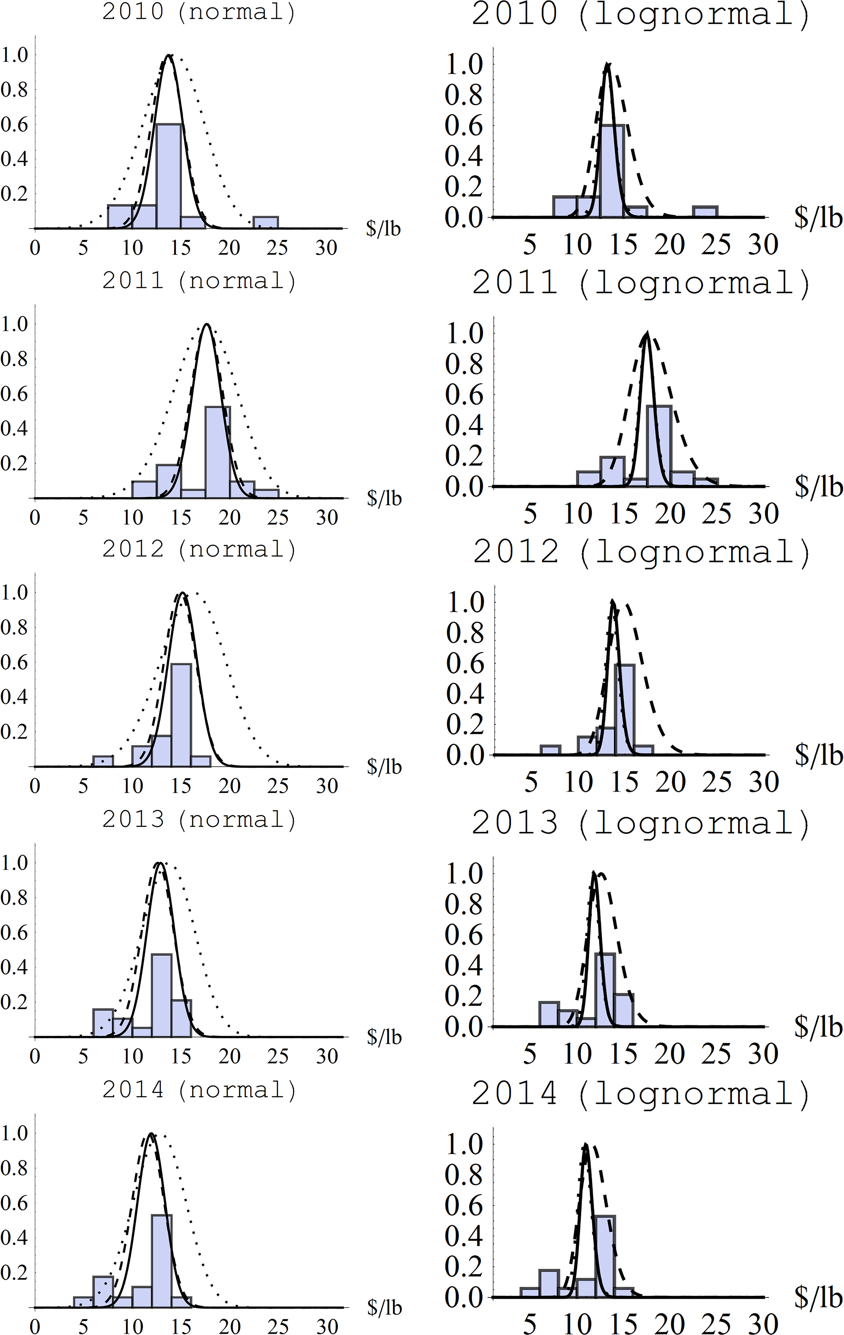
Figure 2.
Comparison of price estimates by RoM, MoR, and OLS, with normal and lognormal regression model estimators MAXLIKE, MAXPOST, and EXPOST, for Alaskan red king crab 2010–2014.
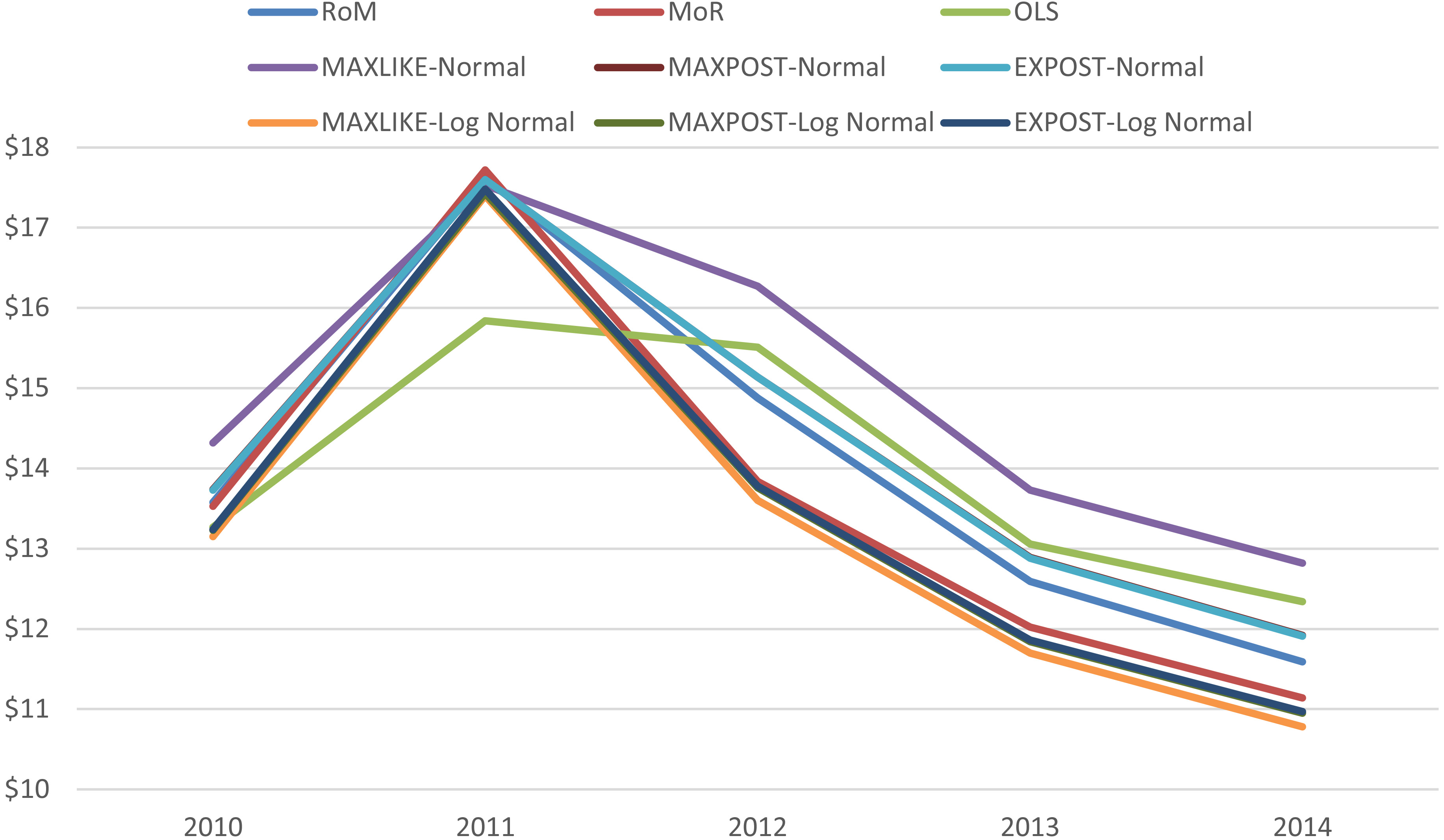
Figure 1 summarizes results of the Bayesian estimation by showing probability-normalized histograms of the cross-section for each year, and presents uncertainty with plots of pdfs for the likelihoods, priors, and posteriors. Results of the Bayesian estimation, and other numerical results in the paper, such as the OLS regressions and endogeneity tests in Wooldridge [25, Ch.15], were computed in Mathematica 8 for Microsoft Windows (64-bit) running on an Intel core i7 CPU at 2.67 GHz and 6 GB of RAM. Mathematica’s NMinimize and NMaximize functions were used for least-squares and maximum likelihood operations, respectively, and NIntegrate was used to evaluate integrals that form the mean of the Bayesian posterior distributions.
In all cases, differences between the maximum posterior and posterior mean are relatively small and almost negligible for the normal regression model. The OLS and maximum likelihood estimates are not equal because of the concentrated likelihood. The maximum likelihood price estimates for the normal regression model are larger than the other estimates in most years. The biggest discrepancy in price estimates is OLS in 2011 which is substantially less than the other estimates that are relatively close together. The low OLS price estimate in 2011 is due to the bi-modal mass (evident in the histograms presented in Fig. 1) amplified by the quadratic weight on quantity in the OLS formula.
In general, differences between the maximum likelihood and maximum posterior estimates were larger for the normal regression model than the lognormal model. An interesting result is that the maximum posterior for the normal regression model is closest to the RoM, and the maximum posterior for the lognormal model is closest to the MoR. This relationship provides an interpretation for each (i.e., normal and lognormal) Bayesian estimate. For this particular dataset, it is never the case that the choice of method results in a change in sign for the year-over-year changes in price (Fig. 2). In theory, choice of weights associated with different methods could produce this result. Tables 1 and 2 show the range of estimates for price is quite large.
Summary statistics for the price estimates are presented in Table 3. For example in 2010, the difference between the smallest and largest price estimates was $1.17/lb (a 9% change), and in 2012, it was $2.67/lb (a 20% change). Dispersion across the nine estimated prices, measured by the coefficient of variation, was largest in 2012. The maximum likelihood methods tended to produce estimates of the extremes, with the normal tending to produce the largest price estimate and the log-normal the smallest. Excluding these, the range of price estimates in 2010 is $0.31/lb (a 2% change) and in 2012 is $1.67/lb (an 11% change) (Table 1).
4.Conclusion
The method used to calculate an aggregate price from quantity and value data of a cross section is not trivial. Different methods, each defensible based on context, can lead to substantially different estimates of the price. Aggregate price differences such as these can potentially have considerable impact on estimated welfare effects and or price induced incentives, and could affect cost recovery fees collected by NMFS for observer coverage. This paper has considered unifying frameworks for astatistical and statistical calculation of an aggregate price which make explicit the choices made when selecting a method. Select methods for calculating price are compared empirically displaying the marked differences in price the different methods yield which highlights the importance of thinking through the method used for calculating an aggregate price.
Within the astatistical framework (when the data are a census of the population considered) for calculating an aggregate price, a generalized unified pricing function is used to reduce the problem of selecting a method to that of selecting a set of weights on value and quantity and an aggregation parameter. The unified framework shows that the most objective method for calculating a price is RoM (unit value) in the sense that quantity and value are weighted equally and aggregation is linear. The choice of weights and whether to use a ratio of means, mean of ratios, geometric mean, or some other alternative are ultimately a decision for an analyst and can be justified based on context. The unified framework in this paper facilitates comparison among standard and alternative price estimates making these decisions explicit by deriving everything from first principles.
The statistical framework is appropriate when a probability distribution is a real (e.g., data are sampled) or imposed (e.g., hypotheses are being tested) feature of the data. A unified analysis of statistical methods for aggregating prices shows there are potentially important differences among the statistical averages and regression-based price estimates. The quadratic weight on quantity in the OLS price estimates is a potentially unappealing property because of the influence of outliers which can occur for non-informative reasons (e.g., database errors). Furthermore, OLS does not explicitly account for the distribution of individual prices within a dataset. The Bayesian estimation method explicitly models the distribution of prices and can therefore better represent uncertainty. Bayesian estimation delivers pdfs that summarize the individual prices, and these pdfs can be used to derive probabilistic interpretations for the utility or loss associated with different outcomes.
Fundamentally, the purpose of this paper is to recognize that the calculation of a seemingly elementary aggregate price is not a priori elementary, that different aggregation methods can produce substantially different results, and to motivate a moment’s pause before calculating an aggregate price. Furthermore, we seek to inform the questions that served as the impetus for some of the comments by Diewert [4] and Balk [7], which we summarize as, “What aggregation formula should we use to calculate an aggregate price?” While certain estimates of an aggregate price may be justified based on context, defensible methods can differ depending on whether the aggregate price sought is a summary statistic of the data, a parameter of a probability distribution, or the marginal effect on value from quantity. There will arise contexts where it is not clear which aggregation is appropriate, leaving the researcher considerable liberty to consider and defend the use of a given estimator. A purpose of this article has been to provide a framework that lays bare the tradeoffs made by different estimators to help inform their choice.
Notes
1 Low frequency refers to an interval of time or space over which multiple transactions take place at significantly different prices such that the Law of One Price is plausibly violated and as a consequence price dispersion exists.
2 Balk [7] showed that the unit value index fails the identity test unless both base period and reference period quantities are equal, and it fails the dimensionality test and can be sensitive the choice of units. Hence the unit value index is not a true price index.
3 For example, see Garber-Yonts and Lee [13, Table 4.5] where both ratio-of-means (RoM) and mean-of-ratios (MoR) statistics (including the standard deviation for the MoR as a simple measure of distributional variation) are presented.
4 Depending on the data collection value and quantities may not represent a single transaction. It could be multiple transactions within an interval of time with differing prices.
5 This also assumes that the data collection methodology itself does not introduce uncertainty (e.g., measurement error) or that it is negligible. Furthermore, uncertainty arising from the data collection methodology should generally be addressed explicitly and may be dealt with differently than uncertainty from sampling.
7 A voluntary cooperative IFQ program was implemented in 2005 to allocate BSAI crab resources among harvesters, processors, and coastal communities (www.npfmc.org/crabrationalization).
8 See Amendment 24 to the Fishery Management Plan for BSAI King and Tanner Crabs. Current guidelines from the National Marine Fisheries Service for National Standard 1 state “The Magnuson-Stevens Act establishes MSY as the basis for fishery management” (50 C.F.R.
9 As an extreme example, consider two companies one with 90% of the market share and goods priced at $0.50 and the other with 10% market share and goods priced at $1.00. The weighted average of prices is $0.55, and the simple average is $0.75.
10 Note that because the weights appear in both the numerator and denominator and the generalized mean is homogenous of degree 1, normalization of the weights so that
11 The geometric mean is obtained from Eq. (3) in the limit as
12 The variance can also be given a distribution and estimated like the mean. Under similar assumptions the same results hold. The current setup maintains the focus on the formula for the mean.
13 For example, see
14 The endogeneity test in Wooldridge [25, Ch.15], which is based on the t-statistic for an estimated coefficient on residuals from an auxiliary regression with lagged quantity as the instrument, was applied to data used in this paper. This test was applied to the specification used in this paper, with quantity as the explanatory variable and value as the response, and also applied to the inverse specification that treats value as the explanatory variable and quantity as the response. Test results for 2010–2014 reject (5% significance level) the null of exogeneity for quantity in 2011 and 2012. For data used in this paper, the conclusion from these tests is endogeneity in quantity variables is not a problem in most years. With these mixed empirical results in mind, microeconomic theory favors the inverse demand approach of Barten and Bettendorf [14] where producers and consumers are price takers and traders choose prices to clear the market so that causality runs from quantity to price.
15 A lognormal prior
Acknowledgments
We thank the editor and an anonymous referee for helpful comments. The findings and conclusions in the paper are those of the authors and do not necessarily represent the views of the National Marine Fisheries Service, NOAA.
References
[1] | Kaplan, G. and Menzio, G. The morphology of price dispersion. International Economic Review. (2015) ; 56: : 1-42. |
[2] | Triplett, J.E. Using scanner data in consumer price indexes. Some neglected conceptual considerations. In: Feenstra, R.C. and Shapiro, M.D. (eds). Scanner Data and Price Indexes. University of Chicago Press; (2003) . |
[3] | Baye, M.R. Price dispersion and functional price indices. Econometrica. (1985) ; 53: : 217-224. |
[4] | Diewert, W.E. Axiomatic and economic approaches to elementary price indexes. NBER Working Paper No. 5104; (1995) . |
[5] | Reinsdorf, M. Using scanner data to construct CPI basic components indexes. Journal of Business and Economic Statistics. (1999) ; 17: : 152-160. |
[6] | Nevo, A. Measuring market power in the ready to eat cereal industry. Econometrica. (2001) ; 69: : 307-342. |
[7] | Balk, B.M. On the use of unit value indices as consumer price subindices. In: Lane, W. (ed). Proceedings of the Fourth Meeting of the International Working Group on Price Indices. Washington, D.C.: U.S. Department of Labor; (1999) . |
[8] | Deaton, A. Quality, quantity, and spatial variation of price. American Economic Review. (1988) ; 78: : 418-430. |
[9] | Silver, M. and Webb, B. The measurement of inflation: aggregation at the basic level. Journal of Economic and Social Measurement. (2002) ; 28: : 21-35. |
[10] | Bradley, R. Pitfalls of using unit values as a price measure or price index. Journal of Economic and Social Measurement. (2005) ; 30: : 39-61. |
[11] | Mills, F.C. The Behavior of Prices. National Bureau of Economic Research (NBER); (1927) . |
[12] | Hicks, J.R. Value and Capital, Second Edition, Oxford: Clarendon Press; (1946) . |
[13] | Garber-Yonts, B. and Lee, J. Stock Assessment and Fishery Evaluation Report for King and Tanner Crab Fisheries of the Bering Sea and Aleutian Islands Regions: Economic Status of the BSAI Crab Fisheries 2015. North Pacific Fisheries Management Council; January (2016) . |
[14] | Barten, A.P. and Bettendorf, L.J. Price formation of fish: an application of an inverse demand system. European Economic Review. (1989) ; 33: : 1509-1525. |
[15] | Park, H., Thurman, W.N. and Easley, J.E. Modeling inverse demands for fish: empirical welfare measurement in Gulf and South Atlantic fisheries. Marine Resource Economics. (2004) ; 19: : 333-351. |
[16] | Lee, M. and Thunberg, E. An inverse demand system for New England groundfish: welfare analysis of the transition to catch share management. American Journal of Agricultural Economics. (2013) ; 95: : 1178-1195. |
[17] | Eales, J., Durham, C. and Wessells, C.R. Generalized models of Japanese demand for fish. American Journal of Agricultural Economics. (1997) ; 79: : 1153-1163. |
[18] | Hospital, J. and Pan. M. Demand for Hawaii bottomfish revisited: incorporating economics into total allowable catch management. U.S. Department of Commerce, NOAA Tech. Memo. NOAA-TM-NMFS-PIFSC-20; (2009) . |
[19] | Coelli, T.J., Rao, D.S.P., O’Donnell, C.J. and Battese, G.E. An introduction to efficiency and productivity analysis. Springer Science & Business Media; (2005) . |
[20] | Godambe, V.P. and Thompson, M.E. Parameters of superpopulation and survey population: Their relationships and estimation. International Statistical Review. (1986) ; 54: : 127-138. |
[21] | Dassow, J.A. Freezing and canning king crab. Fishery Leaflet 374. U.S. Fish and Wildlife Service. (1950) . |
[22] | Dalton, M. and Lee, J. Alaska fisheries and global trade: red king crab, Paralithodes camtschaticus; sockeye salmon, Oncorhynchus nerka; and walleye pollock, Gadus chalcogrammus. Marine Fisheries Review. (2015) ; 77: (3): 84-90. |
[23] | Kruse, G.H., Zheng, J. and Stram, D.L. Recovery of the Bristol Bay stock of red king crabs under a rebuilding plan. ICES Journal of Marine Science. (2010) ; 67: : 1866-1874. |
[24] | Kleinbergen, F. and Zivot, E. Bayesian and classical approaches to instrumental variable regression. Journal of Econometrics. (2003) ; 114: : 29-72. |
[25] | Wooldridge, J.M. Introductory econometrics: a modern approach. Mason, OH: Thomson/South-Western; (2006) . |


