
An improved definition of official excess winter mortality statistics as the basis for detailed analysis and monitoring
Abstract
In official statistics, excess winter mortality, the number of additional deaths in a winter period, is typically defined as the difference between mortality in a winter period relative to the nonwinter periods before and after. We note two limitations of this approach: (1) the data for the period after winter is available only later, so estimates of excess winter mortality are not timely; (2) unusually high or low numbers of deaths in the non-winter periods can affect estimates. We propose an alternative statistic based on the application of standard seasonal adjustment procedures. We compare the approaches and present some illustrative analyses. The new statistic provides a more objective and timely official series, but is susceptible to revisions, which are shown to be small in practice. We recommend it as the basis of more detailed monitoring and modelling.

1.Introduction
In temperate parts of the world, it has long been recognised that mortality is higher during the winter than at other times of year [1, 2]. There has been considerable interest in modelling the relationship between temperatures and mortality, at both high and low temperatures [3, 4, 5, 6, 7, 8]. Although the increase in deaths during winter is a general pattern, in some years there is higher mortality, for example associated with flu outbreaks or recently COVID-19 [9], and official statistics have been developed to monitor and report on excess winter mortality [10] – the number of additional deaths during the winter period relative to some baseline.
Temporal variation in mortality provides a lot of useful information on which to base policy choices and interventions designed to reduce mortality from particular causes. There has been particular interest in periods or events which lead to increased mortality, and this has given rise to a range of statistics which describe these measures and can be used for monitoring and analysis. One such topic has been mortality in the winter period and its association with low temperatures, and the World Health Organisation has gathered information about experiences in a range of countries as a basis for developing actions to reduce mortality with identifiable causes [11, 12]. The European Union also maintains a database of mortality statistics [13].
There has also been interest in the effects of extreme high temperatures on mortality. Such effects tend to be more localised in time than the effects of low temperatures, and therefore a different approach has developed in their measurement, aligned more closely with extreme value theory [3, 14].
A range of researchers have examined the relationships between cold temperature and effects on mortality [2, 4, 5, 15], the effect of heat waves [3, 16, 6, 17] or both [7, 18, 19, 8, 20]. Gasparrini and co-workers in particular have modelled the relationships between winter mortality and temperatures.
In this paper, however, we do not focus on detailed modelling to help the understanding of the relationships between deaths and different conditions, but rather address the challenge facing official statisticians, which is to produce a measure which can be straightforwardly explained and used as a basis for monitoring and policy formulation, and more widely to support users’ needs for winter mortality analysis. The need for these types of statistics has been made much more explicit by the challenges of monitoring the spread of COVID-19.
In the UK most attention has been focused on mortality associated with low temperatures. The Office for National Statistics (ONS) [21] publishes a weekly estimate of deaths, derived from vital events registration systems. This is one of very few weekly official statistics, and this frequency is useful because it allows a quick policy intervention in response to any indication of increased numbers of deaths. The corona virus pandemic of 2020 has given rise to many more weekly statistics as intense interest has been focused on the impact of the necessary restrictions. ONS also produces an annual statistical bulletin on Excess Winter Mortality in England and Wales, which provides an analysis of the generally observed increased number of deaths during winter months. The measures are analysed by different demographic characteristics and regions, and also consider different causes of death, with additional analysis of temperature and influenza data. Comparable statistics are also produced for Scotland [22] and Northern Ireland [23], calculated in the same way.
Excess Winter Mortality (EWM) statistics are produced using a definition which results from an investigation of alternative measures undertaken by Johnson and Griffiths [10]; curiously, they identify the effect of unusually large numbers of deaths in non-winter months, but do not recommend a change in the statistic used for measurement. The definition had been used previously [2, 4, 24] and has been taken up by other authors [15, 19, 25, 26]. The definition is based on the difference in numbers of deaths in a central, winter period, compared with the average number of deaths in the periods immediately before and after:
where
This current measure of EWM has been criticised as potentially biased because of the effect of extreme values in non-winter periods, which might distort analysis of the data and have implications for public health policy [5]. Other measures have been used, explicitly and implicitly. Hajat and Gasparrini [5] use time series regression methods to analyse daily deaths data and conclude that the current measure should be discontinued and an alternative method found that does not suffer from this bias. Hales et al. [27] used data from New Zealand to model differences between deaths in three winter months (Jun, Jul, Aug) and those in three summer months (Dec, Jan, Feb), ignoring spring and autumn. Their definition of excess winter mortality seems to be based on the fitted odds ratio for winter to summer deaths, although they also use a (W – S)/S percentage which corresponds in concept with Fowler et al.’s EWMI [15].
Johnson and Griffiths [10] compare two alternative methods for estimating EWM to the current ONS method. One, a six-month split where April–September estimates are subtracted from those for October–March, and the other excluding autumn and spring periods with June–September (summer) subtracted from December–March (winter), making it more similar to the method adopted by Hales et al. [27]. They concluded that the three methods provide similar results, and suggested that excluding deaths during the spring and autumn months might be an improvement, to avoid artificially decreased EWM, but without recommending a change.
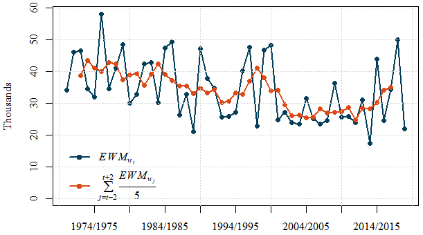
The ONS statistical bulletin, for example Office for National Statistics [21], is typical of official publications on this topic. It reports an estimate of excess winter deaths for the latest year, and typically makes comparisons with other years. It also analyses differences by sex, age group and region. For example, the 2017/18 bulletin reported 50,100 (now revised to 49,410) excess winter deaths and noted that this was the highest since the 1975/76 period. Trends in mortality are also analysed; there can be large annual fluctuations in excess winter deaths, and the ONS uses a simple symmetric five-point moving average of the annual EWM figures as a trend (Fig. 1).
Figure 1.
Excess winter deaths for England and Wales using the ONS measure EWM, and a simple symmetric five point moving average trend.
The rest of the paper is structured as follows. In Section 2 we consider the definition of excess winter mortality, and propose and evaluate target statistics for use by national statistical institutes in publications designed for regular monitoring. In Section 3 we analyse these statistics for England and Wales to demonstrate the effect on inferences from our new approach. Section 4 provides some discussion of the results.
2.Defining a statistic to measure excess winter mortality
2.1Time series decomposition
At face value the expression ‘excess winter mortality’ suggests that we would like to measure the number of deaths which occur additionally during winter compared with some ‘normal’ number of deaths for other periods. The question is therefore how best to construct a reference ‘normal’ number against which the current season’s deaths can be compared. This is not as simple a process as seasonally adjusting the time series of recorded deaths, since in this case the normal winter peak would be detected by the seasonal adjustment algorithm and removed. We can however use the calculated adjustment as a part of our estimate.
Figure 2.
Monthly deaths series for England and Wales (January 1970–July 2019), with seasonally adjusted and trend-cycle estimates.
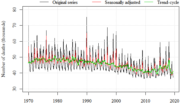
Take as an example the monthly time series of registered deaths in England and Wales (Fig. 2, black/top line). The monthly mortality data are compiled from national daily death occurrences derived from death registrations, available from the latest Excess Winter Mortality Bulletin [21]. This series is clearly seasonal, with peaks in mortality in the winter months. A trend is therefore needed as an estimate of the “normal” number of deaths, and in standard time series decompositions this is called the trend-cycle. If we use 1/2(
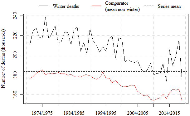
Figure 3.
Number of deaths as a function of winter period (black/top line) and the average of non-winter months (red/bottom line). The dotted line represents the mean number of deaths for the whole span.
A traditional time series decomposition [28] renders an observed time series into three components, the trend T, seasonal S and irregular I. These components can either sum
or multiply
to form the original series Y.
The England and Wales mortality series is best fitted by a multiplicative model, so we use this in our description below, although it can straightforwardly be translated to an additive model instead. Decomposition is achieved either by the iterative application of various types of moving averages (a non-parametric approach, typically using the X-11 filter [29]) or using a model-based approach [30].11
National statistical institutes (NSIs) around the world present seasonally adjusted series which have the estimated seasonal component removed, leaving
The monthly seasonally adjusted time series of deaths, shown with a red (medium saturation) line in Fig. 2, removes some of the volatility in the original series, but is still rather variable. To measure excess winter mortality, however, we do not want this traditional seasonally adjusted estimate. The concept most nearly corresponding to the current EWM definition would be to take the seasonal and the irregular, that is a trend adjusted series
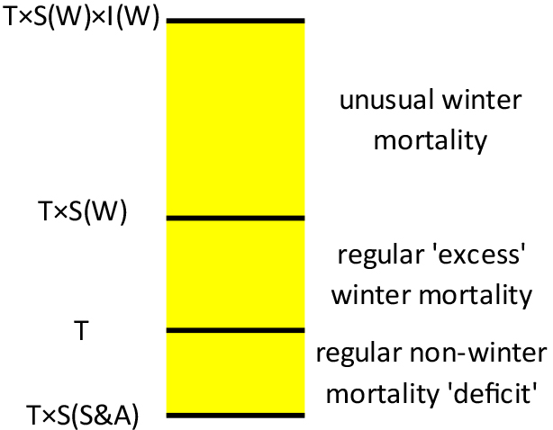
This now incorporates the seasonal fluctuation above the long-term average level of the series represented by the trend – in other words the amount that mortality is regularly higher in the winter periods, and the irregular – which contains an estimate of the part of the original series which is not the regular pattern, and which is therefore of primary interest in detecting unusual mortality events. These elements of the decomposed time series are shown diagrammatically in Fig. 4. Note that
Figure 4.
Diagrammatic representation of decomposition of the mortality time series into trend T, seasonal, S and irregular I components. (W) and (S&A) respectively refer to winter and combined spring and autumn components respectively. The descriptions show how the components relate to measures of winter mortality – see text for more details. There is an irregular term for the non-winter period too, but as the primary interest is in winter mortality, it is not included in the diagram.
We will define
2.2Properties of TEWM
TEWM has several advantages. It is minimally affected by unusual numbers of deaths in non-winter periods, as we illustrate more fully in Section 3, and therefore gives a more objective measure of excess winter deaths. It is based on a time series decomposition, which means that it is not necessary to wait for the comparator periods to become available as in the EWM measure, which cannot be calculated until the spring (Apr–July) period following the winter of interest has elapsed and its data have been processed. TEWM can be calculated as soon as March data have been collected and processed, and would therefore be available around four months earlier than EWM.
TEWM also has some disadvantages. Time series decomposition is achieved with the iterative application of complex moving averages, or using a model-based approach. Therefore, the values for the irregular, seasonal and trend elements are directly dependent on the filters or fitted model parameters used for the decomposition procedure. Importantly, this will lead to revisions in TEWM as new data points are added. Revisions in the existing EWM measure are minimal and occur only when provisional numbers are used for the most recent estimate.
Another issue that affects TEWM is whether any data points are identified as outliers; the standard approach to outliers in time series decomposition is to make a temporary prior-adjustment, where the outlier is replaced (wholly or partially) by an imputed value for the purposes of analysing the series, and then the prior adjustment is reversed in the output [29]. The identification of outliers can be subjective (based on prior knowledge about the series), or may be automated using a suitable algorithm. There are various methods for automatic identification of outliers, which may lead to different outcomes [31]. In addition, unusual data points at the beginning and end of a series cannot always be clearly classified as either an outlier or a level shift. This classification can have a big impact on the decomposition, because outliers are assigned to the irregular element, while level shifts are assigned to the trend-cycle [32].
3.Analysis of England and Wales deaths series
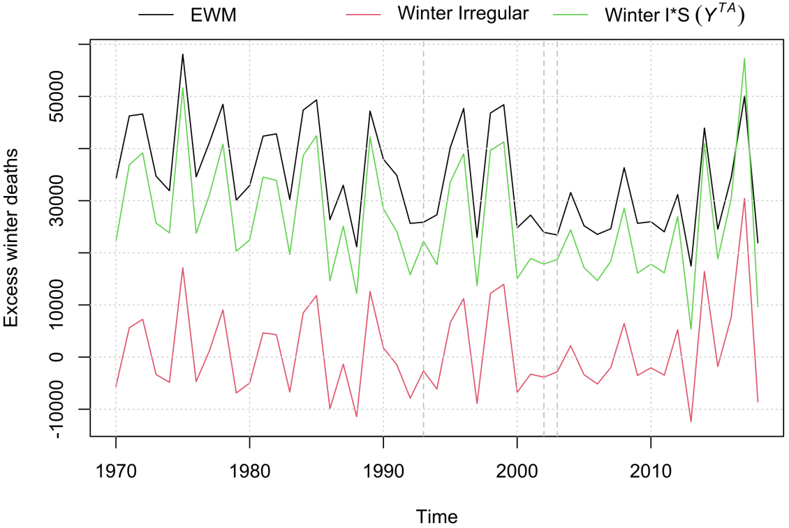
Figure 5.
Comparison of EWM (black/top line), EWM as measured by
3.1Method
Monthly time series of deaths in England and Wales spanning August 1970 to July 2019 were aggregated into four-month sections (quadrimesters) reflecting the
where
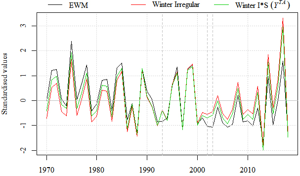
Figure 6.
Comparison of standardised values for EWM (black/darkest line), EWM as measured by
3.2Results
The current ONS method of calculating EWM is compared to the
Figure 7.
Top panel: Irregular terms from the time series decomposition, shown separately as series for winter, spring and autumn quadrimesters. Bottom panel: The irregular in the winter quadrimester and the mean irregular for the spring and autumn quadrimesters.
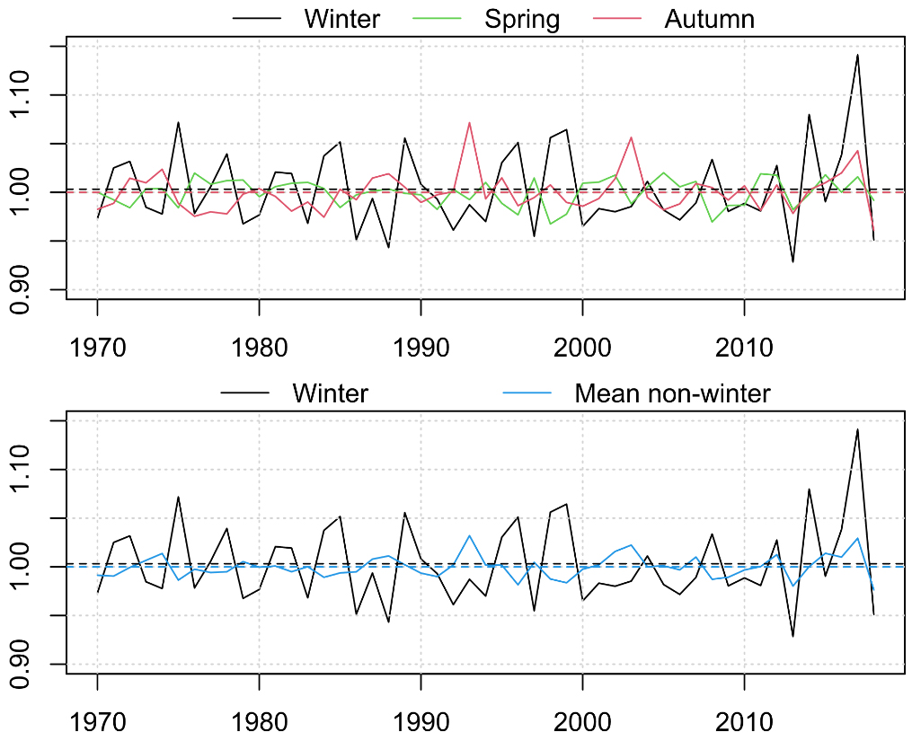
Figure 7 provides a comparison of the irregular elements for the winter period relative to spring and autumn (top panel), as well as relative to the average of the non-winter periods (i.e. the baseline used for estimating EWM, bottom panel).
The variance of unusual deaths is larger for winter periods. The top panel of Fig. 7 reveals instances of peaks of unusual deaths in the autumn period, sometimes higher than the corresponding winter period peaks (for example in 1993/94). It is these periods which cause the EWM measure to underestimate excess winter deaths and make it less suitable as a monitoring and analysis measure.
Figure 8.
Comparison of seasonal factors for winter months, spring (green/lightest line) and autumn (red/ darkest line) months, and the average of non-winter months. Dotted lines represent the mean value for the respective seasonal components.
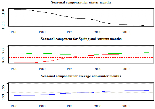
Although the general pattern of EWM and TEWM generally agree, as well as the differences caused by peaks in autumn deaths, there are differences in the evolution of the series. Specifically (see Fig. 6), EWM grows more slowly than TEWM. As expected, the estimated seasonal components for non-winter periods are notably lower than the winter period (Fig. 8, in line with the diagrammatic representation in Fig. 4). There is also a gradual reduction in the winter seasonal, reflecting a general decrease in the numbers of deaths occurring in winter, and an offsetting upward trend for the autumn seasonal factors. This shows a change in the balance of deaths between autumn and winter, while spring is largely unaffected. This induces the observed differences in the levels of EWM and TEWM.
Table 1
Revisions (percent) of estimated TEWM for the most recent four years of data. Each revision is as a percentage of the estimate in the previous publication year. Panel (a) shows the revisions when the outlier for winter (Dec-March) 2017 is identified only in 2018 and an outlier for winter 2014 is identified only in 2015. Panel (b) shows the reduced revisions when the outliers are identified by expert input as soon as they are available and forced permanently into the model (or at least until they are statistically significant, which is the case in this example)
| (a) | ||||
|---|---|---|---|---|
| Estimate for | Revision in publication year | |||
| winter | 2015–16 | 2016–17 | 2017–18 | 2018–19 |
| 2014–15 | 0.42% | 0.39% | ||
| 2015–16 | * | 1.08% | ||
| 2016–17 | * | 2.63% | ||
| 2017–18 | * | 5.96% | ||
| 2018–19 | * | |||
| (b) | ||||
| Estimate for | Revision in publication year | |||
| winter | 2015–16 | 2016–17 | 2017–18 | 2018–19 |
| 2014–15 | 0.42% | 0% | 0.27% | |
| 2015–16 | * | 0% | 0.58% | |
| 2016–17 | * | 1.41% | ||
| 2017–18 | * | 3.32% | ||
| 2018–19 | * | |||
3.3Revisions analysis
As described in Section 2.1, a potential limitation of TEWM is its susceptibility to revisions as new data points are added. A revisions history analysis (“revisions triangle”) of the last four years of data was undertaken (Table 1, see also supplementary material), examining the revision as a percentage of the previous estimate for that reference period as more data become available. The ARIMA model was held constant, and the analysis was performed with each successive March being the last available datapoint, providing a complete winter period. The automatic detection for outliers (one-off unusual values) implemented in TRAMO-SEATS was used as an illustration. One of the limitations of using automatic outlier detection for the regression part of the ARIMA model is that what is estimated to be an outlier may change from one year to the next. In a more formal production setting, outliers should be judged with expert knowledge, not entirely depending on automatic detection procedures. Also, it is likely that when an outlier is modelled based on prior knowledge, it would be kept in the model as new data is added. This will reduce the size of future revisions. For the current purposes, the assumption of no prior knowledge and use only of the automatic outlier detection was compared to revisions when an outlier is identified sooner and kept in the model.
Figure 9.
Estimated TEWM series as it evolves from first publication in 2002-3, using automatic outlier detection. Each shade represents a different vintage of the series, and where they overlie each other revisions are minimal.
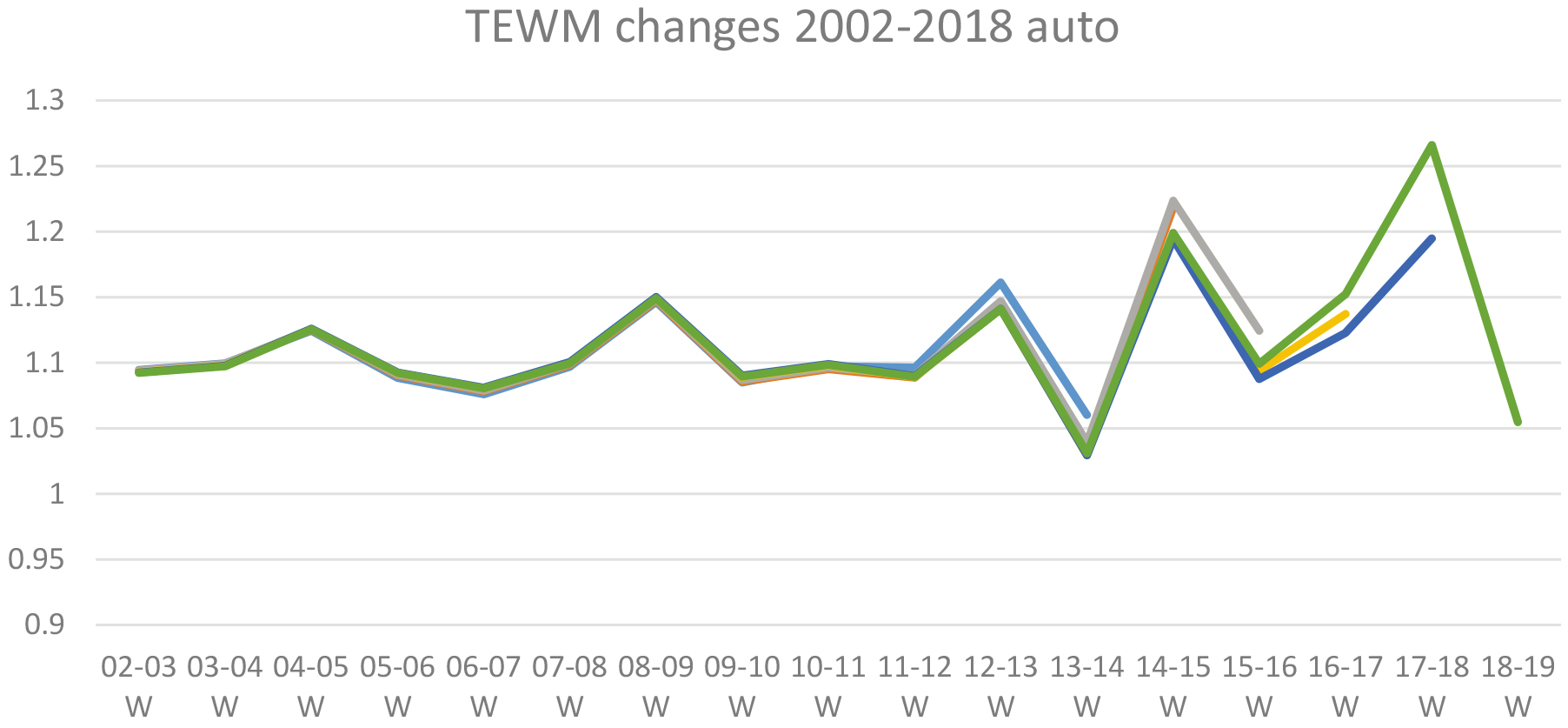
To illustrate the impact of “unstable” outliers, in Table 1(a), for publication year 2015–16, winter 2014–15 was estimated to be an outlier value as it was unusually high for the local values at the time. However, as more data became available, it was no longer considered an outlier. As a result, the analysis suggests that when 2016–17 data became available, TEWM for period 2015–16 was revised down by 2.73% and the TEWM for the previously outliered value of 2014–15 dropped by 2.14%. Furthermore, in publication year 2018–19 (the latest used in this analysis), the winter period 2017–18 was estimated to be an outlier value, but this was not the case when winter 2017–18 was the latest period. Modelling winter 2017–18 as an outlier led to an overall 5.96% upward revision of TEWM with the latest data, and also revised previous periods’ estimates upwards. It is generally expected that revisions would be greatest for the latest data points, as the table illustrates (see also the full revisions history in the supplementary material: Revisions_tables_autoAO.xlsx). Identifying an outlier adjusts the decomposition so that the seasonal (what is considered as typical for the series) is decreased in favour of the irregular component. In this case the irregular goes up substantially, as the 2017–18 winter was higher than usual. In comparison, the revisions for winter 2017–18 are lower if it is modelled as an outlier as soon as that data point becomes available (rather than a year later), and it is kept as an outlier in the model in the next publication year (denoted by 2017–18
Figure 9 shows a “porcupine plot” of the successive estimates of TEWM as time progresses from 2002–3. It is clear that the model is stable in the earlier years of this plot, but that there is more volatility in the most recent years. Nevertheless, the revisions are small. The average revision one year after first publication (which is expected to be the largest because the model can be affected more by the addition of new data points) is 0.97% for the 89–90 to 17–18 estimates of TEWM, and 2.60% in the last four years (14–15 to 17–18).
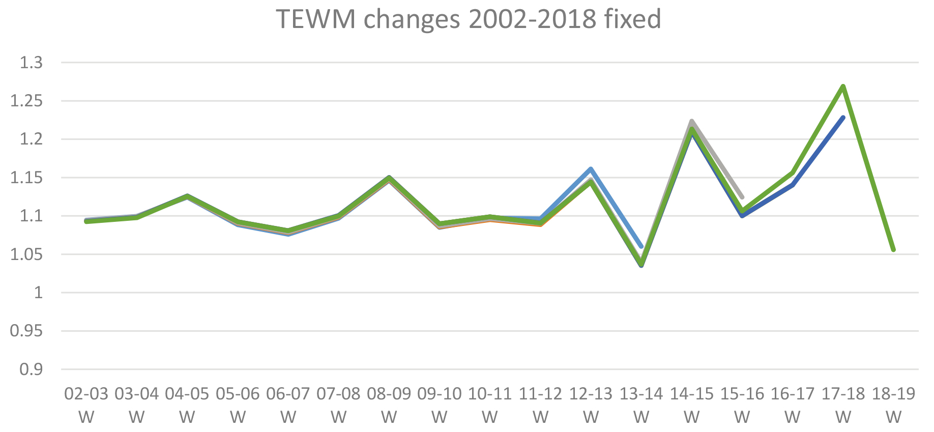
In comparison, Fig. 10 illustrates the same data but with stable outliers in the model (corresponding to Table 1(b)). The differences between the vintages are visibly smaller, and the revision one year after first publication for the period 89–90 to 17–18 is 0.81% and for the last 4 years it is 1.48%.
Figure 10.
Estimated TEWM series as it evolves from first publication in 2002–3, with fixed outliers for winter 2014 and 2017. Each shade represents a different vintage of the series, and where they overlie each other revisions are minimal.
4.Discussion
A time series decomposition approach to defining an official statistic to measure the excess of deaths in a winter period, TEWM, has several advantages. It is much better aligned with the intuitive interpretation of “excess winter mortality”, and is relatively unaffected by large numbers of deaths in non-winter periods – which only contribute inasmuch as they affect the time series model and its fit. This would in particular be seen in 2020 and possibly 2021 where coronavirus would cause an extreme spike in spring period mortality (not included in this analysis). TEWM also provides a measure which is much more timely than the current EWM as it can be estimated as soon as the winter reference period is available. By contrast, EWM calculations cannot be performed until June data is available.
The different time series components (trend-cycle, seasonal and irregular) can be provided, and interpreted by technically competent users to provide better information than from the rather crude moving average of the existing EWM measure. Regardless of the frequency of observations, it can be very useful to isolate specific aspects of interest in addressing an underlying research question. For example, the irregular component provides an ‘uncontaminated’ measure of excess deaths during winter, while the seasonal element for the winter period shows changes in trends in winter mortality and how seasonality evolves over the years in non-winter periods as well. As the seasonal adjustment uses a model-based method it is also possible to derive confidence intervals for these components. A comparison of the current and potential outputs for publication is shown in Fig. 11.
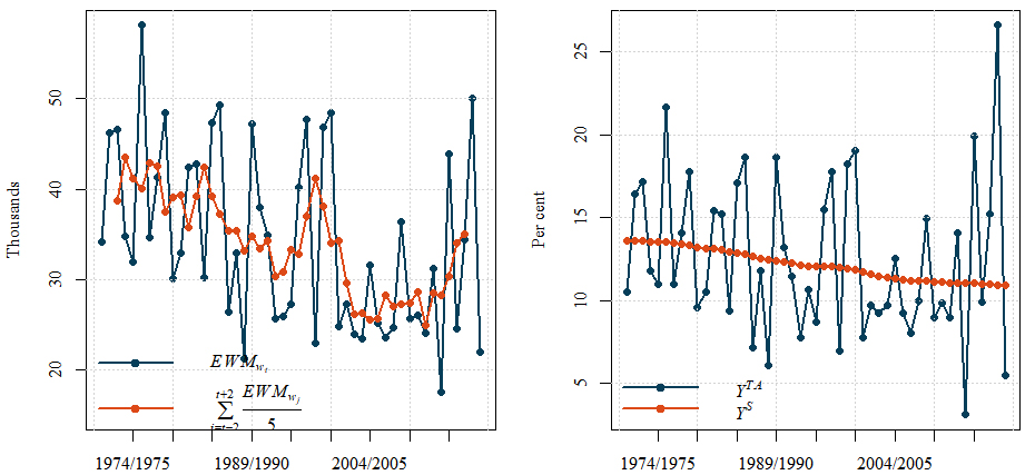
Figure 11.
Excess winter deaths for England and Wales and trend in excess winter deaths. Left: current method for number of excess winter deaths together with a five-point moving average. Right: proposed method for TEWM as per cent of all winter deaths, with the winter seasonal component
As always there is a price to pay for such an improvement, and in this case it is the revisions to the new series as the time series model evolves when new observations are added. The use of prior adjustments and ARIMA model selection can also generate revisions in the final estimates. However, revisions are part of the standard seasonal adjustment process and the aim is always to keep them as small as possible. The impact of revisions on the statistics, as shown in Table 1, is small, so it is likely that analytical conclusions will be only minimally affected by such revisions. These issues can be minimised or avoided if the best model is identified and then fixed for a period, with regular checking to ensure that it remains appropriate. The proposed method addresses some of the limitations of the current measure of excess winter mortality, also identified by other authors [5], using a seasonal adjustment method which is well supported and practiced widely in official statistics. The new statistic is also better aligned conceptually with the name of the statistic - it does measure the excess of deaths during the winter period compared with the long-run average of the series, rather than compared with some more arbitrarily-defined baseline. Nevertheless, should such a series be introduced it would probably be wise to give it a different name to distinguish it from the long-established statistic which is already produced.
Notes
1 We use the TRAMO-SEATS seasonal adjustment functionality of JDemetra+ version 2.2.2 to fit all the time series models presented here. This is software for seasonal adjustment and time series modelling developed by the National Bank of Belgium in cooperation with the Deutsche Bundesbank and Eurostat. It is freely available for download from https://github.com/jdemetra/jdemetra-app/releases/tag/v2.2.2; more details in Appendix 1. All remaining manipulation of data and results was undertaken with RStudio Desktop version with R version 3.4.4. The processing was undertaken on an Intel Core i5 vPro Lenovo laptop running at 2.40 GHz with 8 GB RAM running the Windows 10 Operating System.
Acknowledgments
The views in this paper are those of the authors and do not necessarily represent the views of their respective organisations.
References
[1] | Bull GM, Morton J. Environment, temperature and death rates. Age and Ageing. (1978) ; 7: (4): 210-224. doi: 10.1093/ageing/7.4.210. |
[2] | Laake K, Sverre J. Winter excess mortality: a comparison between Norway and England plus Wales. Age and Ageing. (1996) ; 25: (5): 343-348. doi: 10.1093/ageing/25.5.343. |
[3] | Winter H, Tawn J. Modelling heatwaves in central France: A case study in extremal dependence. Journal of the Royal Statistical Society: Series C (Applied Statistics). (2016) ; 65: (3): 345-365. doi: 10.1111/rssc.12121. |
[4] | Lawlor D, Harvey D, Dews H. Investigation of the association between excess winter mortality and socio-economic deprivation. Journal of Public Health. (2000) ; 22: (2): 176-181. doi: 10.1093/pubmed/22.2.176. |
[5] | Hajat S, Gasparrini A. The excess winter deaths measure: Why its use is misleading for public health understanding of cold-related health impacts. Epidemiology. (2016) ; 27: (4): 486-491. doi: 10.1097/EDE.0000000000000479. |
[6] | Gasparrini A, Guo Y, Hashizume M, Kinney P, Petkova E, Lavigne E, Zanobetti A, Schwartz J, Tobias A, Leone M, Tong S, Honda Y, Kim H, Armstrong B. Temporal variation in heat-mortality associations: A multicountry study. Environmental Health Perspectives. (2015) a; 123: (11): 1200-1207. doi: 10.1289/ehp.1409070. |
[7] | Huynen M, Martens P, Schram D, Weijenberg M, Kunst A. The impact of heat waves and cold spells on mortality rates in the Dutch population. Environmental Health Perspectives. (2001) ; 109: (5): 463-470. doi: 10.1289/ehp.01109463. |
[8] | Gasparrini A, Guo Y, Hashizume M, Lavigne E, Zanobetti A, Schwartz J, Tobias A, Tong S, Rocklov J, Forsberg B, Leone M, De Sario M, Bel M, Guo YL, Wu C, Kan H, Yi S, Coelho M, Saldiva P, Honda Y, Kim H, Armstrong B. Mortality risk attributable to high and low ambient temperature: a multicountry observational study. The Lancet. (2015) b; 386: (9991): 369-375. doi: 10.1016/S0140-6736(14)62114-0. |
[9] | Office for National Statistics. Excess deaths in your neighbourhood during the coronavirus (COVID-19) pandemic, available from https://www.ons.gov.uk/peoplepopulationandcommunity/birthsdeathsandmarriages/deaths/articles/excessdeathsinyourneighbourhoodduringthecoronaviruscovid19pandemic/2021-08-03. (accessed 12/9/2021). |
[10] | Johnson H, Griffiths C. Estimating excess winter mortality in England and Wales. Health Statistics Quarterly/Office for National Statistics. (2003) ; 20: : 19-24. |
[11] | World Health Organization(WHO). Health impact of low indoor temperatures: Report on a WHO meeting. Copenhagen: WHO Regional Office for Europe, (1987) . |
[12] | World Health Organization (WHO). Housing, energy and thermal comfort: A review of 10 countries within the WHO European region.Copenhagen: WHO Regional Office for Europe. (2007) ; Available from http//www.euro.who.int/__data/assets/pdf_file/0008/97091/E89887.pdf: (accessed 19/04/2020). |
[13] | Eurostat. Deaths (total) by month. (2020) ; http//appsso.eurostat.ec.europa.eu/nui/show.do?query=BOOKMARK_DS-061474_QID_-DFCB8EB_UID_-3F171EB0&layout=MONTH,L,X,0;GEO,L,Y,0;UNIT,L,Z,0;TIME,C,Z,1;INDICATORS,C,Z,2;&zSelection=DS-061474TIME,2015;DS-061474UNIT,NR;DS-061474INDICATORS,OBS_FLAG;&rankName1=UNIT_1_2_-1_2&rankName2=INDICATORS_1_2_-1_2&rankName3=TIME_1_0_1_0&rankName4=MONTH_1_2_0_0&rankName5=GEO_1_2_0_1&rStp=&cStp=&rDCh=&cDCh=&rDM=true&cDM=true&footnes=false&empty=false&wai=false&time_mode=ROLLING&time_most_recent=false&lang=EN&cfo=%23%23%23%2C%23%23%23.%23%23%23: (accessed 30/07/2020). |
[14] | Fischer EM, Schär C. Consistent geographical patterns of changes in high-impact European heatwaves. Nature Geoscience. (2010) ; 3: : 398-403. |
[15] | Fowler T, Southgate R, Waite T, Harrell R, Kovats S, Bone A, Doyle Y, Murray V. Excess winter deaths in Europe: a multi-country descriptive analysis. European Journal of Public Health. (2015) ; 25: (2): 339-345. doi: 10.1093/eurpub/cku073. |
[16] | Pascal M, Wagner V, Le Tertre A, Laaidi K, Honore C, Benichou F, Beaudeau P. Definition of temperature thresholds: the example of the French heat wave warning system. International Journal of Biometeorology. (2013) ; 57: (1): 345-365. doi: 10.1007/s00484-012-0530-1. |
[17] | Gasparrini A, Guo Y, Hashizume M, Lavigne E, Tobias A, Zanobetti A, Schwartz J, Leone M, Michelozzi P, Kan H, Tong S, Honda Y, Kim H, Armstrong B. Changes in susceptibility to heat during the summer: A multicountry analysis. American Journal of Epidemiology. (2016) ; 183: (11): 1027-1036. doi: 10.1093/aje/kwv260. |
[18] | Pattenden S, Nikiforov B, Armstrong B. Mortality and temperature in Sofia and London. Journal of Epidemiology & Community Health. (2003) ; 57: (8): 628-633. doi: 10.1136/jech.57.8.628. |
[19] | Revich B, Shaposhnikov D. Excess mortality during heat waves and cold spells in Moscow, Russia. Occupational and Environmental Medicine. (2008) ; 65: (10): 691-696. doi: 10.1136/oem.2007.033944. |
[20] | Vicedo-Cabrera A, Forsberg B, Tobias A, Zanobetti A, Schwartz J, Armstrong B, Gasparrini A. Associations of inter- and intraday temperature change with mortality. American Journal of Epidemiology. (2016) ; 183: (4): 286-293. doi: 10.1093/aje/kwv205. |
[21] | Office for National Statistics, UK (ONS) Excess winter mortality in England and Wales: 2018 to 2019 (provisional) and 2017 to 2018 (final). 2019. Available from https://www.ons.gov.uk/peoplepopulationandcommunity/birthsdeathsandmarriages/deaths/bulletins/excesswintermortalityinenglandandwales/2018to2019provisionaland2017to2018final. (accessed 20/4/2020). |
[22] | National Records of Scotland. Winter Mortality in Scotland 2018/19. 2019, Available from https//www.nrscotland.gov.uk/files//statistics/winter-mortality/2019/winter-mortality-18-19-pub.pdf: (accessed 01/05/2020). |
[23] | Northern Ireland Statistics and Research Agency (NISRA). Tables for Excess Winter Mortality 2017/18. 2018. Available from https//www.nisra.gov.uk/sites/nisra.gov.uk/files/publications/EWM_2017_18_WEB.xls: (accessed 01/05/2020). |
[24] | Curwen M. Excess winter mortality: a British phenomenon? Health Trends. (1990) ; 22: : 169-175. |
[25] | Healy J. Excess winter mortality in Europe: a cross country analysis identifying key risk factors. Journal of Epidemiology and Community Health. (2003) ; 57: (10): 784-789. doi: 10.1136/jech.57.10.784. |
[26] | Carson C, Hajat S, Armstrong B, Wilkinson P. Declining vulnerability to temperature-related mortality in London over the 20th century. American Journal of Epidemiology. (2006) ; 164: (1): 77-84. doi: 10.1093/aje/kwj147. |
[27] | Hales S, Blakely T, Foster RH, Baker M, Howden-Chapman P. Seasonal patterns of mortality in relation to social factors. Journal of Epidemiology & Community Health. (2002) ; 66: (4): 379-384. doi: 10.1136/jech.2010.111864. |
[28] | Chatfield C. The analysis of time series: An introduction. 6th ed. CRC Press: Boca Raton, Florida, (2003) . |
[29] | Ladiray D, Quenneville B. Seasonal adjustment with the X-11 method. Lecture Notes in Statistics 158; Springer, (2001) . |
[30] | Gomez V, Maravall A. Programs TRAMO and SEATS: Instructions for the user. Banco de España – Servicio de Estudios, DT 9628. (1997) . |
[31] | Eurostat. ESS guidelines on seasonal adjustment, Luxembourg: Publications Office of the European Union. (2015) ; doi: 10.2785/317290. |
[32] | United States Census Bureau. X-13ARIMA-SEATS Reference Manual. (2017) ; available from https//www.census.gov/ts/x13as/docX13AS.pdf: (accessed 30/07/2020). |
Appendices
Appendix 1
JDemetra+ version 2.2.2 is software for seasonal adjustment and time series modelling developed by the National Bank of Belgium in cooperation with the Deutsche Bundesbank and Eurostat. It incorporates X-12 which is the standard non-parametric approach to seasonal adjustment based on moving average filters [29, 32] and TRAMO-SEATS which is an implementation of ARIMA modelling designed for use in official statistics [30]. See https://ec.europa.eu/eurostat/cros/content/software-jdemetra_en for more details. One of its key advantages is the availability of both approaches, which can therefore be freely used and compared within the same framework. It is freely available for download from https://github.com/jdemetra/jdemetra-app/releases/tag/v2.2.2, and requires Java SE 8 or higher.


