
Sequence-based malware detection using a single-bidirectional graph embedding and multi-task learning framework
Abstract
As an important part of malware detection and classification, sequence-based analysis can be integrated into dynamic detection system for real-time detection. This work presents a novel learning method for malware detection models that leverages advances in graph embedding for fusing the n-gram data into a one-hot feature space with different transmission directions. By capturing the information flow, our method finds a better feature representation for detection tasks with rely solely on sequence information. To enhance the stability of feature representation, this work adopts a multi-task learning strategy which achieves better performance in independent testing. We evaluate our method on two different realworld datasets and compare it against four superior malware detection models. During malware detection using our method, we conducted in-depth discussions on feature length, graph embedding direction, model depth, and different multi-task learning strategies. Experimental and discussion results show that our method significantly outperforms alternative approaches across evaluation settings.
1.Introduction
With the rapid development of computer and internet technology, malicious software (Malware) has continued to impact cyberspace security. In recent years, due to its large profit, the scale, categories, and qualities of malware have grown considerably. According to a report from AV-TEST,11 mass malware attacks and threats to the internet reached a new peak. Therefore, it is necessary to develop technology for rapid malware identification.
Recently, due to the increasing number of available malicious code, machine learning methods for malware detection have been employed. Malware detectors based on signature databases [11] or static analysis [32] are facing increasing difficulty in separating malicious pieces from legitimate code because of the development of malware obfuscation and variant technology. To address this issue, multiple studies on malware identification based on traditional machine learning methods have been carried out. For example, Mirza et al. [28] used a support vector machine decision tree, and boosting on decision tree to classify malware families. Moser et al. [26] proposed a feature extraction method based on gray-scale images and applied the shared nearest neighbor (SNN) to detect malware.
In the last five years, researchers have leveraged deep learning (DL) methods to distinguish malware. For example, Ding and Zhu [43] used opcode sequences to identify malware. Vinayakumar et al. [37] successfully provided a novel image processing technique for malware classification using raw byte sequences from binary files. Compared to traditional machine learning techniques, DL has the advantage of reducing the work of representing malware in digital arrays and can generate useable features during training epochs [21]. To a certain extent, detection methods based on deep learning techniques are the core direction of current malicious code research.
For existing features, such as file header information [24] and byte sequences [27], feature extraction is difficult and the extracted features cannot be utilized effectively for malware classification. Consequently, many researchers have focused on feature engineering [31,35]. In static detection, binary files are typically used as the source for malware sample characterization. After disassembling a binary file, the disassembled result will be used as the input to the model. In a recent study [25], researchers used static analysis and Nonnegative Matrix Factorization to detect metamorphic malware, which can evade traditional signature-based detection methods. Kumar et al. [22] have proposed a machine learning-based solution to improve the efficiency of malware detection. Their approach involves creating an integrated feature set that combines the portable executable header fields with various machine learning algorithms.
Dynamic behavior analysis techniques are a popular approach for extracting features from programs for malware detection. These techniques capture the behavioral characteristics of malware, including file system activity, registry activity, and network activity. Some studies even use machine activities, such as energy consumption metrics [9], to detect malware. Ahmed et al. [1] proposed a non-signature-based detection approach based on the effective Windows API call sequences, using supervised machine learning techniques. Machine learning algorithms based on decision trees can then be adopted to classify malware [14]. Kim et al. [19] proposed a malware detection and classification system based on dynamic analysis using the behavioral sequence of malware (API call sequence) and sequence alignment algorithm (MSA). Their approach analyzing the behavioral sequence of the malware and comparing it with a reference sequence using MSA. Hwang et al. [16] proposed a two-stage mixed ransomware detection model that incorporates both a Markov model and a Random Forest machine learning model. Their approach focuses on the Windows API call sequence pattern to capture the characteristics of ransomware and uses the Random Forest model to control both false positive and false negative error rates. Other studies have also utilized CNN [33] or LSTM [13] layers to construct models that use API call sequences as features.
Some studies combine static analysis techniques to extract features of malware with dynamic analysis techniques to capture the behavioral characteristics of malware, and then use machine learning algorithms to classify malware [34]. Ndibanje et al. [29] proposed a method to de-obfuscate and unpack malware samples, and used cross-method-based big data analysis to dynamically and statistically extract features from malware. Their approach relies on Application Programming Interface (API) call sequences to detect behavior such as network traffic, file modification, registry value modification, and process creation. Huang et al. [15] proposed a two-stage mixed ransomware detection model that combines a Markov model and a Random Forest machine learning model. Their approach focuses on the Windows API call sequence pattern to capture the characteristics of ransomware and uses the Random Forest model to control both false positive and false negative error rates.
We have noticed that there has been a lack of research that uses API call sequences as features, and the temporal characteristics of API call sequences have not been fully utilized in previous studies. Our research aims to make a small yet significant contribution to the field of malware family classification by presenting a novel model based on the API call sequence. The following two key techniques were used. (1) To improve the characterization using the API call sequence, we used graph embedding as a representation of the sequence. Using graph embedding can fuse the context of the API call sequence globally without additional information. (2) To enhance the prediction ability from the represented sequences, we adopted a multitask learning strategy to make full use of latent information and achieve a better optimization mechanism.
In practice, first, we preprocessed the obtained API call sequence involved in the execution of malware samples. Then, we optimized the structure of the neural network architecture by adjusting the feature length, the number of LSTM network layers, the location of the convolutional layers, and the direction of the graph embedding information flow. Finally, we used multitask learning [18] to optimize the prediction performance. The results showed that the proposed method outperforms other methods on the same datasets. The code for this research has been made available on GitHub.22
Our contributions are as follows:
– A single-bidirectional graph embedding framework was introduced for malware detection based on API call sequences, bringing considerable high efficiency and accuracy.
– Different multitask learning strategies were used for malware detection, and the differences in the prediction performance were compared and discussed.
– Many hyperparameter optimization operations of the neural network architecture were processed and discussed separately, and the impact on the prediction performance was recorded and discussed
2.Research methodology
2.1.Overview
In this section, we will provide an introduction to the fundamental concepts and implementation process of graph embedding. We will also discuss the essential components of our detection model, including the multitask learning strategy and the bidirectional long short term memory (LSTM) recurrent neural network module.
2.2.Primer on graph embedding
Graph-based data is inherently unstructured, unlike images that are neatly arranged in matrix forms. To overcome this challenge, graph convolutional network can automatically learn discriminative latent features from graphbased data [20]. In a graph
To perform the normalization operation on
Let X denote the features of the nodes on graph G, where
The graph convolution operation defined by Equation (3) aggregates local substructure information by considering the nodes’ immediate neighborhoods. Building upon Equation (3), we proposed a graph embedding method that learns the transmission direction of the information flow within the sequence information. Let
Fig. 1.
Flow chart of our method.
In summary, the graph embedding method comprehensively considers both the propagation and reception of node information flow, which enables the full utilization of latent information from a single data feature.
2.3.The overall process of our method
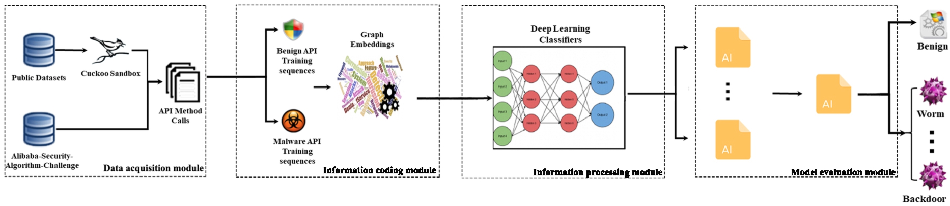
This section outlines the main technical route of our method, which is shown in Fig. 1. The method mainly consists of four modules:
A. Data acquisition module: This module obtains the API call sequence by executing the malware executable file in the dataset within a Cuckoo sandbox. The API call sequence obtained from the Cuckoo sandbox is serialized.
B. Information encoding module: This module generates a behavior graph according to the API call sequence and API call set. The behavior graph is then embedded using graph embedding techniques.
C. Information processing module: This module processes the embedded information using a Bi-LSTM network and an attention mechanism.
D. Model evaluation module: This module evaluates the model by calculating cross-entropy and other indicators.
2.3.1.Generation of a behavior graph
After processing the time series of API calls involved in the malware dataset, a behavior graph is generated. The behavior graph is a graphical representation of the malware in the attack behavior of the target host. Algorithm 1 is used to generate the behavior graph, which combines time (API call time series) and spatial information (adjacency and connectivity) in the behavior graph. By using the behavior graph as input to graph convolution, effective features of the data can be more effectively and comprehensively extracted, resulting in improved accuracy of malware detection.
Algorithm 1:
The generation of a behavior graph
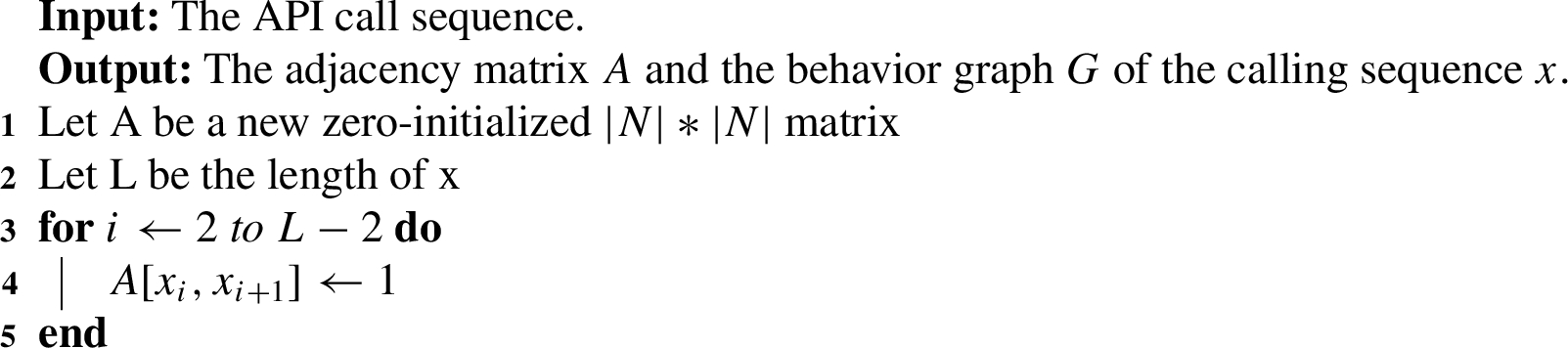
Fig. 2.
Operating principal diagram of our method (propagation direction).
2.3.2.Directional graph embedding module
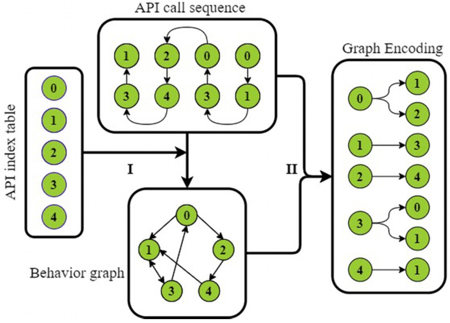
An example is provided to illustrate the use of single-bidirectional graph embedding module. Software API calls have a strong logical connection to each other, and the information flow provided by the graph embedding method can more naturally reflect the behavior of the software. As shown in Fig. 2 and Fig. 3, the API index table represents all the API types involved in the malware attack process, and the API call sequence represents the entire time sequence of malware sample’s execution. The involved API index table, denoted as
Fig. 3.
Operating principal diagram of our method (receiving direction).
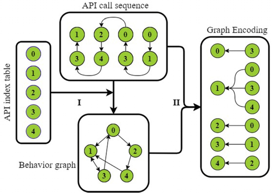
As shown in Fig. 2 and Fig. 3, step is the graph embedding process. In the graph embedding process, we used matrix multiplication to generate the connection environment of every API call. Different ways of using matrix multiplication can generate environment representations in different directions of information flow. This step has been overlooked by previous researchers. By comprehensively considering both the propagation and reception of node information flow in the behavior graph, we can more effectively and comprehensively extract features.
The step of Fig. 2 can be represented by formula
Since the proposed graph embedding method can encode sequential data in two directions, we provided two models as a comparison to explore the relationship between the direction of encoding and the prediction performance. These two models have the same structure as our method but use different training data. The models were named ‘single graph embedding-Next model’(SGENext) and ‘single graph embedding-Pre model’(SGEPre). SGENext represents a model that uses only graph encoding that uses the direction to the last step,
2.4.The structure of built models
After extracting features from the malware sequences, we used several neural network layers for information processing and prediction. Similar to other research, we employed the LSTM and CNN layers to generate the features for final rediction. We also used a multi-task learning strategy for loss computation. We tested multiple models using different combinations of the layers, and the details are provided in Section 4. Below is a brief introduction of the layers and multi-task learning strategy.
2.4.1.Convolutional neural network module
The formulation of the convolution operation is as follows:
2.4.2.Bidirectional long short-term memory recurrent neural network module
A long short-term memory (LSTM) network is a type of recurrent neural network (RNN) [10]. LSTM networks retain the advantages of an RNN for processing time series data by combining current calculations with historical input information and improving the memorization mechanism by integrating both short-term memory and long-term memory. To some extent, LSTMs solve the challenge of an RNNs only memorizing short-term historical input information and not effectively solving problems that require long-term memory.
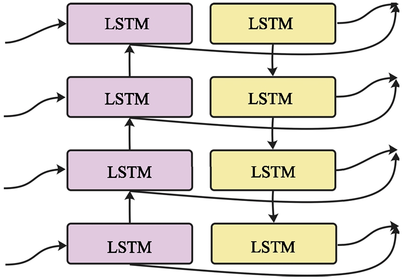
However, because an LSTM network can process data only in a sequential sequence, when processing the API sequence, only single-direction graph embedding information can be obtained and the other direction information is lost. In other words, there is a two-way response dependency, and a traditional LSTM model cannot encode information from back to front. To address this issue, a Bi-LSTM model is used, which combines a forward LSTM with a reverse LSTM (as illustrated in Fig. 4), improving the LSTM network and forming a two-way RNN model.
Fig. 4.
Bi-LSTM schematic diagram.
2.4.3.Attention mechanism module
In the serialization features we extracted, each portion of the behavior sequence contributes differently to the final classification result. To determine which parts play the most important role, we constructed a weight distribution mechanism for serialized features. An effective solution is to use an attention mechanism, which can learn information across the sequence by computing the similarity between normalized queries and keys, and then assign sequence information based on the generated similarities. In our study, the attention layers were added after the LSTM layers for the information rearrangement.
2.4.4.Multi-task learning strategy
Compared to single-tasking learning, multitasking learning can avoid repeatedly calculating features in shared layers and has the potential to improve performance if the associated tasks share complementary information. In our study, we applied multitasking learning to malware detection and family classification, as we believe these tasks are related. The goal of multi-task learning is to improve learning efficiency and prediction accuracy by learning multiple objectives from a shared representation [6,36]. To implement multi-task learning, we designed different loss values. We used two different multi-task learning strategies: (1) We used a categorical cross entropy loss for identifying all eight classes and eight binary cross entropy losses for identifying a certain class of malware code. (2) We used a categorical cross entropy loss for all eight classes and 28 binary cross entropy losses for all malware code class pairs (i.e.,
3.Experiments and results
In this section, we describe the experimental datasets and evaluate the effectiveness of our model on the malware detection task by 5-fold cross validation. The training/testing set proportion was set to 4:1. In addition to the methods provided in this work, we also collected other works that used API call sequences as input for prediction to compare both malware detection and classification performance.
3.1.Datasets
Since malware is constantly being updated, the majority of new malware samples are polymorphic variants of known malware [4]. Therefore, we followed the approach of Ding et al. [8] and classified malware samples with similar malicious behaviors into the same family.
To facilitate comparison, we evaluate our method on two different real-world datasets: the Tianchi dataset and the dataset from Catak’s work. The latter was collected using the git command-line utility from various malware samples projects on Github, while the tianchi dataset was obtained from the Alibaba–Security–Algorithm–Challenge33 to test our method. In the dataset used in Catak’s work, each data is an API call sequence, where each element is an integer representing a specific Windows API call. These sequences can be used to represent the behavior of malicious software, such as file operations, process creation, registry modifications, and so on. In contrast, the tianchi dataset is an API instruction sequence extracted from a sandbox simulation of Windows executable programs. Each data point contains five fields, including file ID, file label, API name called by the file, thread ID that made the API call, and order number of the API call in the thread. All executable programs were desensitized, and there were a total of eight category labels, including Normal, Infectious viruses, Trojan horse programs, Mining programs, DDOS Trojan horses, Ransomware, Backdoor programs, and Worms.
The data preprocessing stage includes four concepts.
(1) According to Kolosnjaji’s [21] work, nonconsecutive repeated API calls were considered to avoid tracking loops.
(2) Considering the complexity of the data, only sequences from the parent process were extracted.
(3) We built a list of unique API calls, considering all the samples. Each API call name was then converted to a unique integer identifier, which was equal to the index of the API call name in the list.
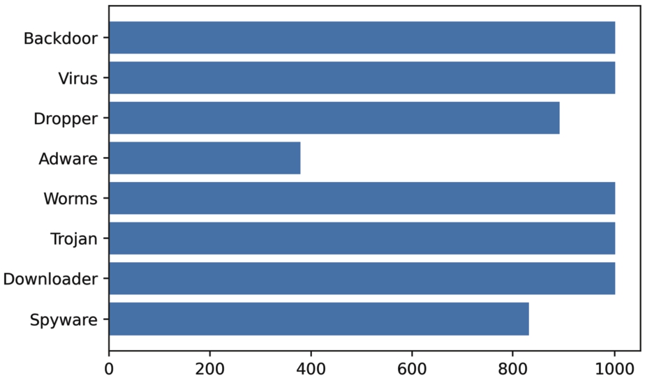
(4) The Tianchi dataset used in our study exhibited an unbalanced distribution of samples, as illustrated in Fig. 5. To mitigate the effect of class imbalance during training, we employed the SMOTE [38] method to generate synthetic samples from the existing ones, resulting in a balanced dataset with a total of 26,824 samples (referred to as the Balanced Tianchi dataset). This approach aimed to address the issue of imbalanced datasets by generating synthetic minority samples between existing samples and their neighbors. By increasing the representation of the minority class, the model is better able to learn from it, ultimately enhancing its predictive performance. In contrast, the malware analysis dataset used in Catak’s work [7] comprised 7,107 malware samples from different classes, as depicted in Fig. 6
Fig. 5.
Distribution of sample categories in tianchi dataset.
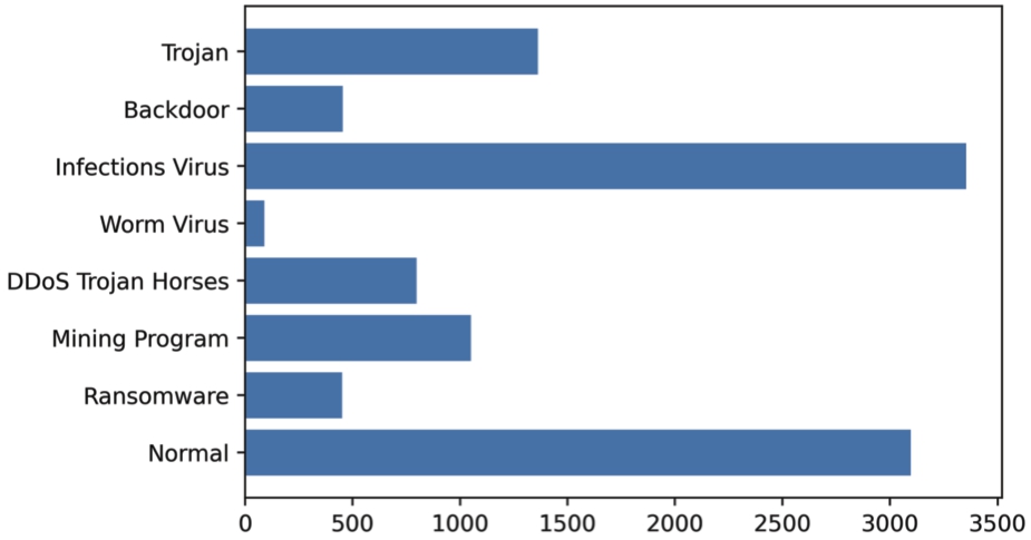
Fig. 6.
Distribution of sample categories in dataset from catak’s work.
3.2.Evaluation metrics
Like other works on classification problems, this study uses the evaluation metrics listed in Table 1 to assess the performance of the model.
Table 1
Evaluation metrics
| Eq | Metric | Formula | Detail |
| 1 | Accuracy | The classification accuracy score is the percentage of all categories that are correct | |
| 2 | Precision | The ratio of the number of correctly identified malware samples to the total number of identified samples. | |
| 3 | Recall | The ratio of the number of correctly identified malware samples to the number of samples that should be identified. | |
| 4 | F1-Score | The F1-score is an indicator used in statistics to measure the accuracy of the model. At the same time, the accuracy and recall rate of the classification model are considered. |
3.3.Comparison with existing methods
The purpose of this section is to benchmark the efficiency of the proposed method with existing relevant approaches. we divide the work into two steps.
Table 2
Comparison of detection results (original tianchi dataset)
| Metric/model | Our method | LSTM | RF | SGENext | SGEPre | Oliverira et al. [30] |
| Precision | 0.9775 | 0.9499 | 0.9148 | 0.9441 | 0.9492 | 0.9425 |
| Recall | 0.9622 | 0.9518 | 0.9490 | 0.9544 | 0.9585 | 0.9551 |
| Accuracy | 0.9467 | 0.9223 | 0.9077 | 0.9276 | 0.9374 | 0.9268 |
| F1-Score | 0.9698 | 0.9508 | 0.9316 | 0.9492 | 0.9538 | 0.9390 |
Step 1: Rapid detect malware from all samples
In Table 2, we compare the performance of our model with five other methods on the tianchi dataset: a LSTM, SGENext, SGEPre, a random forest (RF) and the methods proposed by Oliverira et al. [30]. In our experiment, the LSTM-based method reaches a 92.23% accuracy rate, 95.08% F1-score, 95.18% recall and 94.99% precision rate. Meanwhile, the RF-based method reaches a 90.77% accuracy rate, 93.16% F1-score, 94.9% recall and 91.48% precision rate. Our method outperformed these four methods in all metrics, as shown in the confusion matrix in Fig. 7.
Fig. 7.
Confusion matrix of malware detection.
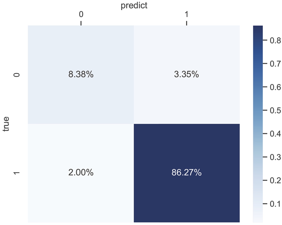
Table 3
Comparison of detection results (balanced tianchi dataset)
| Metric/model | Our method | LSTM | RF | SGENext | SGEPre | Oliverira et al. [30] |
| Precision | 0.9561 | 0.9307 | 0.9396 | 0.9358 | 0.9428 | 0.9495 |
| Recall | 0.952 | 0.9398 | 0.9297 | 0.9057 | 0.9293 | 0.9519 |
| Accuracy | 0.9457 | 0.9391 | 0.9348 | 0.9215 | 0.9387 | 0.9277 |
| F1-Score | 0.9535 | 0.9352 | 0.9346 | 0.9205 | 0.936 | 0.9507 |
In Table 3, we compare the performance of our model with other methods on Balanced Tianchi dataset. Our method outperformed the other methods in all metrics.
Step 2: Detailed classification of the malware families
We conducted a performance comparison of our method with three other methods, namely Catak et al.’s [7] method, Ye et al.’s [41] framework, and a method based on an API call sequence using a Random Forest (RF). Catak’s method utilizes a Long Short-Term Memory (LSTM) based model to analyze sensitive API calls., while Ye et al. proposed a framework comprising an Autoencoder stacked with multilayer Restricted Boltzmann Machines (RBMs) and a layer of associative memory for malware detection. Table 4 and Table 5 present a comparison of the classification results on the two datasets and the confusion matrix shown in Fig. 8. The Tianchi dataset has unbalanced labels, and therefore, for evaluating the metrics’ recall, we chose to calculate the weighted-average recall value.
Table 4
Comparison of classification results (tianchi dataset)
| Metric/model | Our method | Catak et al. [7] | Ye et al. [41] | RF |
| Precision | 0.8021 | 0.719 | 0.7078 | 0.4898 |
| Recall | 0.7957 | 0.7263 | 0.7522 | 0.4999 |
| Accuracy | 0.7957 | 0.7263 | 0.7522 | 0.6325 |
| F1-Score | 0.7896 | 0.7226 | 0.7293 | 0.4948 |
Table 5
Comparison of classification results (catak’s dataset)
| Metric/model | Our method | Catak et al. [7] | Ye et al. [41] | RF |
| Precision | 0.5388 | 0.5 | 0.5133 | 0.46 |
| Recall | 0.5438 | 0.47 | 0.5034 | 0.47 |
| Accuracy | 0.5249 | 0.49 | 0.4956 | 0.44 |
| F1-Score | 0.5413 | 0.47 | 0.5083 | 0.46 |
Fig. 8.
Confusion matrix of family classification detection.
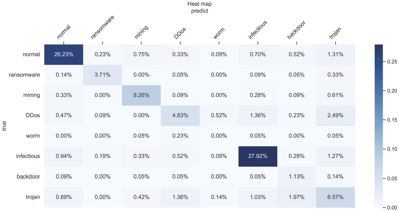
Table 5 presents a comparison of the classification results on dataset from catak’s work.
In our experiment, on the tianchi dataset, our method achieved a 6.94% improvement in accuracy, a 6.7% improvement in F1-score, a 6.94% improvement in recall and an 8.31% improvement in precision compared with catak’s method. On the dataset from catak’s work, our method achieved a 6.77% improvement in F1-score, a 7.38% improvement in recall, a 3.49% improvement in accuracy and a 3.88% improvement in precision compared with Catak’s method. Similarily, our method outperformed Ye’s methods in all metrics as well. We believe that our approach outperformed these models for two reasons. Firstly, our scenario is more suitable for few-shot learning as opposed to large models, which are prone to overfitting. Secondly, we utilized multi-task learning to further enhance the classification ability of our model.
4.Discussion
In this section, we have discussed the details of model construction and optimization, Including the selection of important substructures, optimization of related hyperparameters, and the utilization of multi-task strategies. The malware classification dataset was used as the benchmark for all the sub-sections. Except the final models, eight models were built for optimizing the structure of the model, and four comparisons were performed.
4.1.The distribution of the sample pairs
To represent API sequences as tensors, we used a one-hot representation, similar to natural language processing problems. Therefore, the rationality of data preprocessing is an important part of our malware detection work. To confirm that the one-hot feature is different from random generation, we made a comparison between one-hot representation and randomly generated samples using the mutual information [3] of the sample pairs. Similar to the dataset, a total of 10,654 random samples were generated to compute the mutual information, and
Fig. 9.
Distribution of mutual information between all preprocessed samples.

4.2.Length of feature sequence
Currently, methods used to process sequential data, such as graph convolutional neural networks, LSTM, and even random forests, require a fixed length for further computation. The length of the fixed sequence is a crucial characteristic of the model. If the length of the API call sequence is too short, it may lead to insufficient feature information, which can impact the detection accuracy. On the other hand, If the duration of the API call sequence is too long, the model easily falls into a tracking loop [21]. As shown in Fig. 10, the majority of samples have an API call sequence length of less than 300 in the histogram. Therefore, we compared our method, SGENext, SGEPre, LSTM network, and random forest detection methods for different sequence lengths ranging from 50 to 300 (as shown in Fig. 11, Fig. 12 and Fig. 13).
Fig. 10.
API call sequence length distribution of samples in tianchi dataset.
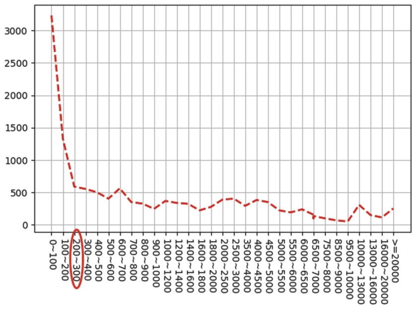
Fig. 11.
SGENext selects the performance with different sequence lengths in (a), SGEPre selects the performance with different sequence lengths in (b), our method selects the performance with different sequence lengths in (C).
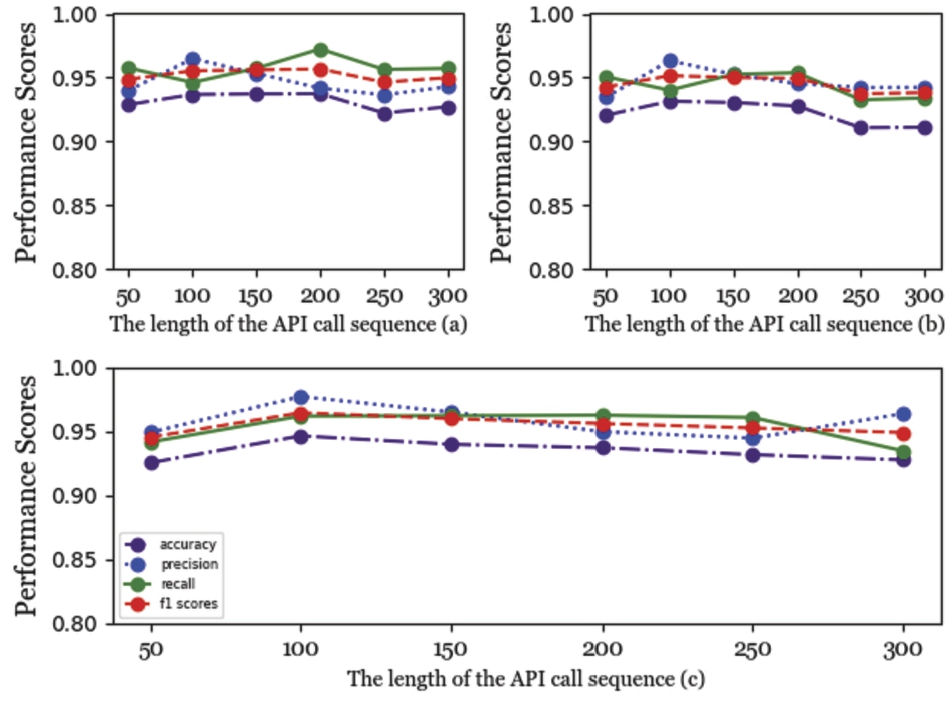
Fig. 12.
LSTM-based method selects the performance with different sequence lengths.
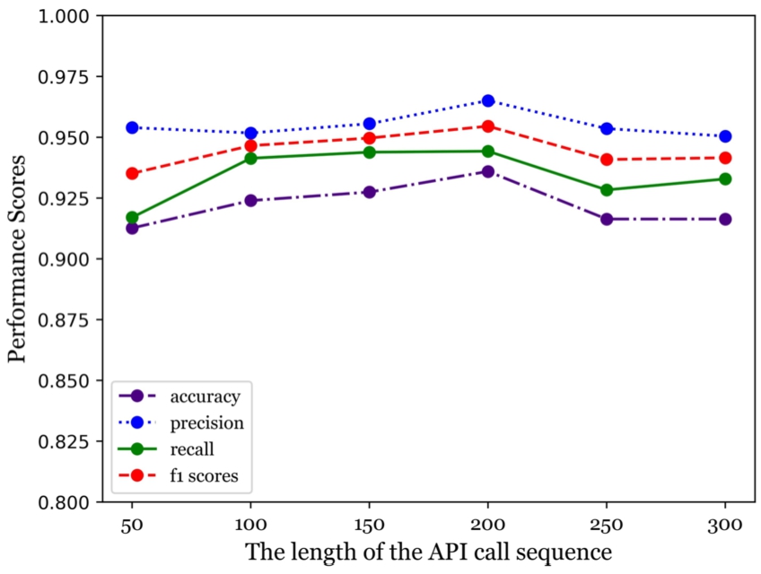
Fig. 13.
RF-based method selects the performance with different sequence lengths.
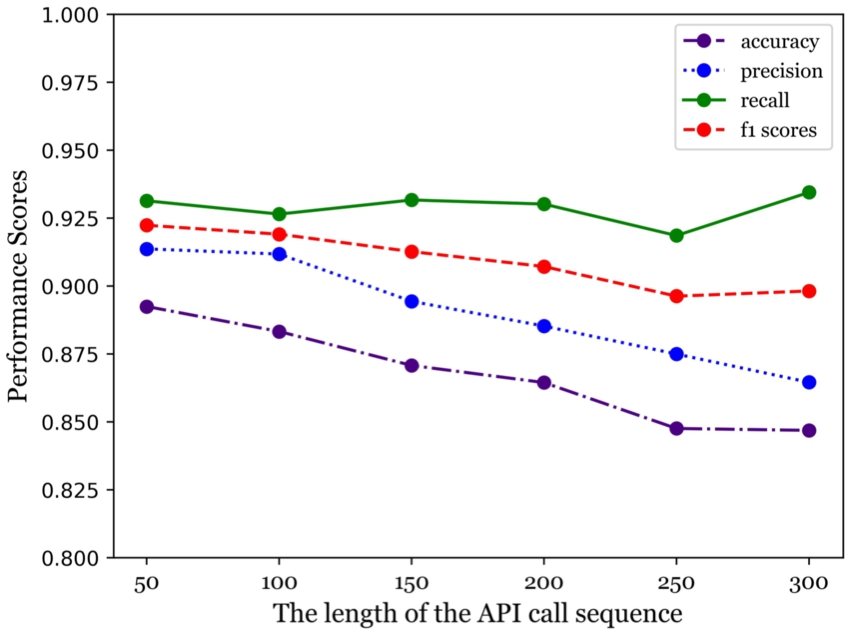
As seen from Fig. 11, Fig. 12 and Fig. 13, when the length of the feature sequence of the three machine learning methods involved changes, the range can be observed according to the plots. Figures 11, 12, and 13 show the performance trend of five different machine learning methods for different sequence lengths. Based on the plots, we can observe the range of performance for each method as the length of the feature sequence changes. After analyzing the performance trends of the five methods for different sequence lengths, we selected the optimal sequence length for each method. Our method was found to perform best at a sequence length of 100, while SGENext and SGEPre performed best at a sequence length of 200. The LSTM method also performed best at a sequence length of 200. However, the RF method performed best at the shortest sequence length of 50.
4.3.The direction of graph embedding
As mentioned in section ‘Directional Graph Embedding Module’, we use two directional graph embeddings, and the direction is a hyperparameter when using graph embedding. To investigate the effect of direction, we compared the performance of our method with SGENext and SGEPre (as shown in Table 6). In our experiment, our method achieved an accuracy rate that is 1.95% higher, an F1-score that is 2.04% higher, a recall that is 1.95% higher and a precision rate that is 3.98% higher than SGENext. Furthermore, the four evaluation metrics of our method are slightly better than SGEPre. Comparing the performance of SGENext and SGEPre reveals a certain difference between their performance. Therefore, it is meaningful and necessary to fully consider the direction of graph embedding when building the model.
Table 6
Classification results in different embedding directions
| Metric/model | Our method | SGENext | SGEPre |
| Precision | 0.8021 | 0.7623 | 0.7837 |
| Recall | 0.7957 | 0.7762 | 0.7874 |
| Accuracy | 0.7957 | 0.7762 | 0.7874 |
| F1-Score | 0.7896 | 0.7692 | 0.7855 |
4.4.The number of LSTM layers
A Bi-LSTM was used as the layer for feature learning and information processing. However, the outputs from a Bi-LSTM layer can be used as input to another Bi-LSTM layer, which means that using multiple Bi-LSTM layers is possible for modeling sequential data. According to Wang’s research, using multiple Bi-LSTM layers enhances the learning ability, especially for high-level sequence representation [21]. However, too many layers can result in a large number of parameters, leading to high computing cost and memory occupation. To determine the relation between the layer number and prediction performance, we compared the different models with only one, two, three and four Bi-LSTM layers. The hidden sizes of the LSTM layers were calculated as
Table 7
Classification results of used number of LSTM layers
| Metric/model | Single layer | Two layers | Three layers | Four layers |
| Precision | 0.7722 | 0.7740 | 0.8021 | 0.6271 |
| Recall | 0.7818 | 0.7813 | 0.7957 | 0.590 |
| Accuracy | 0.7818 | 0.7813 | 0.7957 | 0.7616 |
| F1-Score | 0.7769 | 0.7776 | 0.7896 | 0.6079 |
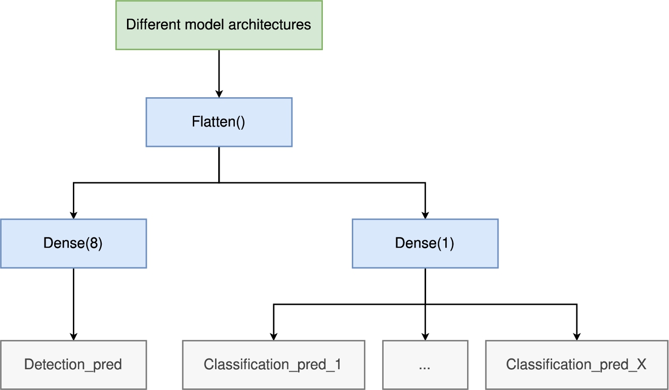
4.5.The architecture of multi-task learning
Using Multi-task Learning strategy is flexible since all the related attributes can be used for generating auxiliary loss. However, too many attributes will create unnecessary gradient due to the relation of the major targets. After few attempts, we constructed two models according to different strategies introduced in Section 2.4. The two models were named ‘multi-one-many model (MMany model)’ and ‘multi-paired model (MPaired model)’. As shown in Fig. 14, MMany model used a categorical cross entropy loss for identifying all eight classes and eight binary cross entropy losses for identifying a certain class of malware. MPaired model used a categorical cross entropy loss for all eight classes as well, but the aux-losses become 28 binary cross entropy losses for all malware class pairs (i.e.,
4.6.The difference between a CNN-LSTM-CNN architecture and CNN-LSTM architecture
Technically, the order of using LSTM and CNN layers is not limited since these layers do not reduce the dimension of the data. However, LSTM layers are designed to capture the global information from a sequence (i.e., the cell state) and process the data using the updated hidden information, while CNN layers capture local information surrounding a certain point every time. Therefore, it is necessary to compare the order of using the two types of neural network structures.
In our method, we first used a CNN layer as an information fusion encoder for initial data procession, followed by an RNN block containing three Bi-LSTM layers with a SeqSelfAttention layer after each was implemented. After the RNN block, we compared the performance of using an additional CNN layer or not (as shown in Fig. 15 and Fig. 16).
Fig. 15.
CNN-LSTM architecture.
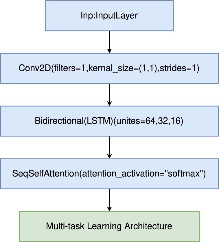
Fig. 16.
CNN-LSTM-CNN architecture.
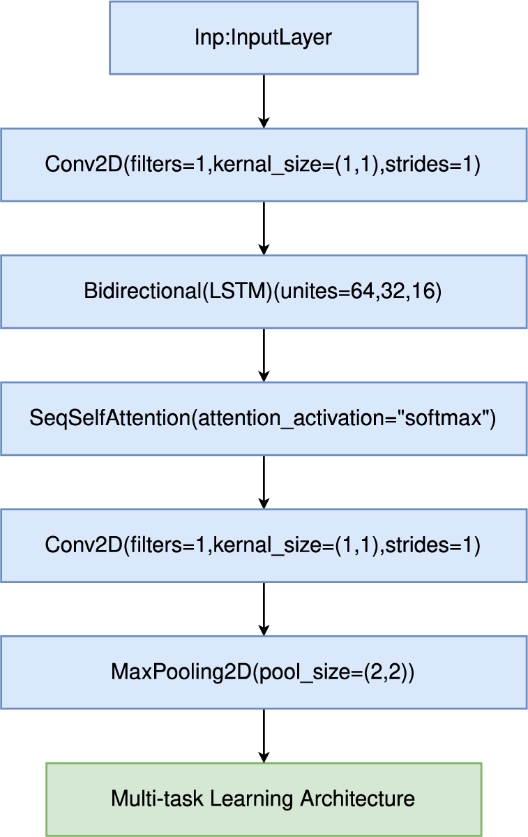
The result is depicted in Table 8. For our detection model, the architecture without a CNN layer after the Bi-LSTM layer performed the best. The comparison indicated that the LSTM layers have made the information separately of the sequences, but the additional CNN layer makes the information fuzzy again. Thus, we used the structure without the extra CNN layer as the final architecture.
Table 8
Result of using additional CNN layer
| Metric/model | CNN-LSTM | CNN-LSTM-CNN |
| Precision | 0.8021 | 0.7723 |
| Recall | 0.7957 | 0.7813 |
| Accuracy | 0.7957 | 0.7813 |
| F1-Score | 0.7896 | 0.7768 |
4.7.Different multi-task learning strategies
To compare various multi-task learning strategies, we included a model that performs a single task in Table 9 as a point of comparison. In our classification task, we compared two multi-task learning strategies: the MMany model and the MPaired model, as shown in Table 9. The MMany model provided eight extra binary classification sub-tasks by regarding the eight kinds of malware as positive labels, while the MPaired model used 28 binary classification sub-tasks to make the classification more detailed. We found that the first multi-task learning strategy (MMany model) performed better than the second multi-task learning strategy (MPaired model). The comparison indicates that too detailed sub-task division will not always make a positive contribution to the model. We speculate that the reason might be the unbalanced dataset and similarity between the classes. However, it is clear that using multi-task learning significantly improves the performance compared to the single-task situation. The evaluation metrics of the two multi-task models are globally better than the single-task model.
Table 9
Comparison of different multi-task models
| Metric/model | MMany model | MPaired model | Single task |
| Precision | 0.8021 | 0.7688 | 0.7338 |
| Recall | 0.7957 | 0.773 | 0.7457 |
| Accuracy | 0.7957 | 0.773 | 0.7459 |
| F1-Score | 0.7896 | 0.7709 | 0.7397 |
5.Future works
We analyzed the confusion matrix shown in Fig. 8 and found that the most recognized malware category is Ransomware, while the least recognized category is the Worm and Backdoor program. Despite the small number of Worm samples, the model’s prediction results showed that the classification results of backdoor programs and Trojan horse programs are not ideal, possibly due to the small number of samples. Moreover, the classification performance of Trojan horse programs and DDoS Trojan horse programs is poor. Therefore, in future work, we plan to carry out further research on the above three types of malware: backdoor programs, Trojan horse programs, and DDoS Trojan horse programs.
6.Related works
The field of malware classification and detection is typically divided into two main categories: static detection and dynamic detection. Static analysis involves extracting information from the file’s PE headers, such as dynamic link libraries, import tables, and export tables, and then using rules or blacklists to match these features and determine if the file is malicious. Dynamic analysis focuses on analyzing the behavior of malware by executing it in a controlled environment, such as a sandbox, and monitoring its actions to record execution information [39].
6.1.Dynamic analysis methods
During the last several years, several researchers have proposed various methods for detecting malware. Ye et al. [41] proposed a malware detection method based on malicious API sequence mining. This method extracted the dynamic API call sequences by simulating a real runtime environment for the malware and then mined out the pattern of the API sequence as features to classify the malware variants. Gupta and Rani [12] designed two methods based on ensemble learning and big data for malware detection, and they determined a set of integrated static and dynamic features based on malware classification and the software dataset. Tobiyama et al. [35] proposed a malware detection method based on process behavior logs, converting process behavior logs into vectors, using an RNN to convert them into feature images, and using a CNN to classify these feature images. Baek et al. [2] proposed a two-stage hybrid malware detection (2-MaD) scheme, which uses Opcode, API calls, and process memory as features to detect malware. Jiang et al. [17] proposed a new method that employs two stacked denoising autoencoders (SDAs) for representation learning, taking into consideration computer programs’ function-call graphs and Windows application programming interface (API) calls.
6.2.Malware detection with graph neural networks
Graph neural networks have gained popularity in recent years as a method for constructing deep learning models for malware classification. Xiao et al. [40] visualize malware binaries as entropy graphs based on structural entropy and present a feature extractor based on deep convolutional neural networks to extract patterns shared by a family from entropy graphs automatically. They propose an SVM classifier to classify malware based on the extracted features. Busch et al [5] propose an approach that first extracts flow graphs and subsequently classifies them using a novel edge feature-based graph neural network model. In this work, they propose the first graph-based approach to network traffic-based malware detection and classification, and propose a novel method for extracting directed edge attributed flow graphs from sets of network flows recorded in a monitored network. Some articles [42] propose using Generative Adversarial Network (GAN) combined with graph neural network to combat adversarial attacks. They retrain the model with generated adversarial samples. This work uses Graph Neural Networks (GNN)-based classifiers to generate API graph embedding and demonstrate the effectiveness of GNN in generating graph embedding. Zheng et al. [44] constructs a malware classifier by constructing different graph isomorphic networks and uses a simulated in-the-wild dataset as the test environment.
6.3.Methods available for comparison
The mentioned methods above have various characteristics in malware detection. However, in the method proposed in this work, only API call sequences were used for modeling, which limits comparability of our results to models that use the same dataset. Therefore, we compared our model with the models from Catak et al. [7], Oliveira et al. [30] and Ye et al. [41], the results are shown in Table 2, Table 3, Table 4 and Table 5 for both malware detection and classification.
7.Conclusion
In this work, we proposed a graph embedding method that uses API sequences to construct directed graphs. We applied multitasking learning to the complex problem of malware detection and classification, and the results showed that our proposed method outperforms other methods. We believe that using multitasking can improve the performance of multi-label classification with proper optimization and can be applied to related work in the field of malware detection and classification.
Notes
Acknowledgments
The authors would like to thank the journal reviewers for their valuable suggestions.
References
[1] | Y.A. Ahmed, B. Koçer, S. Huda, B.A.S. Al-rimy and M.M. Hassan, A system call refinement-based enhanced minimum redundancy maximum relevance method for ransomware early detection, Journal of Network and Computer Applications 167: ((2020) ), 102753. doi:10.1016/j.jnca.2020.102753. |
[2] | S. Baek, J. Jeon, B. Jeong and Y.-S. Jeong, Two-stage hybrid malware detection using deep learning, Human-centric Computing and Information Sciences 11: (27) ((2021) ), 10–22967. |
[3] | M.I. Belghazi, A. Baratin, S. Rajeshwar, S. Ozair, Y. Bengio, A. Courville and D. Hjelm, Mutual information neural estimation, in: International Conference on Machine Learning, PMLR, (2018) , pp. 531–540. |
[4] | L. Breiman, Random forests, Machine learning 45: ((2001) ), 5–32. doi:10.1023/A:1010933404324. |
[5] | J. Busch, A. Kocheturov, V. Tresp and T. Seidl, Nf-gnn: Network flow graph neural networks for malware detection and classification, in: 33rd International Conference on Scientific and Statistical Database Management, (2021) , pp. 121–132. doi:10.1145/3468791.3468814. |
[6] | R. Caruana, Multitask Learning, (1998) . |
[7] | F.O. Catak, A.F. Yazı, O. Elezaj and J. Ahmed, Deep learning based sequential model for malware analysis using windows exe API calls, PeerJ Computer Science 6: ((2020) ), e285. doi:10.7717/peerj-cs.285. |
[8] | Y. Ding, X. Xia, S. Chen and Y. Li, A malware detection method based on family behavior graph, Computers & Security 73: ((2018) ), 73–86. doi:10.1016/j.cose.2017.10.007. |
[9] | F. Fasano, F. Martinelli, F. Mercaldo and A. Santone, Energy consumption metrics for mobile device dynamic malware detection, Procedia Computer Science 159: ((2019) ), 1045–1052. doi:10.1016/j.procs.2019.09.273. |
[10] | A. Graves, N. Jaitly and A-R. Mohamed, Hybrid speech recognition with deep bidirectional LSTM, in: 2013 IEEE Workshop on Automatic Speech Recognition and Understanding, IEEE, (2013) , pp. 273–278. doi:10.1109/ASRU.2013.6707742. |
[11] | K. Griffin, S. Schneider, X. Hu and T.-C. Chiueh, Automatic generation of string signatures for malware detection, in: RAID, Vol. 5758: , Springer, (2009) , pp. 101–120. |
[12] | D. Gupta and R. Rani, Improving malware detection using big data and ensemble learning, Computers & Electrical Engineering 86: ((2020) ), 106729. doi:10.1016/j.compeleceng.2020.106729. |
[13] | W. Han, J. Xue and K. Qian, A novel malware detection approach based on behavioral semantic analysis and LSTM model, in: 2021 IEEE 21st International Conference on Communication Technology (ICCT), IEEE, (2021) , pp. 339–343. doi:10.1109/ICCT52962.2021.9658113. |
[14] | S.S. Hansen, T.M.T. Larsen, M. Stevanovic and J.M. Pedersen, An approach for detection and family classification of malware based on behavioral analysis, in: 2016 International Conference on Computing, Networking and Communications (ICNC), IEEE, (2016) , pp. 1–5. |
[15] | X. Huang, L. Ma, W. Yang and Y. Zhong, A method for windows malware detection based on deep learning, Journal of Signal Processing Systems 93: ((2021) ), 265–273. doi:10.1007/s11265-020-01588-1. |
[16] | J. Hwang, J. Kim, S. Lee and K. Kim, Two-stage ransomware detection using dynamic analysis and machine learning techniques, Wireless Personal Communications 112: ((2020) ), 2597–2609. doi:10.1007/s11277-020-07166-9. |
[17] | H. Jiang, T. Turki and J.T. Wang, DLGraph: Malware detection using deep learning and graph embedding, in: 2018 17th IEEE International Conference on Machine Learning and Applications (ICMLA), IEEE, (2018) , pp. 1029–1033. doi:10.1109/ICMLA.2018.00168. |
[18] | A. Kendall, Y. Gal and R. Cipolla, Multi-task learning using uncertainty to weigh losses for scene geometry and semantics, in: Proceedings of the IEEE Conference on Computer Vision and Pattern Recognition, (2018) , pp. 7482–7491. |
[19] | H. Kim, J. Kim, Y. Kim, I. Kim, K.J. Kim and H. Kim, Improvement of malware detection and classification using API call sequence alignment and visualization, Cluster Computing 22: ((2019) ), 921–929. doi:10.1007/s10586-017-1110-2. |
[20] | T.N. Kipf and M. Welling, Semi-supervised classification with graph convolutional networks, (2016) , arXiv preprint arXiv:1609.02907. |
[21] | B. Kolosnjaji, A. Zarras, G. Webster and C. Eckert, Deep learning for classification of malware system call sequences, in: AI 2016: Advances in Artificial Intelligence: 29th Australasian Joint Conference, Proceedings 29, Hobart, TAS, Australia, December 5–8, 2016, Springer, (2016) , pp. 137–149. doi:10.1007/978-3-319-50127-7_11. |
[22] | A. Kumar, K. Kuppusamy and G. Aghila, A learning model to detect maliciousness of portable executable using integrated feature set, Journal of King Saud University-Computer and Information Sciences 31: (2) ((2019) ), 252–265. doi:10.1016/j.jksuci.2017.01.003. |
[23] | Y. LeCun, Y. Bengio and G. Hinton, Deep learning, nature 521: (7553) ((2015) ), 436–444. doi:10.1038/nature14539. |
[24] | B. Li, K. Roundy, C. Gates and Y. Vorobeychik, Large-scale identification of malicious singleton files, in: Proceedings of the Seventh ACM on Conference on Data and Application Security and Privacy, (2017) , pp. 227–238. doi:10.1145/3029806.3029815. |
[25] | Y.T. Ling, N.F.M. Sani, M.T. Abdullah and N.A.W.A. Hamid, Nonnegative matrix factorization and metamorphic malware detection, Journal of Computer Virology and Hacking Techniques 15: ((2019) ), 195–208. doi:10.1007/s11416-019-00331-0. |
[26] | L. Liu, B.-S. Wang, B. Yu and Q.-X. Zhong, Automatic malware classification and new malware detection using machine learning, Frontiers of Information Technology & Electronic Engineering 18: (9) ((2017) ), 1336–1347. doi:10.1631/FITEE.1601325. |
[27] | E. Menahem, A. Shabtai, L. Rokach and Y. Elovici, Improving malware detection by applying multi-inducer ensemble, Computational Statistics & Data Analysis 53: (4) ((2009) ), 1483–1494. doi:10.1016/j.csda.2008.10.015. |
[28] | Q.K.A. Mirza, I. Awan and M. Younas, CloudIntell: An intelligent malware detection system, Future Generation Computer Systems 86: ((2018) ), 1042–1053. doi:10.1016/j.future.2017.07.016. |
[29] | B. Ndibanje, K.H. Kim, Y.J. Kang, H.H. Kim, T.Y. Kim and H.J. Lee, Cross-method-based analysis and classification of malicious behavior by api calls extraction, Applied Sciences 9: (2) ((2019) ), 239. doi:10.3390/app9020239. |
[30] | A. Oliveira and R. Sassi, Behavioral malware detection using deep graph convolutional neural networks, TechRxiv ((2019) ), preprint. |
[31] | R. Pascanu, J.W. Stokes, H. Sanossian, M. Marinescu and A. Thomas, Malware classification with recurrent networks, in: 2015 IEEE International Conference on Acoustics, Speech and Signal Processing (ICASSP), IEEE, (2015) , pp. 1916–1920. doi:10.1109/ICASSP.2015.7178304. |
[32] | J. Saxe and K. Berlin, Deep neural network based malware detection using two dimensional binary program features, in: 2015 10th International Conference on Malicious and Unwanted Software (MALWARE), IEEE, (2015) , pp. 11–20. doi:10.1109/MALWARE.2015.7413680. |
[33] | M. Schofield, G. Alicioglu, R. Binaco, P. Turner, C. Thatcher, A. Lam and B. Sun, Convolutional neural network for malware classification based on API call sequence, in: Proceedings of the 8th International Conference on Artificial Intelligence and Applications (AIAP 2021), (2021) . |
[34] | P. Shijo and A. Salim, Integrated static and dynamic analysis for malware detection, Procedia Computer Science 46: ((2015) ), 804–811. doi:10.1016/j.procs.2015.02.149. |
[35] | S. Tobiyama, Y. Yamaguchi, H. Shimada, T. Ikuse and T. Yagi, Malware detection with deep neural network using process behavior, in: 2016 IEEE 40th Annual Computer Software and Applications Conference (COMPSAC), Vol. 2: , IEEE, (2016) , pp. 577–582. doi:10.1109/COMPSAC.2016.151. |
[36] | S. Vandenhende, S. Georgoulis, M. Proesmans, D. Dai and L. Van Gool, Revisiting multi-task learning in the deep learning era, Vol. 2, (2020) , arXiv preprint arXiv:2004.13379. |
[37] | R. Vinayakumar, M. Alazab, K. Soman, P. Poornachandran and S. Venkatraman, Robust intelligent malware detection using deep learning, IEEE Access 7: ((2019) ), 46717–46738. doi:10.1109/ACCESS.2019.2906934. |
[38] | J. Wang, M. Xu, H. Wang and J. Zhang, Classification of imbalanced data by using the SMOTE algorithm and locally linear embedding, in: 2006 8th International Conference on Signal Processing, Vol. 3: , IEEE, (2006) . |
[39] | T. Wuechner, A. Cisłak, M. Ochoa and A. Pretschner, Leveraging compression-based graph mining for behavior-based malware detection, IEEE Transactions on Dependable and Secure Computing 16: (1) ((2017) ), 99–112. doi:10.1109/TDSC.2017.2675881. |
[40] | G. Xiao, J. Li, Y. Chen and K. Li, MalFCS: An effective malware classification framework with automated feature extraction based on deep convolutional neural networks, Journal of Parallel and Distributed Computing 141: ((2020) ), 49–58. doi:10.1016/j.jpdc.2020.03.012. |
[41] | Y. Ye, L. Chen, S. Hou, W. Hardy and X. Li, DeepAM: A heterogeneous deep learning framework for intelligent malware detection, Knowledge and Information Systems 54: ((2018) ), 265–285. doi:10.1007/s10115-017-1058-9. |
[42] | R. Yumlembam, B. Issac, S.M. Jacob and L. Yang, Iot-based android malware detection using graph neural network with adversarial defense, IEEE Internet of Things Journal ((2022) ). |
[43] | D. Yuxin and Z. Siyi, Malware detection based on deep learning algorithm, Neural Computing and Applications 31: ((2019) ), 461–472. doi:10.1007/s00521-017-3077-6. |
[44] | R. Zheng, Q. Wang, J. He, J. Fu, G. Suri and Z. Jiang, Cryptocurrency Mining Malware Detection Based on Behavior Pattern and Graph Neural Network, Security and Communication Networks 2022 ((2022) ). doi:10.1155/2022/8288855. |

