A Grey-box model approach using noon report data for trim optimization

Zwart, Robert H.; Bogaard, Jordi; Kana, Austin A.

doi:10.3233/ISP-220009

A Grey-box model approach using noon report data for trim optimization

Article type: Research Article

Authors: Zwart, Robert H.^{a; *} | Bogaard, Jordi^a | Kana, Austin A.^{b; **}

Affiliations: [a] Stolt Tankers, Rotterdam, the Netherlands | [b] Delft University of Technology, Department of Maritime and Transport Technology, Delft, the Netherlands

Correspondence: [**] Corresponding author. E-mail: a.a.kana@tudelft.nl.

Note: [*] Work performed at Delft University of Technology, Delft, the Netherlands.

Keywords: Trim optimization, grey-box modelling, sea-trial validation, noon reports, chemical tankers

DOI: 10.3233/ISP-220009

Journal: International Shipbuilding Progress, vol. 70, no. 1, pp. 41-63, 2023

Received 20 October 2022

Revision received 17 May 2023

Accepted 25 May 2023

Published: 22 June 2023

Get PDF

Abstract

Trim optimization improves the energy efficiency of ships, thus reducing operational costs and emissions; however, trim tables are only available for a limited number of ships. There is thus a desire to develop additional, more accurate trim tables without the need for expensive model testing. The objective of this research was to develop a method to decrease fuel consumption by trim optimization, by a dynamic shaft power estimation model based on available operational data. A method that uses noon report data and a grey-box modelling approach is proposed. The grey box model consists of a multi-layer feedforward neural network to estimate the required shaft power, using operational parameters and an initial estimate of the required shaft power. A case study is presented for a modern chemical tanker and sea trials have been conducted to validate the results. The method provides correct trim advice for full load conditions; however, the magnitude of the effect is smaller compared to sea trial results. The model is able to estimate the required power with an average accuracy of over 6% for a random subset of the noon report data. Due to challenges inherent to noon reports as a data source, the actual effect of trim and speed have a bigger magnitude than the extracted trend.

1.Introduction

The IMO [13] has set the goal that greenhouse gas (GHG) emissions from international shipping should peak as soon as possible and should be reduced by 50% by 2050 compared to 2008, consistent with the Paris Agreement of the United Nations [23]. GHG emissions from the combustion of oil-based fuels are directly proportional to fuel consumption, which makes improving the ship’s energy efficiency one of the possible solutions to reduce GHG emissions [4]. To reduce GHG emissions, the Marine Environment Protection Committee (MEPC) of IMO adopted a strategy, in which shipping companies are supported to improve the energy efficiency operational index (EEOI) of their ships in operation [12]. Trim optimization is one of the approaches considered by the industry to improve the energy efficiency of ships, thereby having the potential to both reduce operational costs and in reducing the emissions of the ship. Trim optimization is the selection of trim with the goal of fuel consumption reduction, by ballast water management and load distribution, which can be done without significant changes to the ship structure [4,9,14].

The MEPC [17] estimates that optimization of trim and draft can reduce the fuel consumption by 0.5% to 3% on main engine fuel consumption for most vessel types. For ships with partial loads, this can be as high as 5%. Coraddu et al. [4] conclude that improvements exceeding 2% in fuel consumption for a handymax chemical tanker can be achieved and DNV-GL [6] records savings between 2% and 14% for different draft and speed combinations of a handymax bulk carrier. Therefore, it can be stated that to achieve an effective and significant fuel consumption reduction by trim optimization a comprehensive study should be performed on several ship types, considering appropriate operative profiles.

Multiple approaches exist to determine the optimal trim for given load conditions. Approaches using model scale data, i.e. model scale towing tests or CFD simulations, inherently suffer from scaling effects and need to be performed for every ship hull shape again when trim optimization is to be used for other ships. Moreover, these approaches generally assume calm water conditions, while the influence of trim on fuel consumption in reality also depends on weather and sea conditions [1,4,7,14].

On the other hand, ship-scale data can be used. Ship-scale data can be divided into continuous measurements (CM) and noon report (NR) data. CM data are considered to provide accurate data, but typically require additional instruments and sensors not readily available on most ships. NR data, on the other hand, are considered to be a readily available data source. This research supports the idea that it would be of additional value for the industry to develop a method to perform trim optimization based on NR data. It should be noted, however, that the quality of NR data may be a concern [2]. Human error is a source of noise in observing and recording the required data fields and a mismatch exists between the snapshot of conditions on one hand, and the 24-hr averaged sailing speed and recorded shaft power or fuel consumption on the other hand. The goal of this research is to improve existing methods of using NR data for trim optimization.

2.Review of modelling strategies for fuel consumption estimation

Multiple approaches exist to develop models that could estimate either the fuel consumption for propulsion or required propulsion power in various conditions, referred to as fuel consumption modelling. The approaches can be divided into white-box model (WBM) approaches, black-box model (BBM) approaches and grey-box model (GBM) approaches.

2.1.White-box modelling (WBM)

Fuel consumption modelling can be done by applying physics-based relations and relations found by regression analysis from the model and full-scale experiments. This approach is known as white-box modelling (WBM). WBMs are generally rather tolerant to extrapolation, but the margin of error to estimate the fuel consumption for a specific ship in realistic sailing conditions, especially considering wind and waves, can be large [4,15]. While the field of WBMs for fuel consumption is vast, the most relevant models for this work regards those for calm water resistance and those for hull forms relevant to chemical tankers, such as the well-known low-fidelity Admiralty coefficient, the method of Holtrop and Mennen [11] or the method of Lützen and Kristensen [16].

2.2.Black-box modelling (BBM)

Alternatively, it is possible to observe data to predict the output of a system given some input data, without the requirement to understand the system behaviour. This approach is described as black-box modelling (BBM). A BBM gives a functional relationship between system input and output, which does not represent any physical significance, and can be more effective to model trends in process behaviour [28]. Moreover, a BBM can be more accurate than a WBM, but requires large amounts of data for training and often suffers from poor extrapolation qualities [15,18,24,26]. The performance of a BBM depends on the dataset and problem being studied [8,25].

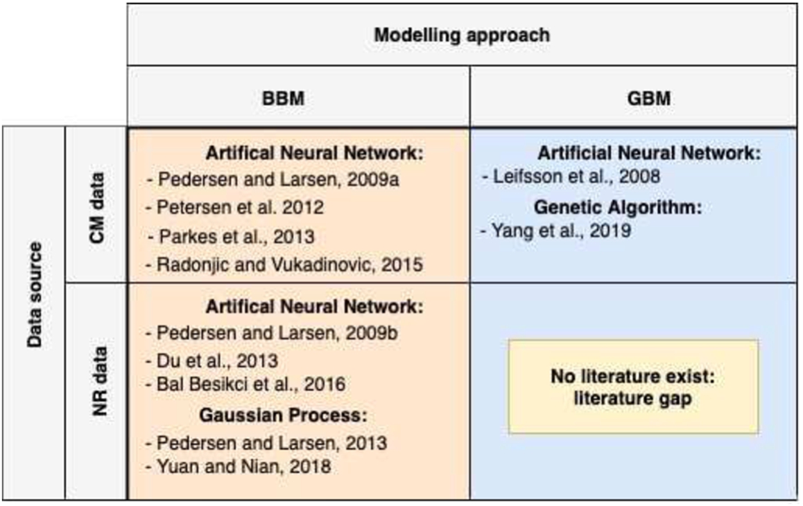
Applying a BBM approach to model propulsion power of fuel consumption based on NR data has been done by Du et al. [7], Bal Besikci et al. [3], and Pedersen and Larsen [19] using artificial neural networks (ANNs) and by Pedersen and Larsen [20] and Yuan and Nian [27] using Gaussian Process regression (GP). Petersen, et al. [21] investigated and compared the use of an ANN and GP, by using an operational high-frequency dataset of a ferry over a period of two months. In all tests performed in the paper, the performance of the ANN was a little better than the GP. Additionally, in the research of Pedersen and Larsen [20] and Yuan and Nian [27], it was found that similar accuracy can be obtained, although a GP is not appropriate for the analysis of large datasets because the complexity increases with the number of input parameters to the third power [20]. Moreover, in the case of an ANN, it is suggested that larger networks will improve the ability to extrapolate beyond the available input data [18]. This research has thus selected the use of an ANN over a GP for modelling fuel consumption based on noon report data.

Pedersen and Larsen [19] present an ANN to estimate the propulsion power of a 110,000 DWT tanker in various conditions. Different combinations of input variables are used, enabling the comparison of the effect of the selection of variables. Using NR data only resulted in an accuracy of about 7%. In the best case, combining NR data with hindcast weather data resulted in a model accuracy of about 2%. However, the available data set is split into four relatively small data sets with a limited range of conditions. Therefore, the accuracy is likely to decrease when new conditions are met.

The model of Du et al. [7] uses 10 input variables to model the daily fuel consumption for two 9000 TEU container ships based on NR data. The model accuracy has been expressed in terms of root mean square error (RMSE), which was 8.23 and 9.34 MT/day for both ships for the best performing developed ANN. As a reference, the average fuel consumption of one of the ships was approximately 74 MT/day, estimated based data description provided for one of the ships.

In addition, Bal Besikci et al. [3] present an ANN using 7 input variables to model the hourly fuel consumption of a 150,000 DWT oil tanker. The accuracy is expressed in an RMSE of 0.141 MT/h on a mean consumption of 1.89 MT/h. However, an alternative definition of RMSE is used.

The work of Parkes et al. [18] shows the potential of using CM data and ANNs in estimating the shaft power. Data of three sister vessels over a period of approximately two years are combined. The presented model was able to estimate the shaft power with a relative error of 7.8%. According to the authors, the accuracy will likely be better within the region of sufficient data points and less accurate in ‘extreme’ conditions. Other literature that use a BBM approach and CM data for fuel consumption modelling include Pedersen and Larsen [19], Petersen, et al. [21], and Radonjic and Vukadinovic [22].

2.3.Grey-box modelling (GBM)

Grey-box models (GBM) aim to combine the advantages of both a WBM and a BBM. The goal is to retain physics-based knowledge from the WBM according to its level of fidelity about the physical behaviour of the ship regarding the propulsion power and resistance, while the BBM integrates what is known from the specific operational data of the ship [15,26].

The advantages of GBMs over WBM and BBM as described by Yang et al. [26] are:

More accurate than a WBM by considering ship-specific, real operational conditions
Less historical data required than a BBM
A certain degree of extrapolation capacity
Can avoid unreasonable results because of over- or under fitting of available data.

The improved performance of a GBM over a WBM or a BBM in predicting fuel consumption of a ship, and the improved extrapolation capacity of a GBM over a BBM especially, is shown by the work of Leifsson et al. [15]. In [15], a GBM was constructed to model the fuel flow rate (samples every 15 s) of a cargo ship that operates between Iceland and Northern Europe. The ship typically operates with speeds between 18 and 20 knots. When the vessel operates at different sailing speeds than normal operations, the GBM predicts the fuel consumption closer to the actual data than the BBM, indicating better extrapolation results. It is described that the overall RMSE of the WBM is more than three times larger than the GBM.

A WBM and a BMM can be combined in two ways: in serial or in parallel [5]. In serial grey-box modelling, the BBM is provided with an initial estimation of the fuel consumption, which can be seen as an additional parameter for the BBM. In parallel grey-box modelling, the BBM models the residual of the measured and calculated fuel consumption. The authors evaluated both ways and found a marginal difference in outcome between the two.

2.4.Literature gap

Despite the potential to decrease fuel consumption by trim optimization based on NR data and the potential of improved capabilities of a GBM over a BBM, no research has been published, to the best of the authors’ knowledge, considering such an approach to extract knowledge from NR data for trim optimization purposes. The gap in the existing literature is illustrated in Fig. 1. This research focuses on a GBM approach using NR data.

Fig. 1.

Literature gap in fuel consumption modelling.

3.Method

3.1.Model variants

Two WBMs have been used and compared to make an initial estimate of the required shaft power. The first WBM uses the method of Lützen and Kristensen [16] for both the resistance estimation and the propulsive characteristics, which is described as PLK. The other WBM uses the method of Holtrop and Mennen [11] for resistance estimation and the method of Lützen and Kristensen [16] for propulsion characteristics. This WBM is described as PHM. The technical details of PLK and PHM can be found in their respective original sources [11,16]. It was found that the proposed method of Holtrop and Mennen [11] is hard to implement for a ship with a controllable pitch propeller (CPP), while the P/D-ratio is not recorded in the NR data. A third model variant consists of a pure BBM, to compare the results of GBM-PLK and GBM-PHM.

3.2.Data pre-processing

Data pre-processing is required to process the abundance of available data into usable input for the ANN. Garcia et al [10] distinguish six steps in data pre-processing for big-data analysis, which are data cleaning, transformation, integration, normalization, missing values imputation, and noise identification. Parkes et al [18] show the added value of a Spearman Rank correlation analysis for feature selection, which is adopted in the framework as well. Also, data selection is added as a step, as it has been found during the analysis that some additional data might be filtered out for specific reasons and the use of different datasets enables to perform additional comparisons. Finally, a sequential order is introduced. The final data pre-processing framework is shown in Fig. 2.

Fig. 2.

Data pre-processing framework (based on [5]).

The data pre-processing steps in group A start with the integration of the available data. Steps in group B consist of increasing the quality of the data. The steps of data selection in group C make it possible to filter for additional requirements. Feature selection has been done by the Spearman Rank analysis. The goal of this analysis is to prevent selecting redundant variables and to select the most strongly correlated variable between similar ones. Using input variables which are strongly correlated to each other, may result in the overfitting of these variables [18]. Finally, Da Silva et al. [5] recommend scaling the in- and output variables, to avoid saturation of the neurons. This is done according to the proportional segment principle, shown by Equation (1). Here z is the scaled value and x is the value from the NR.

(1)z=2∗(x−xminxmax−xmin)−1

3.3.Network training

The neural network toolbox of Matlab2017b has been used to train the neural network.

3.3.1.Network initialization

Three sets of data are composed from the available data points. A training set (70%) is used to train the network, a validation set (15%) is used to validate if the performance of the trained network has reached a stopping criterion and a test set (15%) is used to evaluate the performance with new data. Additionally, it is ensured that the extreme values of the input variables are within the training subset. Otherwise, if these extreme values are allocated to the test subset, the network tries to generalize values that are outside the domain of the input variables, causing significant errors [5].

3.3.2.Network settings

Different learning algorithms, all following a supervised learning strategy, have been used. The Bayesian Regularization training algorithm has shown to provide the most accurate and consistent results and was relatively fast. The hyperbolic sigmoid function has been used as the activation function. Network training was stopped when the network accuracy of the validation test set decreased for six consecutive epochs. Then the model accuracy was determined using the test subset. The accuracy of the model has been evaluated by calculating the mean relative error (REK‾) of all K relative errors of each Kth training subset, with all N noon reports in the test subset (see Equation (2)). Here, Yˆ is the estimated output value and Y is the actual output value known from the nth noon report.

(2)RE‾=1K1N∑k=1K∑n=1NYˆn−YnYn

3.3.3.Network topology

The final network topology has been determined empirically by a topology analysis, varying from one to four hidden layers with a range of several nodes in each layer. The Fletcher–Gloss method (Equation (3)) was used as a guideline for the number of neurons in the hidden layer(s) (n1), where n is the number of input variables and n2 the number of output variables.

(3)2∗n+n2⩽n1⩽2∗n+1

Performance has been measured in terms of relative accuracy and stability, in terms of the standard deviation between all k results. Because the performance depends on the data subset division, cross-validation is done by repeating the training algorithm k=100 times for new randomly sub-sampled data sets. The final network settings used in the model are summarized in Table 1.

Table 1

Neural network settings

Train function	Bayesian Regularization (‘trainbr’)
Hidden layer size	18 (GBM-PHM)
	15 (GBM-PLK)
	27 (BBM) as this was found optimal after network topology analysis for each model
Activation function	Hyperbolic sigmoid function
Max epochs	200
MSE goal	0.01/100
Max time	1200
Max consecutive validation failures (increase in mse)	6
Train ratio	0.7
Validation ratio	0.15
Test ratio	0.15

4.Case study model description

4.1.Case study data pre-processing

For this work, NR data of six sister vessels of a modern large chemical tanker have been collected over their lifetime, which is a period of 2 to 3.5 years, resulting in 2923 noon reports. Next to this, the days since the last hull cleaning and propeller polishing were collected, as well as ship-related information required for the WBMs. Wind, sea, and swell directions were recorded in points of the compass (N-NNE-NE-…) which had to be transformed into directions relative to the ship’s heading. Average ship speed is defined as the log distance through water per hour of the reporting period.

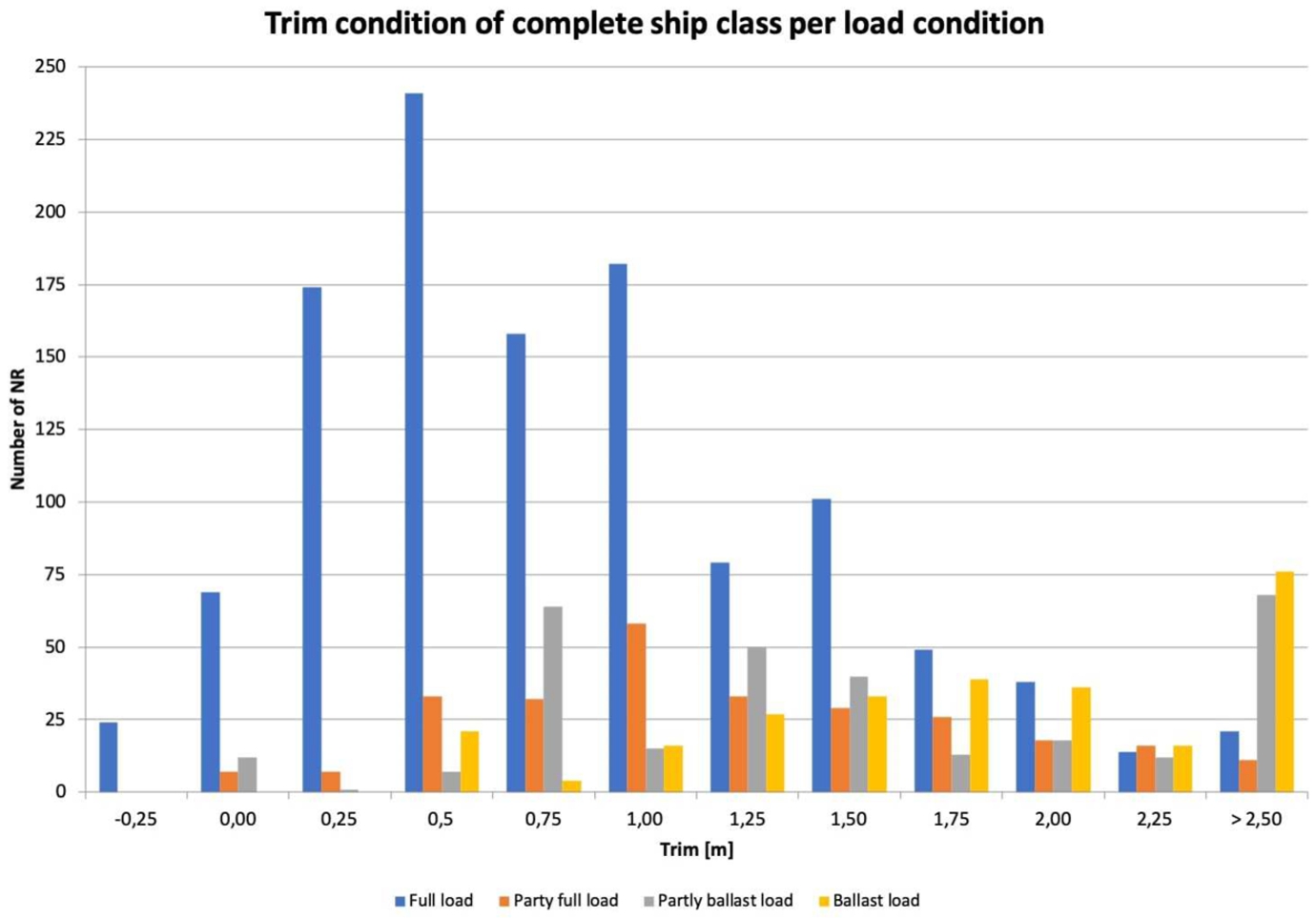
Logical rules have been applied to search for missing or deviating data entries. The recorded power is compared with the estimated power using the Admiralty coefficient, to find outliers in shaft power recordings. In this study, 935 NRs were deleted in these steps. The result of these steps is a cleaned data set, which is used to identify the boundaries of the model. A description of the draft and trim recordings is given in Fig. 3, which shows that in most cases (58%) the ship sails at a (near) full loaded condition, while other load conditions are sailed less frequently. At this condition, most trim conditions have been sailed, but noon reports with trim by bow are scarce. At other draft conditions, the ship is trimmed to the stern more often, which can be explained by the weight distribution of the ship.

Fig. 3.

Frequency histogram of load and trim conditions.

The step of data selection in group C makes it possible to filter for additional requirements. This has been done by composing two data sets, which enable to compare the results and understand the effect of the rough weather conditions on the model performance. The main data set represents all encountered weather conditions. The other data set represents calm water conditions, that fulfill the following two conditions:

A sea state of 3 on the scale of Douglas is taken as the upper bound, which relates to slight waves, with a wave height up to 1.25 m.
A swell state of 2 on the scale of Douglas is taken as the upper bound, which relates to low waves, defined as a swell height up to 2 m (lowest swell height on the scale of Douglas).

The result of the Spearman Rank analysis is shown in Fig. 4.

Fig. 4.

Spearman rank correlation for all weather conditions.

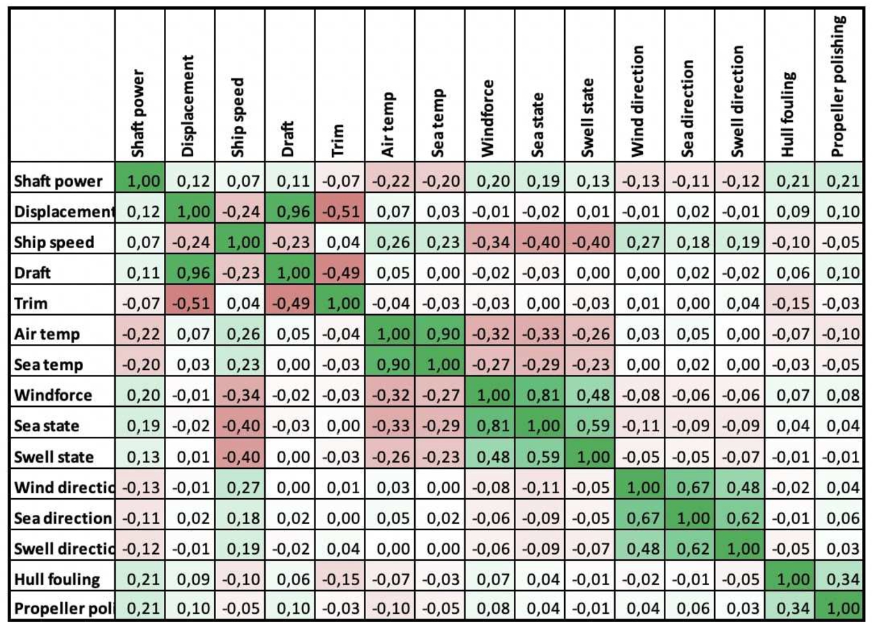
A third-order relation between ship speed and required power may be expected, therefore also a correlation between these factors may be expected. However, this relation is not found in the correlation analysis. Due to the nature of ship operation during voyages, the speed is more a result of engine settings and weather conditions. In rough conditions, the speed will vary more than in calm water conditions. The correlation was significantly stronger (+0.35) for the calm water dataset.

Sea water temperature is preferred over air temperature since the seawater temperature is less correlated with wind, sea and swell factors. Moreover, sea water temperature is required for the WBMs. Still, sea water temperature is correlated with wind, sea and swell factors. The result of taking such a variable into account has been observed with a trained network. The effect of seawater temperature was much bigger than can be explained by maritime physics only. Likely, low sea water temperature comes together with, in general, worse wind, sea and swell conditions. However, excluding this variable resulted in a drop in accuracy of about 0.2% of the model performance. Therefore, this variable is selected as well in the final feature selection. This small experiment has shown that variables that are correlated to each other do contribute to model performance, but the extracted effects are affected by the correlated variables. These lessons are useful for further model evaluation.

The selected variables are:

Speed through water (knots)
Mean draft (m)
Trim (m)
Sea water temperature (°C)
Wind force (Bf)
Relative wind direction (°)
Sea state (Douglas)
Relative sea direction (°)
Swell states (Douglas)
Relative swell direction (°)
Days since last hull cleaning
Days since last propeller polishing

Fig. 5.

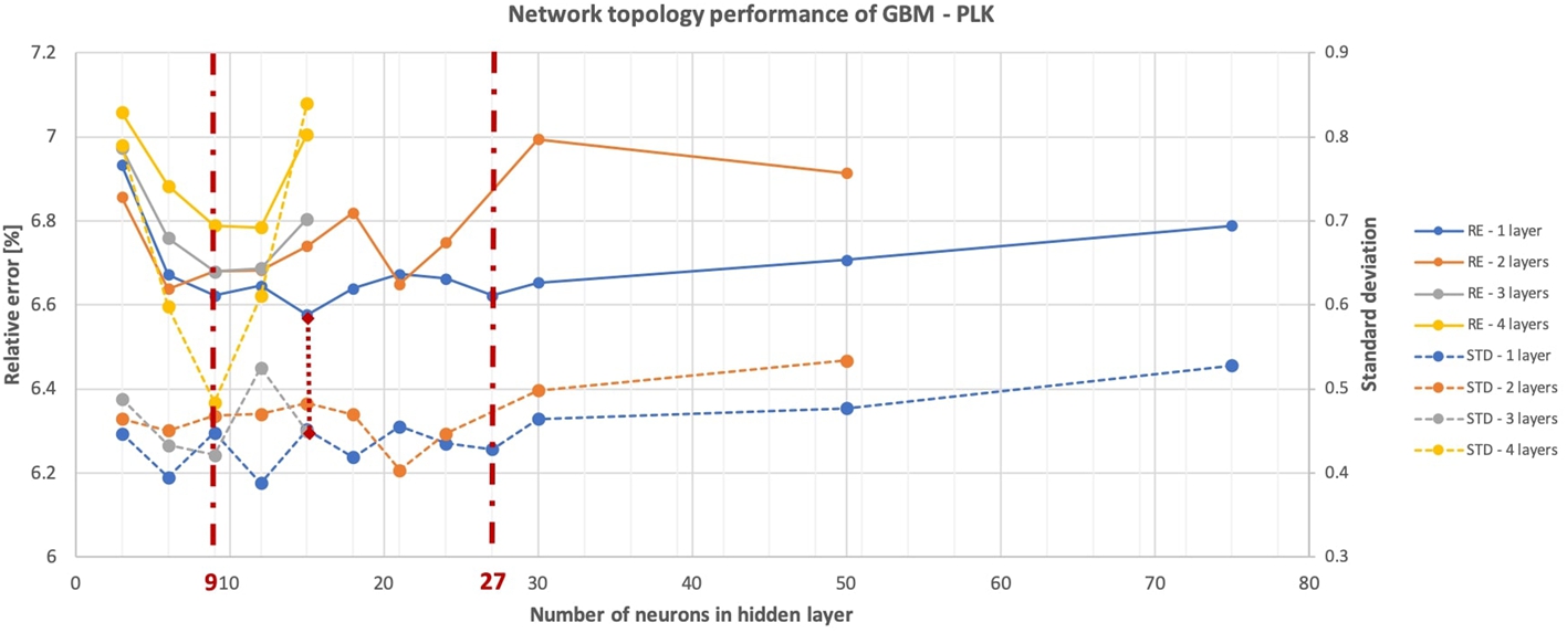
Topology analysis for the GBM – PLK model variant. The number of neurons in each hidden layer is represented by the x-axis. The relative error (RE) is represented by the left y-axis, the standard deviation between k results of the RE is represented on the right y-axis.

Table 2

Results of network topology analysis

	Optimality topology	RE	STD
GBM – PHM	1×18	6.62	0.431
GBM – PLK	1×15	6.58	0.452
BBM	1×27	6.63	0.417

4.2.Network topology (case study)

The results of the network topology analysis of one of the model variants are shown in Fig. 5. The topology analysis for the other two model variants showed very similar behaviour. Network topology and corresponding results are shown in Table 2. Generally, it is observed that the differences in performance between the three models are very small. In most cases, the use of one hidden layer provides a more accurate and stable network than a network with two hidden layers. Both the average relative error and the standard deviation of the relative errors of each training iteration is generally smaller. Relative error of the test set has been used as metric to evaluate the network topology performance. During the network topology analysis it was found that multiple layer network topologies tend to cluster estimations to a small range of mean values, indicating overfitting on the training data. Considering multiple hidden layers, the variability in estimated shaft power tends to be limited. Network topologies with three of four hidden layers tend to cluster estimations to a small bound of mean values and sometimes even provide one single shaft power for all speeds.

5.Model results

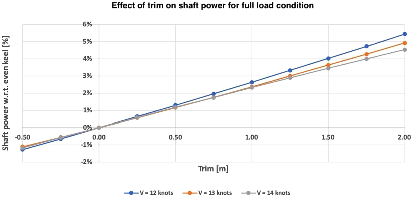
The model is able to estimate the required shaft power given a specified set of input variables. In that way, trim tables can be generated dynamically. For each combination of draft and trim, shaft power is estimated for one speed at a time, while taking into account the weather and fouling effects. For a full load condition and calm water conditions, the model results of the effect of trim on power are shown in Fig. 6. These results show that a linear effect between trim and shaft power is extracted from the noon report, showing that a bow trim of 0.5 m is optimal and can save approximately 1% (full load) to 2% (ballast load) of the required shaft power compared to even keel.

Fig. 6.

Model results regarding the effect of trim on shaft power for full load condition.

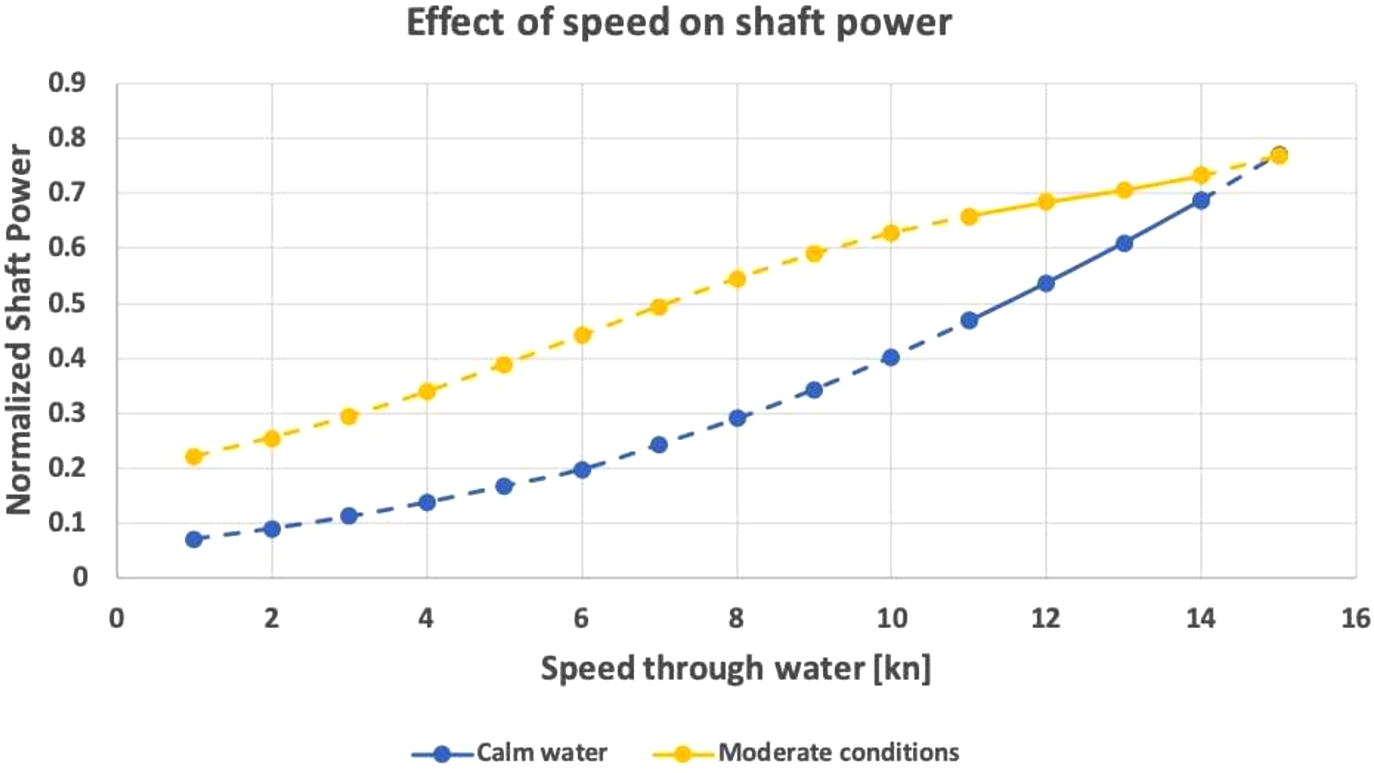
By varying one variable at a time, while keeping the other parameters constant, the effect of all variables on shaft power can be extracted. This approach has been used to understand the model behaviour. For example, in further simulations, it has been found that the effect of speed on shaft power was unrealistically small. The effect of speed on power is shown in Fig. 7, for calm water and moderate conditions. In the case of moderate conditions, the model attributes a significant effect of the weather and sea conditions on shaft power, causing an unrealistic relationship between ship speed and shaft power for speeds of 8 knots and more. This problem has not been solved yet within this research.

Fig. 7.

Model results regarding the effect of speed on shaft power for two different conditions.

6.Validation by sea trials

Three sea trials have been conducted to validate the model results. In the sea trials, different trim conditions were tested at a range of speeds.

6.1.Description of sea trials

The sea trials have been conducted according to the following prerequisites and instructions:

Sea state must be less or equal to 3
Swell state must be less or equal to 2;
Velocity of the current should be less or equal to 1.5 knots;
Shaft generator should be turned OFF;
Maintain a steady course with autopilot on fixed heading;
The counter rudder angle to maintain the steady course, shall not exceed 5 degrees;
Ship speed through the water should increase, starting with 11 knots, and finishing with 14 knots;
Measurement of the average required shaft power should be performed over a period of at least 15 minutes and started only after a fairly constant shaft power is reached.

The first sea trial is performed at a (near) full load condition with trim conditions in the range of −0.50 m (by the bow) to +0.50 m (by the stern), with steps of 0.25 m. Trimming is done by adding ballast water, therefore each mean draft condition and displacement is different for each tested trim condition. Next to that, trim conditions of +0.25 m and +0.50 are done in slightly stronger winds and slightly higher sea states.

The second sea trial is performed in near ballast load condition. Measured trim conditions vary from −0.50 m to +2.0 m, in steps of 0.50 m. The ship is trimmed by shifting ballast water, therefore keeping the displacement similar. Overall weather conditions are on the limit of pre-set boundaries within which the experiment should be performed.

Another sea trial is performed at full load condition, but for a stern trim of +0.50 m only. Therefore, the effect of trim cannot be extracted, but the results show a similar relationship between speed and power compared to the other sea trials for a trim condition of +0.50 m.

6.2.Validation

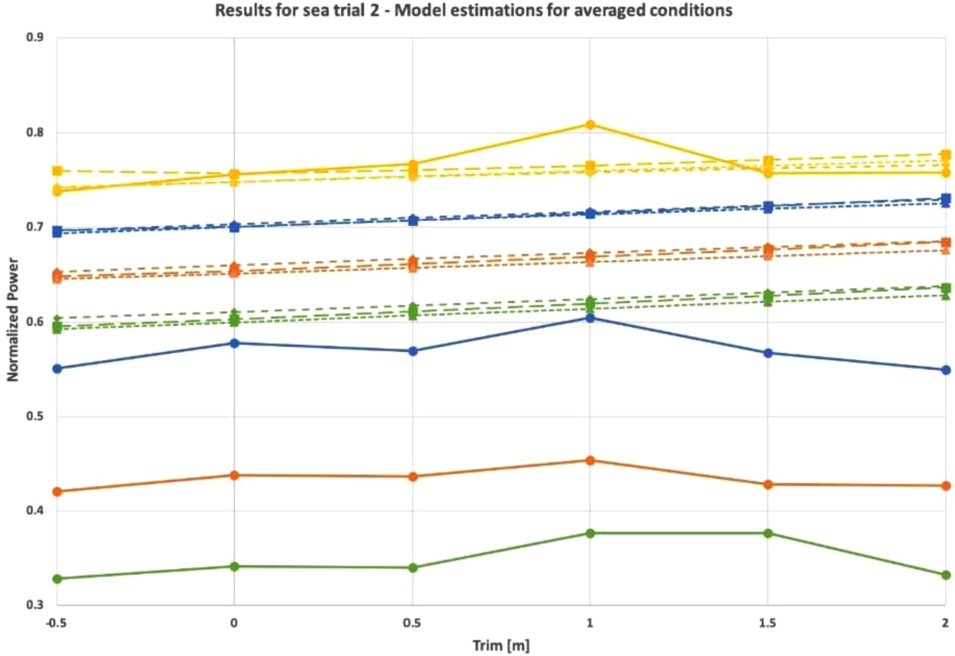
Model performance is validated in two ways. The first way is to copy all sea trial conditions one-to-one. The goal of this approach is to see how all effects, including the effect of weather and sea conditions, are embedded in the model and if the shaft power estimated by the model follows a similar curve as the shaft power from sea trial results. A drawback of this approach is that the actual effect of trim gets blurred by differences in external factors. For example, sea trial results may show a local maximum at a certain trim condition, but this may have been caused by an increase in wind. Therefore, the second approach is to take a considered average of the results of all conditions. The effect of trim only, provided by the model, can then be compared with the observed trend in the sea trial results. The results of both sea trials are shown in Figs 8–12.

Fig. 8.

Model- and sea trial results of the first sea trial in full load condition. Model input is equal to the actual sea trial conditions.

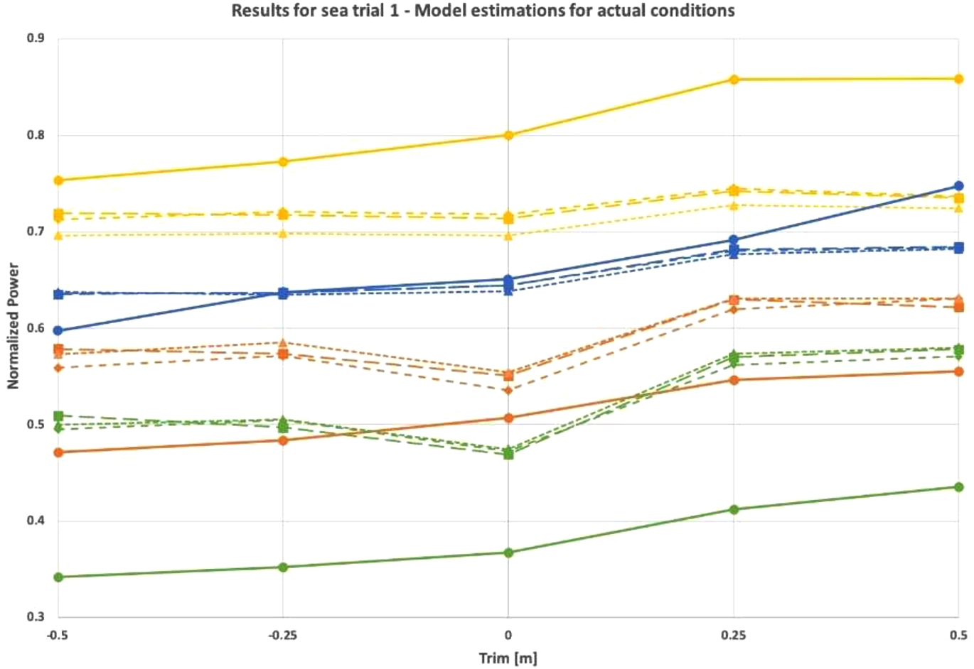
Fig. 9.

Model- and sea trial results of the first sea trial in full load condition. Model input is the average of the actual sea trial conditions.

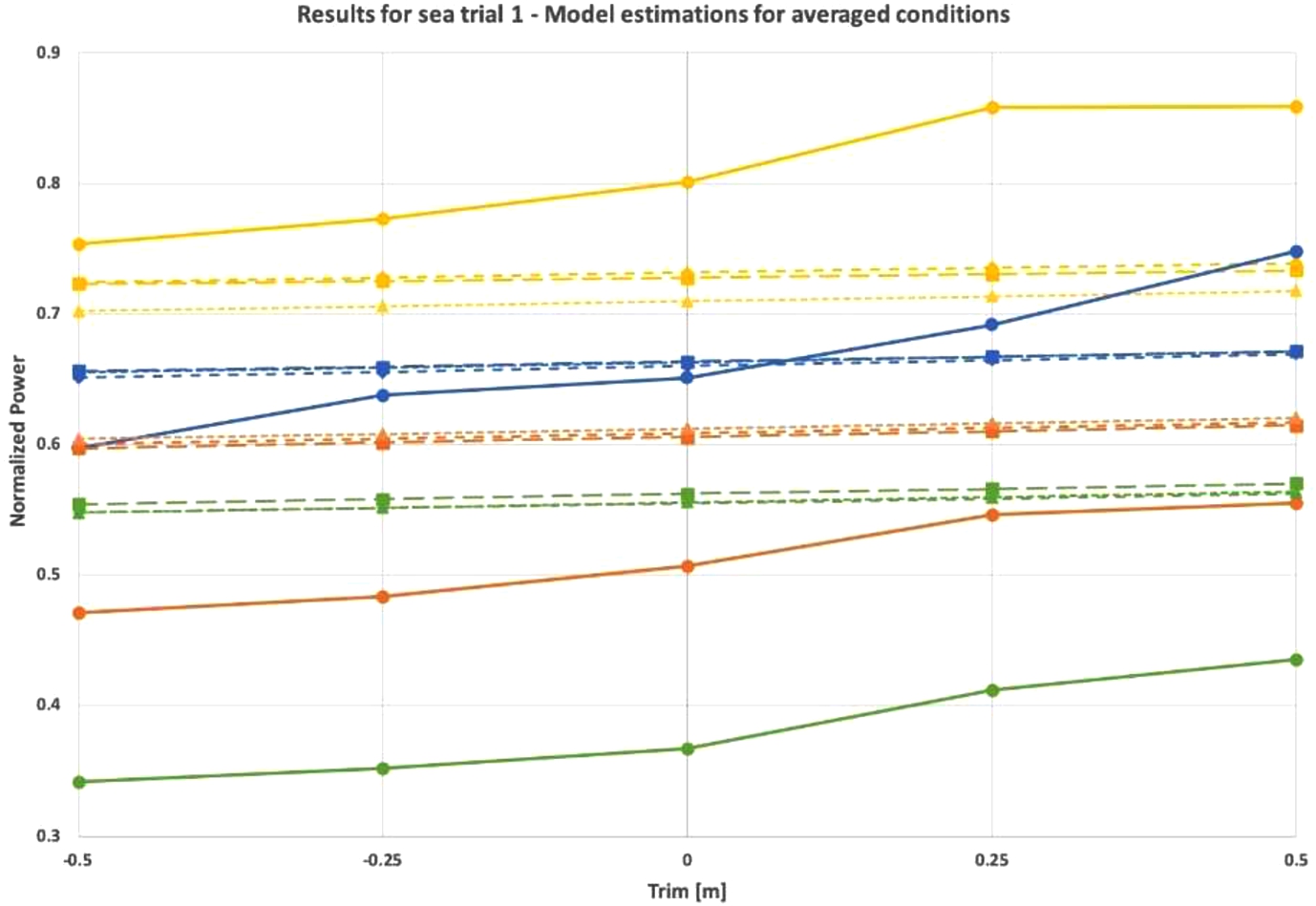
Fig. 10.

Model- and sea trial results of the second sea trial in ballast load condition. Model input is equal to the actual sea trial conditions.

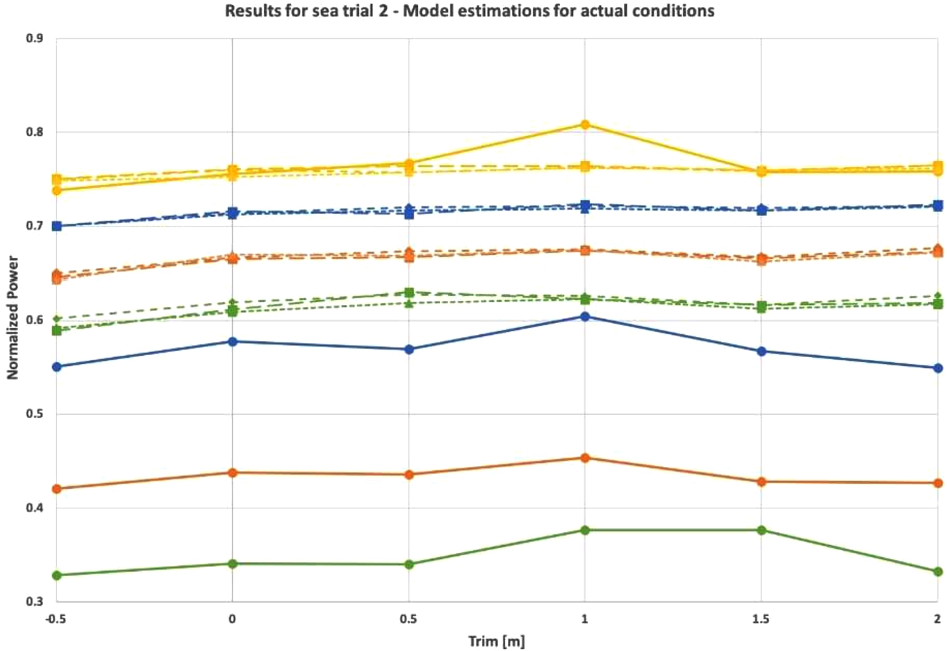
Fig. 11.

Model- and sea trial results of the second sea trial in ballast load condition. Model input is the average of the actual sea trial conditions.

Fig. 12.

Legend of Fig. 8–11.

6.2.1.Performance of model variants

The results of the model variant GBM-PLK and the pure BBM perform very similarly in both sea trial conditions. On a marginal level, the GBM-PLK shows a trend with a steeper slope for the first sea trial conditions, which is closer to the sea trial results than the trend of the BBM. Results of the GBM-PHM for the first sea trial show a weaker relationship between trim and power and for speeds of 11, 12 and 14 knots, an opposite trend is observed in the first sea trial.

6.2.2.Trend in trim on power

A clear trend is found in the results of the first sea trial, showing that an increase in trim causes an increase in required shaft power, despite the additional ballast water to achieve forward trim. Fuel model results show as well that the effect of trim is bigger than the effect of the small increase of mean draft due to additional ballast water (see Fig. 9). A similar trend with a smaller magnitude is found between trim and power by the fuel model. Regarding the first sea trial, on average a decrease in power of 1.3% is found when the ship is trimmed from even keel to 0.5 m bow trim. Sea trial results confirm that bow trim is optimal, with a similar trend, but with a much bigger magnitude. Depending on the speed, approximately 6% and 8% of required shaft power can be saved with a change in the trim of 0.50 m. The difference in power for stern trim conditions (stern trim of 0.25 m and 0.50 m) may be exaggerated, due to an increase in weather parameters. This increase is visible in the model output of Fig. 8 as well. A note should be made here that noon report data of negative trim was available but relatively very limited. This limits the model to accurately predict normalized shaft power for negative trim. Sea trial results with more positive trim would further allow evaluation of the model performance.

A much smaller effect of trim in power is found in the second sea trial. In zero noon reports, a stern trim of 0.25 m, even keel or bow trim for this load condition is recorded, meaning that the model is extrapolating for the data points of even keel and 0.5 m bow trim for this sea trial. For these conditions, propeller immergence cannot be ensured. The model nevertheless performs consistently with the sea trial results. The model performs worse compared to the first sea trial. A maximum is found for 1.0 m stern trim for speeds of 11, 12 and 13 knots and 1.0 m and 1.5 m stern trim for a speed of 11 knots. In the sea trial conditions, it is seen that the wind force was 5 Beaufort for this condition, instead of 3 or 4 Beaufort for other trim conditions. This peak in power is not as clearly visible in the model results. Also, the decrease in power visible in the sea trial results for a trim of 2.0 m is not seen in the model output. This local minimum is not visible in the trim tables based on model scale towing tests. A second sea trial can confirm if this local minimum is due to trim effects or other effects. Model results for a speed of 11 knots deviate the most, which is the speed represented by the least number of NR.

6.2.3.Structural deviations between fuel model and sea trial results

In the first sea trial, a local minimum in power is observed at even keel for speeds of 11 and 12 knots, which is not present in the sea trial results. This condition is specified with very calm water conditions with less displacement compared to the bow trim conditions, which could be a reason for this local minimum. Also, the clear drop of the sea trial results for a speed of 13 knots and a trim of −0.5 m in respect to −0.25 m, is not visible in the model results.

The trend between trim and power from the fuel model is similar for all mean drafts, whereas sea trial results and model scale towing tests show different magnitudes of the trend and a possible different trend for part load conditions. This indicates that the fuel model trend is averaged for all draft conditions, instead of a unique trend per draft condition. Since the majority of recorded draft conditions are for 9.5 m and more, it could be that the trend for this draft condition is (partly) extrapolated to other draft conditions. A solution could be to perform a model experiment, by training the neural network with noon reports for a limited range of draft conditions, for example, ballast load, part load and full load. Additionally, sea trials at part load conditions help to understand the effect of trim on power for this load condition.

Only a small difference in shaft power is seen between the trend lines of the model for different speeds, whereas the differences between the actual shaft power are much bigger. As was expected based on Fig. 7, weather factors dominate the power estimation, causing the effect of speed on shaft power is unrealistically embedded by the model, especially for moderate sailing conditions. For a full load condition, the model estimates the power correctly for a speed of 13 knots. For the part load condition in the second sea trial, the model estimates the power correctly for a speed of 14 knots. A few possible reasons can be given.

In the noon report data, a significant part of the lower speed recordings still have a high shaft power, explaining the weak correlation between speed and power found in the Spearman rank correlation analysis (see Fig. 4). Therefore, the achieved sailing speed is not only the result of the engine power but also of the weather and sea conditions, for which a similar shaft power is required.

The engine settings can be a reason as well for high shaft power at lower speeds. The considered ship class has a CPP with a shaft generator. To operate the shaft generator, a constant shaft speed is required, meaning that reducing sailing speed is to be done by decreasing the pitch only. This may cause a significant loss of the propeller efficiency, therefore (partly) explaining the higher recorded shaft power for lower speeds.

Errors in the noon report or sea trial data may cause errors in the model performance. These errors may include: (i) the mismatch between average shaft power and a snapshot of weather conditions and heading; and (ii) the human error in estimating and recording weather conditions and operational parameters (for example actual shaft power instead of day-average shaft power). From observing the NR data, it is known that draft and trim conditions are not always updated daily in the noon reports, while these are likely to change as a result of fuel consumption. Another reason for differences between model and sea trial results can be that the model does not include a parameter, which has a significant effect on shaft power or other input parameters.

6.2.4.Model applicability

Due to the cluster of recordings around a speed of 13 knots, the accuracy is optimal at around this speed and gets worse for speeds below 12 knots. A linear trend is found between trim and power for all mean drafts, showing potential in fuel savings between 1 and 2% for a change in the trim of 0.5 m. Validation with sea trials shows that the trend is fairly accurate for the full load condition and less accurate for the ballast condition. However, the magnitude of the trend is too small and the effect of speed on power is unrealistically embedded. Sea trials at ballast condition deviate for 1.0 m and more stern trim conditions with fuel model results.

Based on (i) the operational profile of the ship class, which shows that mean draft conditions bigger than 9.5 m represent 58% of the historical noon report data, (ii) the almost equal trend between trim and power in the fuel model against difference in magnitude of the power recording of the sea trial results and (iii) the possibility of a deviating trend at part load condition, it is concluded that the fuel model provides accurate trim advice for full load conditions. Despite the partially good performance of the fuel model for ballast condition, no sufficient evidence is provided yet that the fuel model should be used in practice for load conditions other than full load.

7.Discussion and modelling limitations

Model results regarding the trend between trim and power are now validated by two sea trials, each on a different mean draft condition. Some changes in shaft power in the performed sea trials are now attributed to external effects such as an increase in weather parameters. More sea trial results would enforce these statements. Sea trials are especially required to validate the model behaviour for part load conditions. Despite the promising initial results, the current model does have several limitations that should be addressed stemming, in part, from the noon report data source. Due to limitations in noon report data, it is not possible to capture all relevant parameters related to reducing shaft power, and thus this model cannot yet claim to be significantly (95%) exhaustive. While the Spearman Rank analysis provides confidence that vessel trim is one of the important variables that the ship operator can adjust, it cannot be said with certainty that it is the most significant factor. Other factors, such as propeller pitch of the CPP or detailed level of bio-fouling, are not captured but play a large role as well.

The extracted trends between trim and required shaft power are almost equal for all draft conditions. Considering the robust design of the ship in the case study, this might be true. However, sea trial results indicate a different magnitude of the effect of trim for different draft conditions. Moreover, the results from model scale towing tests indicate a different trend for a mean draft of 7.0 m, which is not yet validated by sea trials. It cannot be concluded with confidence that the extracted trends by the fuel model are true for all mean drafts. A possible solution would be to group the noon reports for different draft conditions and perform the analysis presented in the report for each group of mean drafts. The result would be a trend between trim and power for each group of the mean draft, which would increase the interpretability of the GBM and enable to conclude if different trends exist for different groups of mean drafts. Since the number of noon reports will be less for each group of mean drafts, the number of groups of drafts should be limited.

Power estimations of the WBM deviate significantly from the power recordings in the noon report data for speeds below 12 knots and above 14 knots. A research opportunity is identified, to research the effect of a modified WBM on the performance of the GBM. The WBM modification can be done by including an estimation of the effect of weather conditions on the required shaft power in the WBM, which could improve the extrapolation qualities of the GBM. The model accuracy would then improve for speeds outside the region of 12 to 14 knots of speed.

The specific fuel consumption (sfc) is assumed to be constant. However, this will be a function of engine speed, pitch setting of the CPP, and maintenance level and will differ between ships. To estimate the fuel consumption more accurately, this assumption should be dropped and be determined as a function of the mentioned factors.

The effect of hull and propeller fouling is included by considering only the days since the last hull cleaning and last propeller polishing. However, the actual degree of fouling is much more complex. Further model improvements may consider for example the geographical locations or the consecutive days in warm water.

8.Conclusion

The GBM-PLK variant is considered to perform superior to the other model variants. This model followed the trend of the sea trial results the most accurate. The accuracy of the GBM-PLK fuel model is 6.58% for a random test subset from the noon report data, which was slightly better than the other model variants. The GBM-PHM variant has shown to result in opposite relations between trim and power compared to the results of the sea trials in multiple cases. A linear trend is found between trim and power for all mean drafts, showing potential in fuel savings between 1 and 2% for a change in trim of 0.5 m.

Validation by sea trials has shown that the model is able to provide correct trim advice, while considering dynamic effects of weather and sea conditions, for full load conditions and speeds between 12 and 14 knots. These conditions are most frequently encountered in the NR data. The effect of speed on power is unrealistically embedded in the model for other conditions than calm water.

The data pre-processing framework has been constructed and used successfully for this case study. However, due to the nature of noon reports, the quality of the noon report data remains a source of noise. As a consequence, the knowledge that can be extracted from noon report data remains to find trends, but the magnitude is likely to differ from the actual effects. The main problems with using noon report data are:

The discrepancy between the averaged recordings of shaft power and speed through water over 24 hours on one hand, and the snapshot of weather and sea conditions and the relative direction on the other;
the highly concentrated power recordings for a certain engine setting, causing weakly defined relations between speed and power;
accurate and daily updated static forward and aft draft is a prerequisite to finding realistic trends between trim and required power.

No indication is observed showing that the GBM approach increases the extrapolation qualities of the BBM, nor decreases it. The most significant limitation in input data is the relatively small number of noon reports with small forward draft conditions (small mean draft with forward or even keel trim condition) and low speed (lower than 11 knots) recordings. The effect of speed on power is not realistic for both the GBM and the BBM approach and no difference is observed between the model variants in low forward draft conditions. Other advantages of a GBM over a pure BBM may still hold, which have not been proven in this analysis. These advantages include the prevention of unreasonable results, and the possibility to use less historical data than a pure BBM.

Acknowledgements

This work was performed as part of the MSc thesis for the lead author, Robert Zwart [29]. The thesis was performed in Marine Technology at Delft University of Technology in collaboration with Stolt Tankers. The authors would like to acknowledge both Delft University of Technology and Stolt Tankers for their support of this research.

Funding: The authors report no funding.

Conflict of Interest: The authors have no conflict of interest to report. Austin A. Kana is an Editorial Board Member of this journal, but was not involved in the peer-review process nor had access to any information regarding its peer-review.

Author Contributions: Robert Zwart: Conception; performance of work, interpretation of data; writing of the article. Jordi Bogaard: conception; interpretation of data; writing – review and editing. Austin A. Kana: Conception; interpretation of data; writing of the article.

References

[1]	A.H. Abouedafdl and E.E.Y. Abdelraouf, The impact of optimizing trim on reducing fuel consumption, Journal of shipping and Ocean Engineering 6: ((2016) ), 179–184. doi:10.17265/2159-5879/2016.03.006.
[2]	L. Aldous, T. Smith and R. Bucknall, Noon report data uncertainty, in: Low Carbon Shipping Conference, London, (2013) .
[3]	E. Bal Beşikçi, O. Arslan, O. Turan and Ölçer, An artificial neural network based decision support system for energy efficient ship operations, Computers and Operations Research 66: ((2016) ), 383–401. doi:10.1016/j.cor.2015.04.004.
[4]	A. Coraddu, L. Oneto, F. Baldi and D. Anguita, Vessels fuel consumption forecast and trim optimisation: A data analytics perspective, Ocean Engineering 130: ((2017) ), 351–370. doi:10.1016/j.oceaneng.2016.11.058.
[5]	Da Silva et al., Artificial Neural Networks – a Practical Course, 1st edn, Springer International Publishing, (2017) .
[6]	DNV-GL, ECO assistant 4.1. 2013. Available from: http://production.presstogo.com/fileroot7/gallery/DNVGL/files/original/6a40ec4017884ae99d8c1ac206de8f96.pdf [cited 28 October 2019].
[7]	Y. Du, Q. Meng, S. Wang and H. Kuang, Two-phase optimal solutions for ship speed and trim optimization over a voyage using voyage report data, Transportation Research Part B 122: ((2019) ), 88–114. doi:10.1016/j.trb.2019.02.004.
[8]	M.R. Forster, Notice: No free lunches for anyone, Bayesians included, Department of Philosophy, University of Wisconsin Madison, Madison, USA, 2005.
[9]	X. Gao, K. Sun, S. Shi, B. Wu and Z. Zuo, Research on the influence of trim on a container ship’s resistance performance, in: 3rd International Conference on Fluid Mechanics and Industrial Applications, Taiyuan, China, June 29–30, (2019) .
[10]	A. Garcia, S. Ramírez-Gallego, J. Luengo, J.M. Benítez and F. Herrera, Big data preprocessing: Methods and prospects, Big Data Analytics 2016: (1) ((2016) ), 9. doi:10.1186/s41044-016-0014-0.
[11]	J. Holtrop and G.G.J. Mennen, An approximate power prediction method, International Shipbuilding Progress 29: ((1982) ), 166–170. doi:10.3233/ISP-1982-2933501.
[12]	IMO, Guidelines for voluntary use of the ship energy efficiency operational indicator (EEOI). MEPC.1/Circ.684, 2009.
[13]	IMO, Low carbon shipping and air pollution control, 2019. Available from: http://www.imo.org/en/MediaCentre/HotTopics/GHG/Pages/default.aspx [cited 25 December 2019].
[14]	H. Islam and C. Guedes Soares, Effect of trim on container ship resistance at different ship speeds and drafts, Ocean Engineering 183: ((2019) ), 106–115. doi:10.1016/j.oceaneng.2019.03.058.
[15]	L.P. Leifsson, H. Sævarsdóttir, S. Sigurđsson and A. Vésteinsson, Grey-box modeling of an ocean vessel for operational optimization, Simulation Modelling Practice and Theory 16: ((2008) ), 923–932. doi:10.1016/j.simpat.2008.03.006.
[16]	M. Lutzen and H.O. Kristensen, Prediction of resistance and propulsion power of ships, 2013. Available from: https://www.danishshipping.dk/en/services/beregningsvaerktoejer/download/Basic_Model_Linkarea_Link/163/wp-2-report-4-resistance-andpropulsion-power.pdf [cited 18 November 2019].
[17]	MEPC, Energy efficiency technologies information portal, No date. Available from: https://glomeep.imo.org/resources/energy-efficiencytechologies-information-portal/ [cited 17 October 2019].
[18]	A.I. Parkes, A.J. Sobey and D.A. Hudson, Physics-based shaft power prediction for large merchant ships using neural networks, Ocean Engineering 166: ((2018) ), 92–104. doi:10.1016/j.oceaneng.2018.07.060.
[19]	B.P. Pedersen and J. Larsen, Prediction of full-scale propulsion power using artificial neural networks, in: Proceedings of the 8th International Conference on Computer and IT Applications in the Maritime Industries, Budapest, Hungary, (2009) , pp. 537–550.
[20]	B.P. Pedersen and J. Larsen, Gaussian process regression for vessel performance monitoring, in: 12th International Conference on Computer and IT Applications in the Maritime Industries (COMPIT 13), Cortona, Italy, (2013) .
[21]	J.P. Petersen, D.J. Jacobsen and O. Winther, Statistical modelling for ship propulsion efficiency, Journal of Marine Science and Technology 17: ((2012) ), 30–39. doi:10.1007/s00773-011-0151-0.
[22]	A. Radonjic and K. Vukadinovic, Application of ensemble neural networks to prediction of towboat shaft power, Journal or Marine Science and Technology 20: ((2015) ), 64–80. doi:10.1007/s00773-014-0273-2.
[23]	United Nations, The Paris agreement, 2015. Available from: https://unfccc.int/process-and-meetings/the-parisagreement/the-paris-agreement [Cited 25 December 2019].
[24]	E. Van Ballegooijen, T. Helsloot and M. Timmer, Experience with full-scale thrust measurements in dynamic trim optimisation, in: 3rd Hull Performance and Insight Conference, Redworth, England, 12–14 March, V. Bertram, ed., (2018) , paper no. 5, pp. 36–47.
[25]	D.H. Wolpert, The lack of a priori distinctions between learning algorithms, Neural Computation 8: (7) ((1996) ), 1341–1390. doi:10.1162/neco.1996.8.7.1341.
[26]	Yang et al., A genetic algorithm-based grey-box model for ship fuel consumption prediction towards sustainable shipping, Annals of Operations Research ((2019) ), 1–27. doi:10.1007/s10479-019-03183-5.
[27]	J. Yuan and V. Nian, Ship energy consumption prediction with Gaussian process metamodel, Energy Procedia 152: ((2018) ), 655–660. doi:10.1016/j.egypro.2018.09.226.
[28]	P. Zhang, Advanced Industrial Control Technology, 1st edn, Elsevier Inc., Oxford, (2010) .
[29]	R.H. Zwart, Trim optimization for ships in service: A grey-box model approach using operational voyage data, MSc Thesis, Delft University of Technology, 2020.