A reduced order model for FSI of tank walls subject to wave impacts during sloshing

Bos, R.W.; van der Eijk, M.; den Besten, J.H.; Wellens, P.R.

doi:10.3233/ISP-220003

A reduced order model for FSI of tank walls subject to wave impacts during sloshing

Article type: Research Article

Authors: Bos, R.W. | van der Eijk, M. | den Besten, J.H. | Wellens, P.R.^{; *}

Affiliations: Department of Maritime and Transport Technology, Delft University of Technology, Netherlands

Correspondence: [*] Corresponding author. E-mail: p.r.wellens@tudelft.nl.

Keywords: Fluid-structure interaction, sloshing, dynamics, non-hydrostatic shallow water equations, wave impact

DOI: 10.3233/ISP-220003

Journal: International Shipbuilding Progress, vol. 69, no. 2, pp. 119-138, 2022

Received 21 February 2022

Revision received 2 October 2022

Accepted 28 October 2022

Published: 7 December 2022

Get PDF

Abstract

Loads due to wave impacts are a limiting factor in the design of liquefied natural gas (LNG) tankers and their insulation. The current methodology considers the load independent from the response of the tank. Better tanks can be designed by knowing the effect of the interaction between the wave loads and the response, however predicting these effects is computationally expensive. In this paper a new application of the non-hydrostatic shallow water equations are presented, namely as a reduced order model (ROM) for fluid structure interaction for wave impacts. Our ROM is compared to a high fidelity model. The proposed ROM is fast and accurately predicts the total impulse and added mass, and therefore the general behaviour of the structure during the free vibration phase. It does however not always accurately predict the maximum force. It is therefore considered an appropriate tool for a first screening of the loads for which fluid-structure interaction is important, after which a more accurate method can be used to evaluate the most interesting cases. A sensitivity study is performed for various impact angles and velocities, showing that the importance of fluid structure interaction depends highly on the specific situation.

Wave impacts on inner walls are known phenomena in liquefied natural gas (LNG) sloshing on board of LNG tankers, and is characterized by high variability of the loads due to free surface instabilities before impact [2]. The LNG in the tanks is kept at its boiling point (−162°C), causing phase change in the liquid and cryogenic temperatures for the tank walls which should maintain structural integrity at all times. An insulating cargo containment system (CCS) is applied to the tank walls in order to prevent the steel hull from becoming brittle. For an optimal insulation the tank walls should be as light and thick as possible, for maximum strength they should be as thin and heavy as possible. These contradicting requirements combined with the variability of loads complicate the design of such a CCS.

The design loads of a CCS are typically determined using model tests on a 1:40 scale [11]. A rigid scale model of the LNG tank is fitted with pressure sensors and excited in a similar way as the real tank would. The pressures are statistically post-processed and applied to the structure in patches [21]. In this approach the dynamics and flexibility of the structure is not directly taken into account, only through dynamic amplification factors.

A large test campaign investigating wave impacts for LNG CCS is the ‘Sloshel’ project [2,3,15]. A full scale LNG CCS was placed in a vertical end wall of a flume. Then different shapes of waves loading the wall were obtained by changing positions of the focal point with respect to the wall. Depending on the wave shape, three elementary loading processes (ELPs) were identified [17]:

1. Direct impact: the first part of the wave hits the wall, and liquid compressibility is important
2. Building jet: the fluid has to change direction and spreads along the wall
3. Pulsating gas pocket: enclosed gas is compressed and causes a varying load

Each of these ELP’s has a different signature, physics, and scaling [8], which makes the aforementioned model tests difficult to translate to real tank applications. However, not all these ELP’s are of equal importance for the response of the structure. The response depends on the loaded area and time signature, as for instance demonstrated in [5]. Furthermore, if it is known which loads (or ELPs) are most important for the structural response, then the hydrodynamicist can focus on accurately predicting these loads.

Fig. 1.

The Mark III cargo containment system as designed by GTT. Drawing and dimensions similar to [12,16].

The structure considered in this paper is the ‘Mark III’ CCS of the company GTT [10,13], which is a sandwich structure with a foam core and plywood face sheets, a cross-section is shown in Fig. 1. On the inside of the tank a stainless steel membrane is fitted to keep the LNG inside, and a secondary membrane is fitted between the foam layers for redundancy. In order to minimize thermal stresses, relaxation grooves are cut just above the secondary membrane, creating ‘subpanels’ of 340 by 340 mm which are to a large extent uncoupled [4]. Note that Fig. 1 represents a slice of the subpanel.

The CCS has two main failure modes: plastic indentation failure of the foam and shear failure of the bottom plywood [6,13]. If either of these two failure modes occur, then there is a high probability that also one of the membranes will fail, which is to be avoided at all times. A reduced order model for the onset on indentation failure is presented in [4], based on [20] and [24]. Prediction of the structural response can be significantly sped up using such a reduced order model, possibly leading to great simplification of the coupled problem.

The problem is however slightly more complex, as shown for instance in [18], where sloshing model tests including FSI are described for a flip-through impact. A 2D tank is used with an elastic flat wall at the end, which represents the CCS. The deformations of the wall are measured and computed (using pressures on the rigid wall). A comparison shows that the wall response requires more than just the pressure on the wall and added mass and damping, especially due to the change of added mass in time. This means for us that the response of the structure to the loads (one way coupling) is different from the fully coupled response (two way coupling). Hence, it can be necessary to take the two way coupling between the load and wall into account when investigating which loads are important.

The two-way coupling can be investigated for the entire tank, as demonstrated in [28]. Here the stiffness of the wall was varied and the tank excited in the same way. As the tank wall becomes increasingly compliant, the pressures decrease and show a more vibratory response. The total time during which the pressure sensor was loaded is longer. This is however numerically expensive and time consuming, especially considering the highly variable loads that require a probabilistic assessment.

For such a probabilistic assessment we look at simplified models, that are fast and sufficiently accurate for the situations in which they are used. The load due to a wave impact and therein encapsulated air can be predicted using two simplified models: the Wagner and Bagnold model [19]. First, the Wagner model can describe the building jet (ELP2) based on an initial shape and potential theory for the flow [25]. The load of the Wagner model starts with a high pressure peak and very locally, then spreading out and then spreads out over the wall while the total force increases. Second, the Bagnold model describes how entrapped gas pulsates (ELP3) based on a gas law and some moving mass representing the surrounding water [1].

In this paper the coupling between the CCS and a wave impact is investigated on the subpanel level. The subpanel is represented by the beam-foundation model proposed in [4], which predicts the response to the first vibration mode of the CCS. ELP 2: ‘building jet’ is chosen as load case, because it is expected to give a response on the length and time scale as the structure. This paper focusses on how the load is modelled and how the load interacts with the structure. It presents a simplified model for ELP2, in the form of non hydrostatic shallow water equations (NHSWE [14]), made suitable for numerical implementation of the coupling. To our knowledge this is the first paper to propose a reduced order model for fluid-structure interaction for wave impacts, that is fast and versatile enough for probabilistic evaluation. Figure 2 shows how the reduced order model from this paper relates to an actual wave impact. The drawn lines approximate the shape of the breaking wave, symmetrical over the horizontal plane. We developed this model to be faster than a high fidelity CFD code, so that it can be used in to perform a sensitivity study of the importance of FSI for various wave impact parameters.

Fig. 2.

Wave impact from [17]. The orange lines represent the cut-off wedge impact which is simulated in this paper. The cut-off wedge has an initial constant velocity v0 towards the wall, an angle α and an initial height h0.

In the rest of the paper we will derive the equations for the fluid model and couple it to the structure. Then a number of wave impact scenarios are investigated with this code and a more detailed in-house CFD code: EVA. EVA is based on the Navier–Stokes equations for the motion of a mixed fluid with varying properties to model the combination of a liquid and a gas phase. The robust method makes use of a fixed staggered Cartesian grid where for the convective term a second-order upwind scheme is used. The time integration is based on a second-order Adams–Bashforth scheme. The description of the free surface is done with the Volume-of-Fluid (VoF) where the interface is geometrically reconstructed using piecewise-linear line segments. Free surface waves can be generated at boundaries, while reflected waves from the inside of the domain can be absorbed at the same time [26]. By consistently coupling the mass and momentum fluxes, EVA is capable to model high density ratio two-phase flows. The externally added interaction is solved using the Crank Nicolson scheme in the reduced order model and in EVA. A detailed description and validation of the CFD flow solver EVA is given in [23]. Both codes are used in this paper to investigate the effects of fluid-structure interaction for a wave impact.

1.Method

The starting point is the Wagner impact model, which assumes an initial shape and constant velocity. It then calculates the flow and wall pressures using some perturbation method [19]. However, such a solution may not be feasible for the coupled problem, in which the relative velocity between structure and fluid is not constant. By making the following assumptions we have a similar starting conditions but obtain a model which is easier to solve. The following is assumed:

The wave impacts are perpendicular to the wall, and are symmetric with respect to the axis normal to the wall.
Water height and velocity are prescribed along the normal of the wall, and are only a function of the distance to the wall.
Gravity and air are disregarded in the solution, but kept in the derivation to be in line with literature

With these assumptions we obtain the non-hydrostatic shallow water equations [14,22,27]. In these equations part of the pressure is caused by the vertical acceleration of the fluid. Therefore the assumption of Wagner, disregarding gravity for an impact, can be used, and comparison is possible.

1.1.Fluid equations of motion

A similar approach is taken to derive the fluid equations as in [14], only here a flat bottom is assumed representing the symmetry of the impact. The starting point of the Fluid model are the Euler equations:

(1)u,x+w,z=0Continuity(2)u,t+uu,x+wu,z=−p,x/ρMomentum x(3)w,t+uw,x+ww,z=−(g+p,z/ρ)Momentum z

where u,w are the velocity fields in x,z direction, and u,x denotes the derivative of u to x. The kinematics are defined as:

(4)u=U,w=zH˙H

where H is the free surface level and H˙=H,t+uH,x. Therefore the velocity field of w interpolates the velocity at the free surface to a point in between. Instead of having to define u,w over the complete fluid domain we now only have to define it over the x axis, hence the problem is reduced from two dimensional to one dimensional. In order to solve the equations of motion we need to loose the z that appears in all equations due to w. Therefore we integrate all equations over the height, which is similar to using the method of weighted residuals in one direction [9]. The height averaged vertical velocity is:

(5)W=1H∫0Hwdz=1H∫0HzH˙Hdz=12H˙

We can now average the continuity equation over the height:

(6)0=∫0Hu,x+w,zdz=H˙+HU,x(7)=H,t+(UH),x

and momentum x equation:

(8)∫0Hu,t+uu,x+wu,zdz=∫0H−p,x/ρdz(9)H(U,t+UU,x)=−f,x/ρwith f=∫0Hpdz

Note that in the latter, the atmospheric pressure is equal to zero. Equation (3) can be simplified, by substituting the kinematics:

(10)−(g+p,z/ρ)=w,t+uw,x+ww,z(11)=z(H˙H·_+H˙2H2)(12)=z(H¨H−H˙2H2+H˙2H2)(13)=zH¨H

This equation can be further simplified, by weighing with z and integrating over the height. We weigh with z in order to end up with the average wall force f at the left hand side.

(14)∫0H−z(g+p,z/ρ)dz=∫0Hz2H¨Hdz(15)−12gH2−[zp]0H/ρ+∫0Hp/ρdz=∫0Hz2dzH¨H(16)−12gH2+f/ρ=13H2H¨

Here we could use the assumption that H¨ is small leads to the shallow water equations. However, we substitute the definition of W into this equation of motion, giving:

(17)−12gH2+f/ρ=23H2W˙

To summarize, we have the following equations that describe the fluid behavior:

H,t+(UH),x=0ρH(U,t+UU,x)=−f,xρ23H2W˙=−12ρgH2+fH˙=2W

1.2.Implementation

The fluid model is discretized with a fractional step method. The first step, from tn to t∗ is pure convection, all right hand side is at tn:

(18)H∗−HnΔt=−HU,x−UH,x(19)U∗−UnΔt=−1ρHf,x−UU,x(20)W∗−WnΔt=32ρH2f−UW,x

The second step is to proceed from t∗ to tn+1, while enforcing the incompressibility condition and boundary conditions. It is assumed the wave height is not changing in the second step:

(21)Hn+1=H∗(22)ρHUn+1−U∗Δt=−f,xc(23)23ρH2Wn+1−W∗Δt=(fc−12gH2)(24)0=2Wn+1+H∗U,xn+1

where fc is a pressure correction, used to enforce continuity. The boundary conditions are added here and the linear system is solved for the new time step tn+1. The last step is to correct the pressure:

(25)fn+1=fn+fc

Equations (22)–(24) can be combined to yield an equation for fc. First, Equations (22) and (23) are rewritten for Un+1 and Wn+1. This is then submitted into Equation (24), giving the following equation:

(26)ρΔt(2W∗+HU,x)∗−32g=31H2f+H,xHf,x−f,xx

To solve the system we need boundary conditions which are on the velocity, not on the pressure. Therefore the system is transformed to have on the boundaries the first derivative of the pressure as unknown. It allows us to prescribe the change in velocity that the pressure correction needs to deliver.

The equations are solved using collocated vertex centered finite differences. Discretization is upwind for convective terms, and central for the terms in Equation (26). The vertices are spaced evenly, dividing the L=1 m domain into 250 parts of equal length.

1.3.Structure equations of motion

The CSS is simplified to a mass-spring system following [4], giving an equation of the following form:

(27)ms¨+cs˙+ks=f

with s=s(t) as displacement, mass m, damping c, stiffness k and external force f. The equations of motion are converted to state space form (u˙(t)=Au(t)+h(t)) and integrated over time using Crank–Nicolson:

(28)u1=u0+12(Au1+h1+Au0+h0)Δt(29)A=01−k/m−c/m,u=ss˙,h=0f/m,

where subscript 1 denotes the new state and 0 the old state, matrix A describes the system dynamics, h(t) is the external load and u(t) the state of the system. This method is chosen because it is stable and conservative.

1.4.Coupled solution

The structure is placed at the edge of the fluid domain x=L. For the wave impact problems investigated here, we assume the deformations of the structure are small, so that we need not modify the fluid domain. The inflow / outflow velocity of the fluid is made equal to the velocity of the structure: U(x=L,t)=s˙(t). The force on the structure is equal to the force on the wall of the fluid: Q(x=L,t)=f(t).

The actual coupling takes place in the pressure correction step of the fluid. The structure is added to the system of equations of the fluid, thus solving both at the same time. This avoids sub-iterations or the choice of under relaxation parameters required for a partitioned solver and gives a robust implementation. The resulting system of equations is directly solved without iterations.

2.Uncoupled wedge impact

Following the initial investigation of the governing equations, a number of important parameters can be deduced. First, the rise time of the load. At the start the change from wedge to rectangle is at xc=h0/tanα. The starting velocity is v0, so if the cut-off wedge would move along with the flow, the arrival at the wall would be:

(30)tc=xcv0=h0v0tanα

After this critical time tc the force on the wall should go from wedge-dominated to rectangle-dominated. Second, we investigate the load level. If an infinite wedge impact on a wall is investigated with the Wagner model, the force would be [29]:

(31)F(t)=C(α)ρv03t

where C(α) is a constant depending on the wedge angle, v0 the velocity at far field and t the time. On the other hand, if there was only water being bent off by the wall, conservation of momentum would give:

(32)F(t)=ρh0v02

In the worst case scenario the wedge behavior will continue up to tc, giving the maximum force:

(33)Tmax=C(α)ρv02h0tanα

To better compare the results we decide to present them in a dimensionless form, when applicable. The dimensionless time τ and force ϕ are defined as:

(34)τ=tv0tanαh0,ϕ=Fρh0v02

Here we choose to make the force dimensionless by the steady state force on the wall instead of the peak force, because the former does not depend on the impact angle. Additionally we make the time dimensionless using the critical time. All calculations are performed with water density ρ=1000 kg/m³, an initial height h0=0.2 m.

Due to the assumptions made in modelling the fluid flow there is no straightforward validation problem. However, we believe that the comparison between the reduced order model and EVA give enough confidence to trust this method for optimization or probabilistic evaluations. Because EVA is validated for fluid flow it is possible to make the link with reality. Additionally, this model is meant to predict the relevant trends, and the effect of taking hydro-elasticity into account. The next step could be to extend the model in a way that allows direct comparison with experiments.

Fig. 3.

Dimensionless plot of grid convergence of force on the wall for the two impact angles for EVA.

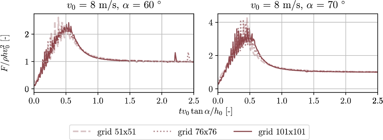
A convergence study for EVA for the investigated wedge angles is shown in Fig. 3. This figure shows on the horizontal axis dimensionless time and vertical axis the dimensionless total force on the wall. The dimensionless force on the wall is shown to converge to a constant value. The irregularity in the force just after impact, before the force starts to converge, is due to the dynamics of the liquid. Each time a cell originally filled with gas becomes filled with liquid it leads to a label change of that cell and some irregularity in the pressure. Such a label change is also visible near dimensionless time 2.2 for one grid and at time 2.4 for another (α=60∘, graph on the left). In this paper all calculations are performed on a 1 by 1 m grid, with water (ρ=1000 kg/m³) and ‘air’ (ρ=1e-8 kg/m³). The air density is chosen to be close to zero, which matters for the comparison with the NHSWE code in which there is no air. The grid resolution as varied between 51, 76 and 101 cells in each direction on a Cartesian grid, which are the values 51 × 51 and so forth in Fig. 3. At the same time the time step was appropriately scaled by enforcing CFL <0.1 at all times. The wall force is roughly the same for all grid resolutions, however the noise decreases when the grid is more refined. The noisy behavior, is caused by local pressure spikes. These are caused by the correction to the explicit momentum terms to remain divergence free and is associated with the large density ratio. For the fully coupled scheme, Crank Nicolson is used which relaxes these local pressures.

Fig. 4.

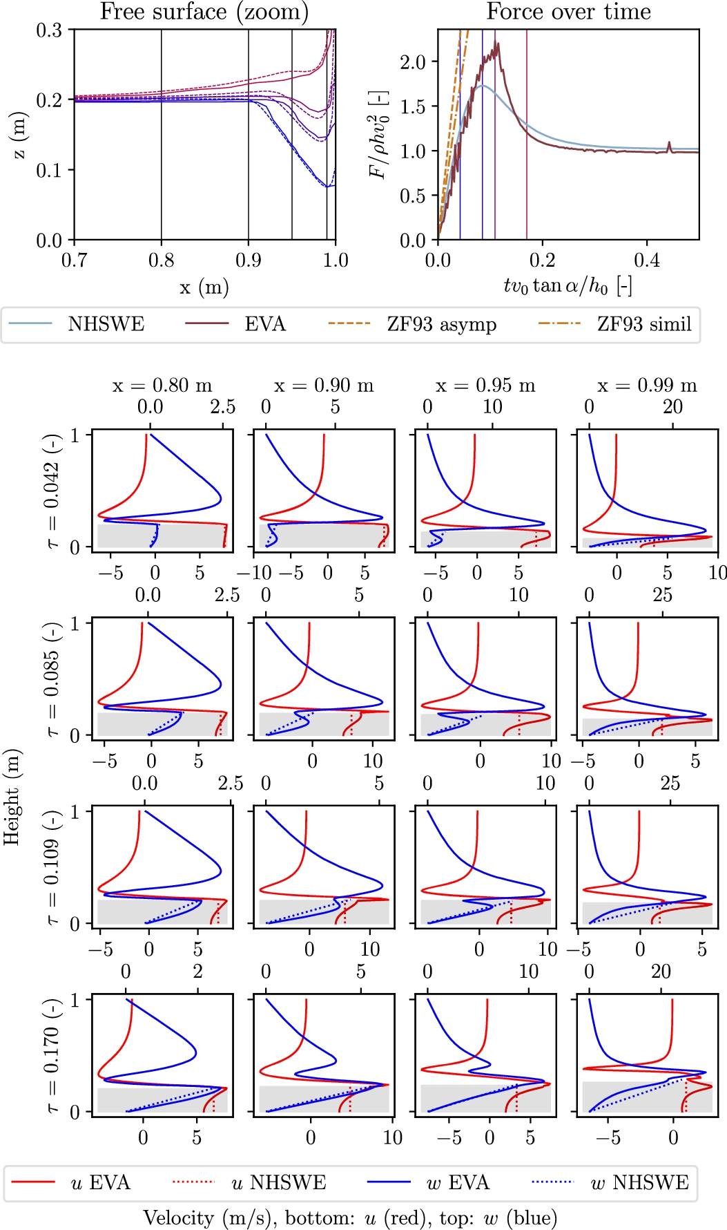
Top row shows the free surface over time, as well as dimensionless force over time. The matrix below gives velocity over height for impact with v0=8 m/s and α=60∘. The rows are different dimensionless times, the columns are positions in front of the wall.

Fig. 5.

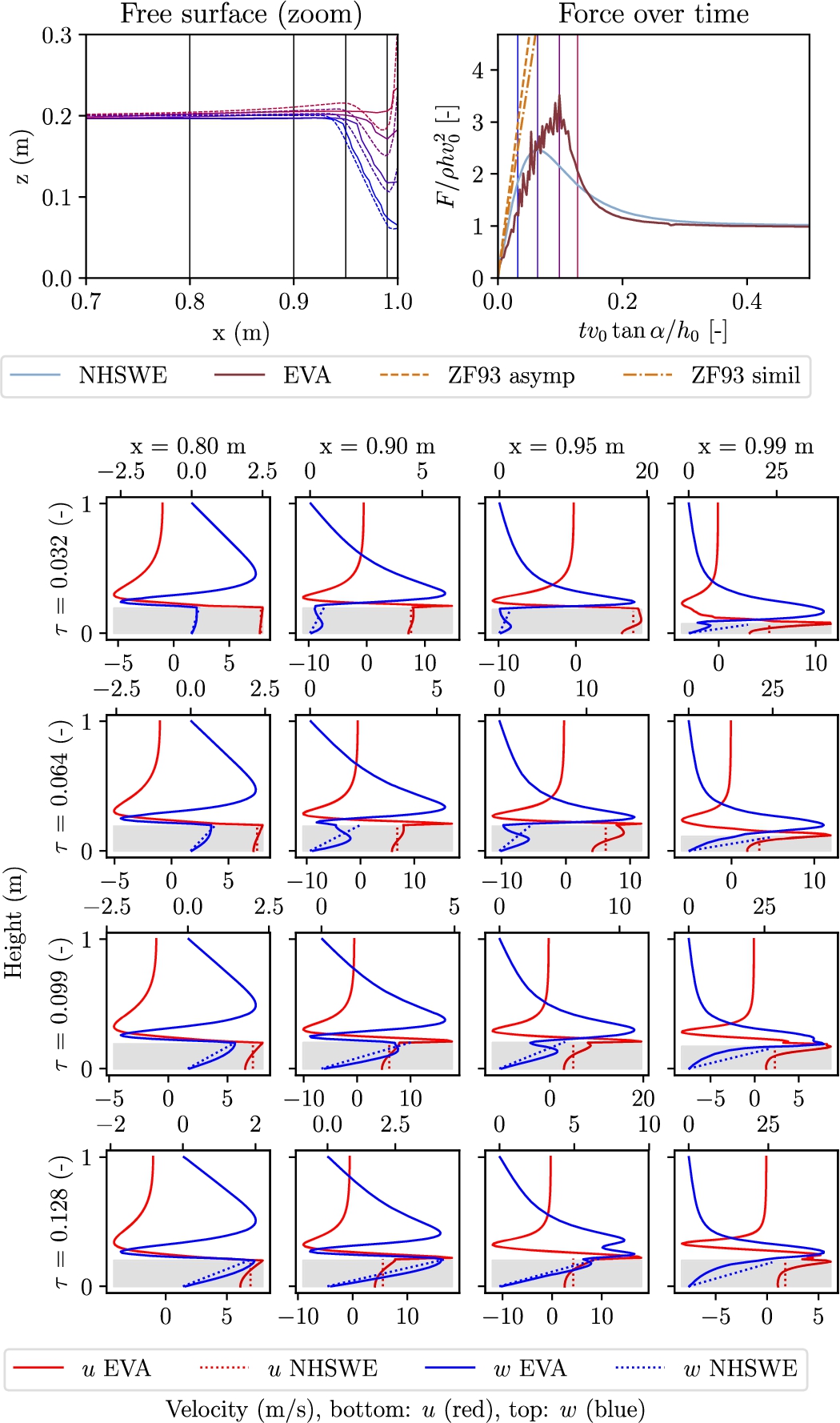
Top row shows the free surface over time, as well as dimensionless force over time. The matrix below gives velocity over height for impact with v0=8 m/s and α=70∘. The rows are different dimensionless times, the columns are positions in front of the wall.

Figures 4 and 5 show the force on the wall for an impact with v0=8 m/s with α= 60° and 70°. These impact velocities and angles are chosen because they have the impact duration that causes hydro-elasticity to have an effect, other angles are shown later in Fig. 7. First the impact force follows the result of [29], as shown by the two lines indicating ‘ZF93’. They are analytical Wagner solutions to the impact problem, and the numerical result should be similar during the first part of the impact. Although for the wedge water entry case [29] and the plate wedge water impact case (Figs 4 and 5), the roles of the fluid and the structure are reversed. For wedge water entry the body is penetrating the flat fluid surface and for plate wedge water impact a wedge shaped fluid surface is impacting a flat body – the way the impact force develops is similar [8].

Both codes, NHSWE and EVA, adhere quite well to the expected rate at which the force builds up. At some point the slope decreases and the maximum force is reached and this depends highly on the angle α as mentioned before. Finally, all scaled impact forces converge to unity as expected. If the actual Wagner model was used, the load would keep on rising indefinitely, as in that case there is no end to the wedge. These tests have been repeated using different impact velocities but yield the same curve, meaning our aforementioned scaling factors work. It is clear that EVA shows a much higher peak value, up to 40%. Even disregarding the spikes in the force of EVA, likely caused by the fluid going into the next cell, the maximum force is about 30% higher. However, it should be noted that the difference in total impulse is within 3% percent because the same mass of fluid has to be turned around. In order to explain why there is a difference in maximum force, we need to look at the velocity profiles.

We know that there is one big difference between the models: EVA has multiple cells over the height of the domain, whereas NHSWE has only one. This allows EVA to have more local details, which we know the wave impact problem has [7,25]. The different velocity fields at four places are plotted in Figs 4 and 5, for four times (before max, max NHSWE, max EVA and near steady). These positions and times are indicated in the free surface and force over time plots in these Figures. In the second row of Figs 4 and 5 we can observe why the peak results are so different. The two rightmost graphs show that the horizontal velocity in EVA is higher where it is not obstructed by other parts of the fluid which are in contact with the wall. In EVA we can see the bottom part of the fluid column being stopped by the wall while the top is still progressing. At the same time, the NHSWE model requires the complete height of the column to be stopped at the same time. This requires compared to EVA a higher force from the start, but as total momentum is conserved, this leads to an earlier decay.

When most of the fluid stream is bent off in the bottom row, the initial wedge shape is no longer visible and both codes yield almost the same force. The velocity profiles become similar again, except for some local details.

Summarizing, the upward and downward slopes seem the same, the response is of the same order of magnitude and the impulse is the same because the same amount of fluid is redirected. The difference then comes from the higher resolution in EVA, which models more accurate the velocity profiles due to the sharp bent in the flow, see Fig. 4, which is not as well modelled by NHSWE as by EVA. A downside of EVA are the pressure spikes that increase the absolute maximum. However, as the total impulse is nearly the same, as is the velocity profile at the end of the simulation, we believe it is worthwhile to investigate the coupled response of these wave impact codes with a moving wall.

Table 1

Overview of the simulations performed with EVA and the simplified NHSWE model, all with h0=0.2 m

	α (deg)	v0 (m/s)	Solver	Coupled	maxf (N)	maxs (m)	Tl (s)	sl (m)
0	60	8	EVA	one-way	30973	0.000230	0.00158	0.000116
1	60	8	EVA	two-way	29244	0.000229	0.00450	0.000115
2	60	8	NHSWE	one-way	22094	0.000178	0.00158	0.000106
3	60	8	NHSWE	two-way	22407	0.000180	0.00534	0.000113
4	70	8	EVA	one-way	46667	0.000333	0.00154	0.000104
5	70	8	EVA	two-way	42157	0.000321	0.00432	0.000157
6	70	8	NHSWE	one-way	31470	0.000262	0.00157	0.000114
7	70	8	NHSWE	two-way	32416	0.000264	0.00457	0.000125
8	60	16	EVA	one-way	122549	0.000920	0.00097	0.000430
9	60	16	EVA	two-way	122589	0.000976	0.00485	0.000620
10	60	16	NHSWE	one-way	88377	0.000776	0.00157	0.000484
11	60	16	NHSWE	two-way	95069	0.000784	0.00485	0.000555
12	70	16	EVA	one-way	189220	0.001303	0.00156	0.000585
13	70	16	EVA	two-way	179790	0.001392	0.00417	0.000982
14	70	16	NHSWE	one-way	125882	0.001328	0.00157	0.000707
15	70	16	NHSWE	two-way	150883	0.001358	0.00399	0.000875

3.Coupled wedge impact

We choose to investigate a subpanel of the Mark III CCS [10,13], with properties derived as described in [4] (m=7.86 kg and k=125e6 N/m). The properties are determined without the primary or secondary membrane, and assuming the bottom plywood rigid and rigidly mounted to the ship inner hull. We select the first vibration mode (Eq. (27)) to represent the response of the structure, because it is just the top plywood moving up and down rigidly. It has the lowest natural frequency of all the modes, meaning the modal stiffness is lowest and it is the most likely to respond. This gives a modal mass of 7.86 kg and a stiffness of 125 MN/m, resulting in a natural frequency of 634 Hz or a period of 0.00158 s. The subpanels are actually squares of 340 by 340 mm, but here we will take the entire wall as representing one subpanel.

3.1.Comparison with EVA

Figure 6 shows the load and response of the CCS to a wave impact with velocity v0 of 8 and 16 m/s, and angles α of 60° and 70°, the water height h0=0.2 m. These velocities and angles are chosen because some combinations show an effect of including the coupling in other cases only little effect. Time, force and response are made dimensionless with respect to rise time, steady load and static response respectively. The dimensional response is summarized in Table 1. We already know that EVA has a higher maximum force, yet the impulse of both models are nearly the same. Here it is shown how the response is changed by a different load shape with the same total impulse. First we describe the difference in response between the models, because the difference in wall force comes from the difference in response.

Fig. 6.

Dimensionless wall force (a) and response (b) for uncoupled and coupled impacts at 8 and 16 m/s with 60° and 70°.

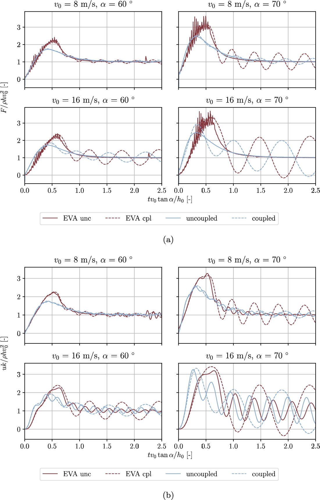
The response of the wall is shown in Fig. 6b and the response becomes increasingly dynamic with increasing angle α or velocity v0. As the impact has a higher velocity or steeper angle, the interaction is increasingly important. This is based on two load characteristics: the load rise time is such that it easier excites the structure and the load magnitude such that it is felt by the structure. What is however strange is that the difference in response of the one way and coupled solutions is not the same for EVA and the reduced order model. One reason for this is that the loads have the same force integral but with different maxima. Hence, the peak and force as function of time are different, and these parameters are of importance for the dynamic response. Another reason is that the run up along the wall is different, meaning that if the structure starts to move, it has a different added mass moving along.

We also see that the response of the structure after the impact does not damp out. Over time mass enters the domain with a velocity, therefore adding energy. We expect that the coupled system response will not die out, so a sensible cut-off time should be taken. A simple proposal is the time when the water column in front of the structure exceeds the structure size, or when the uncoupled wall force stabilizes (within a margin) to the expected steady wall force of Equation (32). Here, we took a dimensionless time of τ=0.5.

For the 8 m/s impact velocity the impact forces almost coincide for coupled and uncoupled, just the load case with a 70° wedge angle shows a deviation for all time. The 8 m/s, 60° impact is just slightly decreased by the moving structure. With the fast 16 m/s impact a much larger difference is observed, clearly showing the vibration of the structure in the load. We can see that the coupled solution can result in a higher load on the structure than the uncoupled solution. There is a simple explanation: the structure moves along with the fluid but at some point has to come back. When it does, the relative velocity of the fluid with respect to the structure is increased, therefore increasing the load. This all happens at a time scale where the dynamics of the structure is important. In other words: whether the load is increased due to FSI is very dependent on the dynamics of the load and structure.

Finally, it should be noted that Table 1 gives the duration of the final vibration period. We can see a big difference between the coupled and uncoupled structures, where the coupled response is almost the same for both solvers. Physically this means the added mass for both solvers is approximately the same. Furthermore, even though the impact maximum is equal, the NHSWE solver does say something about the effect of FSI and it could be a valuable tool to check the system sensitivity with respect to the coupling.

From Table 1 we can also see the height of the last peak for coupled or uncoupled response is the same. It means that we do predict approximately correctly how much energy is absorbed by the structure, and whether the FSI is amplifying the response or diminishing it. The added benefit of the reduced order model is that it is much faster than the high fidelity method in doing so, in the order of a few minutes versus a day of computation time.

3.2.Variation of impact angle and velocity

Fig. 7.

Contour plot of the ratio between coupled and uncoupled force on the wall and displacement of the wall. If the value is larger than unity the force or displacement in the coupled case is higher than for the uncoupled case. Unity is marked with the white contour lines. The black dashed lines are the critical times from equation (30). The initial height is kept constant at h0=0.2 m.

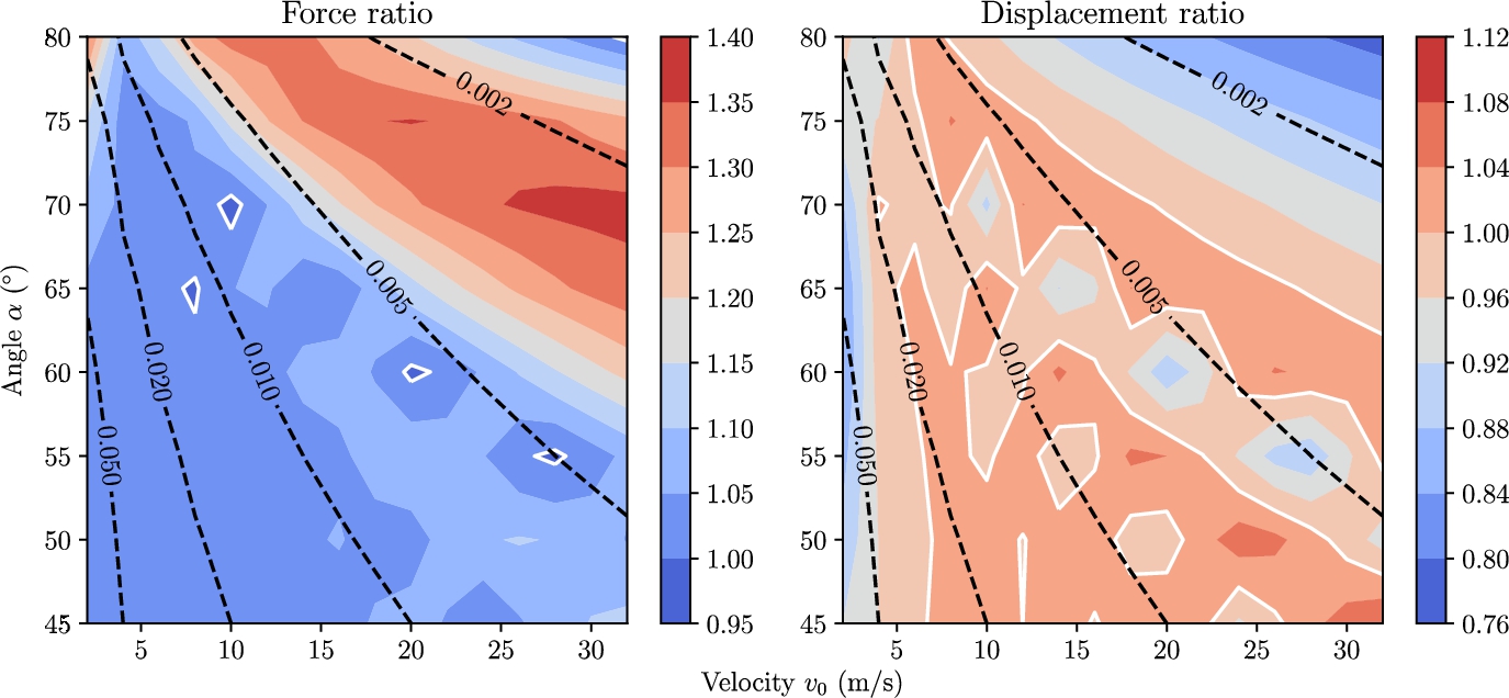
The low fidelity model can be used to check the effect of different angles and impact velocities, as an example of a sensitivity study. Figure 7 shows a study of the difference between coupled and uncoupled impacts for angles between α=45∘…80∘ and v0=2…32 m/s. The other parameters such as fluid density, fluid height and the structural parameters are kept the same as previously. In the graphs a contour plot of the ratio of force or displacement is shown, the coupled result divided by the uncoupled one. Also contours are shown of the critical time tc, as defined in Equation (30), which was earlier defined as a measure when the wedge has fully been absorbed by the wall. Only results related to the peak of the wedge impact are used, not the (numerical) direct impact nor any vibrations after 1.25·tc.

It is clear from the both graphs that the lines of the ratio have similar alignment as the lines of the critical time. Especially the critical time tc=0.005 s is close to the wet natural period, and tc=0.002 s is close to the dry natural periods (see Table 1). This indicates that whether FSI affects the result depends on the critical time of the loading compared to the natural period of the structure. Not a surprising conclusion, but an important one considering how easy it is to calculate the critical time and natural period of the structure.

It is clear from the left plot in Fig. 7 that the maximum force of the coupled calculation is in almost all cases higher than for the uncoupled calculation. As mentioned before, this is attributed to the structure first moving along with the impact, but after some time coming back, that is when the maximum force is reached. According to this figure this mostly happens when the critical time is between the wet and dry natural period.

The right graph is much harder to generalize. It looks like higher angles or velocities might show more that the FSI coupling decreases the response. But, for the other combinations of angle and velocity there is no clear trend, which means that whether the structure is sensitive to FSI depends on the specific impact parameters.

4.Conclusions

Wave impacts onto the wall of an LNG tank are limiting for the design. The interaction between the wave and the wall could increase or decrease the response of the structure. High fidelity models for fluid-structure interaction are typically computationally expensive, which is why we propose a reduced order model for the fluid. The reduced order model is coupled to a reduced order model for the structure, being an order of magnitude faster than the high fidelity model. This reduced order model makes it possible to estimate quickly the effect of hydro-elasticity on the dynamics of the system during a wave impact.

We consider as impact case a cut off wedge, as a model for the wave crest hitting the wall. The reduced order model predicts the same total impulse and added mass as the calculations with EVA, which is an in-house developed CFD code. It shows lower force than EVA, yet it is usable to quantify the sensitivity of the structure response to fluid-structure interaction. This is possible because the total impulse and added mass are almost the same, leading to almost the same final excitation. The difference can be explained by the kinematic assumption used to arrive at the reduced order model and its influence on the maximum force.

An example of a sensitivity study is given, where impact velocity and angle are varied for the same structure. From these results it seems like the force in the coupled calculations is generally higher than for the uncoupled calculations. However, there is not such a clear trend for the displacement of the wall. It was not possible to derive a rule of thumb for the importance of FSI in wave impacts, as it depends strongly on the impact shape and velocity.

For future studies it is recommended to generalize the sensitivity analysis in the sense of dimensionless numbers, for instance the ratio of critical time to vibration period. Maybe in such cases it is easier to draw general conclusions, and look for areas where FSI is never important. The reduced order model can be improved adding functions that describe the velocity field in the impacting wave. Therefore the wave impact forces should be modelled more accurately, as the local flow details are better captured. However, this does come at added complexity and effectively brings the reduced order model closer to EVA. Another improvement would be to stretch the domain with the moving wall, improving accuracy for larger wall deformations.

The aforementioned screening method could calculate the response to a wave impact using the simplified models presented in this paper. Then, the most critical load cases can be further investigated using a high fidelity code. Note that in this paper only a cut-off wedge is used for the impact, but the shape can be much more general.

Funding

This work is part of the research programme ‘SLING’ with project number P14-10 which is (partly) financed by the Netherlands Organisation for Scientific Research (NWO).

Conflict of Interest

M. van der Eijk and P.R. Wellens are Editorial Board Members of this journal, but were not involved in the peer-review process nor had access to any information regarding its peer-review.

Author contributions

R.W. Bos: Conceptualization, Methodology, Formal analysis, Investigation, Visualization, Writing – original draft. M. van der Eijk: Methodology, Formal analysis, Investigation, Visualization, J.H. den Besten: Writing – review and editing, Supervision P.R. Wellens: Writing – review and editing, Supervision

References

[1]	R.A. Bagnold, Interim report on wave-pressure research, Journal of the Institution of Civil Engineers 12: ((1939) ), 202–226. doi:10.1680/ijoti.1939.14539.
[2]	H. Bogaert, An Experimental Investigation of Sloshing Impact Physics in Membrane LNG Tanks on Floating Structures, PhD thesis, Delft University of Technology, 2018.
[3]	H. Bogaert, M.L. Kaminski and L. Brosset, Full and large scale wave impact tests for a better understanding of sloshing – results of the sloshel project, in: Proceedings of the International Conference on Ocean, Offshore and Arctic Engineering, (2011) .
[4]	R.W. Bos, J.H. den Besten and M.L. Kaminski, A reduced order model for structural response of the Mark III LNG cargo containment system, International Shipbuilding Progress 66: ((2020) ), 295–313. doi:10.3233/ISP-190272.
[5]	R.W. Bos and M.L. Kaminski, Comparing 2D and 3D linear response of a simplified LNG membrane cargo containment system, in: Proceedings of the International Offshore and Polar Engineering Conference, (2018) , pp. 780–787.
[6]	V. Bureau, Design sloshing loads for LNG membrane tanks, May 2011. Guidance note NI 564 DT R00 E.
[7]	E. Cumberbatch, The impact of a water wedge on a wall, Fluid Mech. 7: ((1959) ), 353–374. doi:10.1017/S002211206000013X.
[8]	F. Dias and J.-M. Ghidaglia, Slamming: Recent Progress in the Evaluation of Impact Pressures, Annual Review of Fluid Mechanics 50 (2018).
[9]	B.A. Finlayson, The Method of Weighted Residuals and Variational Principles, Mathematics in Science and Engineering., Vol. 87: , Academic Press, (1972) .
[10]	T. Gavory and P.-E. de Sèze, Sloshing in membrane LNG carriers and its consequences from a designer’s perspective, International Journal of Offshore and Polar Engineering 19: (4) ((2009) ), 13–20.
[11]	E. Gervaise, P.-E. De Sèze and S. Maillard, Reliability-based methodology for sloshing assessment of membrane LNG vessels, in: Proceedings of the International Offshore and Polar Engineering Conference, (2009) , pp. 254–263.
[12]	GTT \| Mark III systems. https://www.gtt.fr/en/technologies/markiii-systems, accessed 2021-03-30.
[13]	J.A. Issa, L.O. Garza-Rios, R.P. Taylor, S.P. Lele, A.J. Rinehart, W.H. Bray, O.W. Tredennick, G. Canler and K. Chapot, Structural capacities of LNG membrane containment systems, in: Proceedings of the International Offshore and Polar Engineering Conference, (2009) , pp. 107–114.
[14]	A. Jeschke, G.K. Pedersen, S. Vater and J. Behrens, Depth-averaged non-hydrostatic extension for shallow water equations with quadratic vertical pressure profile: Equivalence to Boussinesq-type equations, International Journal for Numerical Methods in Fluids 84: (10) ((2017) ), 569–583. doi:10.1002/fld.4361.
[15]	M.L. Kaminski and H. Bogaert, Full-scale sloshing impact tests- part I, International Journal of Offshore and Polar Engineering 20: (1) ((2010) ), 24–33.
[16]	M.H. Kim, S.M. Lee, J.M. Lee, B.J. Noh and W.S. Kim, Fatigue strength assessment of mark-iii type lng cargo containment system, Ocean Engineering 37: ((2010) ), 1243–1252. doi:10.1016/j.oceaneng.2010.05.004.
[17]	W. Lafeber, L. Brosset and H. Bogaert, Elementary loading processes (ELP) involved in breaking wave impacts: Findings from the Sloshel project, in: Proceedings of the International Offshore and Polar Engineering Conference, (2012) , pp. 265–276.
[18]	C. Lugni, A. Bardazzi, O.M. Faltinsen and G. Graziani, Hydroelastic slamming response in the evolution of a flip-through event during shallow-liquid sloshing, Physics of Fluids 26 (2014).
[19]	S. Malenica, I. Ten, T. Gazzola, Z. Mravak, J. De-Lauzon, A.A. Korobkin and Y.M. Scolan, Combined semi-analytical and finite element approach for hydro structure interactions during sloshing impacts – “Sloshel project”, in: Proceedings of the International Conference on Offshore Mechanics and Arctic Engineering, (2009) .
[20]	P. Navarro, S. Abrate, J. Aubry, S. Marguet and J.-F. Ferrero, Analytical modeling of indentation of composite sandwich beam, Compos. Struct. 100: ((2013) ), 79–88. doi:10.1016/j.compstruct.2012.12.017.
[21]	B. Pillon, M. Marhem, G. Leclèrce and G. Canler, Numerical approach for structural assessment of LNG containment systems, in: Proceedings of the International Offshore and Polar Engineering Conference, (2009) , pp. 175–182.
[22]	G. Stelling and M. Zijlema, An accurate and efficient finite-difference algorithm for non-hydrostatic free-surface flow with application to wave propagation, International Journal for Numerical Methods in Fluids 43: ((2003) ), 1–23. doi:10.1002/fld.595.
[23]	M. van der Eijk and P.R. Wellens, A compressible two-phase flow model for pressure oscillations in air entrapments following green water impact events on ships, International Shipbuilding Progress (2019), 1–29.
[24]	V.Z. Vlasov and N.N. Leont’ev, Beams, Plates and Shells on Elastic Foundations, Israel Program for Scientific Translations, (1960) .
[25]	H. Wagner, Über Stoß- und Gleitvorgänge an der Oberfläche von Flüssigkeiten, Zeitschrift für Angewandte Mathematik und Mechanik 12 (1932).
[26]	P. Wellens and M. Borsboom, A generating and absorbing boundary condition for dispersive waves in detailed simulations of free-surface flow interaction with marine structures, Computers and Fluids 200 (2020).
[27]	Y. Yamazaki, Z. Kowalik and K.F. Cheung, Depth-integrated, non-hydrostatic model for wave breaking and run-up, Int. J. Numer. Meth. Fluids 61: ((2009) ), 473–497. doi:10.1002/fld.1952.
[28]	Y. Zhang and D. Wan, Mps-fem coupled method for sloshing flows in an elastic tank, Ocean Engineering 152: ((2018) ), 416–427. doi:10.1016/j.oceaneng.2017.12.008.
[29]	R. Zhao and O. Faltinsen, Water entry of two-dimensional bodies, J. Fluid. Mech. 246: ((1993) ), 593–612. doi:10.1017/S002211209300028X.