
An experimental study on added resistance focused on the effects of bow wave breaking and relative wave measurements
Abstract
The added resistance is a resistance component that is not yet satisfactorily predicted, although its accurate estimation is crucial – both from an environmental and economic point of view – from the design stage of a ship until its operation. One of the possible sources of overprediction is the occurrence of bow wave breaking. The first aim of this paper is to study the effect of bow wave breaking on added resistance by combining visual observations with resistance tests. On the other hand, as the bow region of a ship appears to be the most dominant contributor to added resistance, this paper introduces a dynamic waterline detection method involving stereo vision. This experimental method is applied to reach the second aim of this paper, which is to stress the importance of the relative wave elevation in the bow region of the ship. By placing stereo rigs inside the hull of a semi-transparent ship, the waterline at each momnent in time can be tracked using an edge detection algorithm. By performing resistance tests on the Delft Systematic Deadrise Series ship model no. 523, the added resistance is observed to be proportional to the relative wave height squared. The data of the experiment and the information necessary to reproduce the experiment are shared through https://doi.org/10.4121/19525852.
1.Introduction
The increased attention for the environment through the introduction of efficiency indices such as the EEDI and EEOI [11] stimulates increasing the energy efficiency of ships. This leads to a particular interest in added resistance in waves, a resistance component that is currently hard to predict. One of the uncertainties lies within the phenomenon of bow wave breaking, which is expected to have a nonlinear, reducing, impact on added resistance. If current methods overestimate added resistance, the installed engine capacity may also be too high. With a better understanding of bow wave breaking on added resistance, less powerful engines could potentially be installed which in turn would lead to more efficient ship designs. A literature review reveals different studies, [10,19] and [16], who pinpoint the breaking of the bow wave as a possible source for the difference in added resistance without quantifying its effect.
Only Choi et al. [3,4] venture into an attempt to distinguish bow wave breaking effects. Choi and Huijsmans [3] explicitly focus on the nonlinearity of added resistance induced by bow wave breaking and proposed a new transfer function representing the nonlinearity for a Fast Displacement Ship. In a subsequent experimental study, Choi et al. [4] investigated the nonlinear relationship between hull pressure, relative wave elevation, and added resistance for the Fast Displacement Ship and observed a pressure drop caused by the overturning detachment of the bow wave. These results are valid for one type of ship in specific conditions and lack broad applicability. A better understanding of the phenomenon is key to improve the accuracy of added resistance estimates. A parameter that can provide insight into added resistance is the relative wave elevation.
The purpose of this paper is therefore twofold. On the one hand, it aims to relate bow wave breaking to added resistance. On the other, it aims to stress the importance of the relative wave elevation in the bow region of the ship. For that latter objective, this study introduces an experimental method for dynamic waterline detection using stereo vision. In this paper, first, the experimental setup is described, followed by the introduction of the waterline detection methodology. In the section presenting the results, a categorization of bow wave breaking over the different conditions is made and compared with the added resistance results. Subsequently, the relative wave height in the bow region is studied and related to added resistance through the introduction of an alternative added resistance coefficient. The data of the experiment and the information necessary to reproduce the experiment are shared through https://doi.org/10.4121/19525852.
2.Experimental setup
2.1.Facility
Table 1
Main dimensions of towing tank no.1 and its fluid characteristics during the experiments (mean values, together with the range towards the maximum and minimum values measured)
| Parameter | Value |
| Length of the towing tank | 142.00 m |
| Width of the towing tank | 4.22 m |
| Water depth | ( |
| Water temperature | ( |
| Water density | ( |
The experimental work was performed using the facilities of the Ship Hydrodynamic Laboratory of Delft University of Technology. The setup of the experiment is connected to the motor-driven carriage of towing tank no. 1 of the 3ME faculty, a freshwater basin. The towing tank is equipped with an electronic/hydraulic flap-type wave maker, which can produce wavelengths between 0.30 and 6.00 m long and can produce both regular and irregular waves. This makes the facility suited for added resistance tests. The tank dimensions and its fluid characteristics are given in Table 1. The ranges for water depth, temperature and density indicate the variation in measurements during the two weeks of experimental campaign. For instance, temperatures varying between 14.9 and 15.9 degrees were measured.
2.2.Ship model
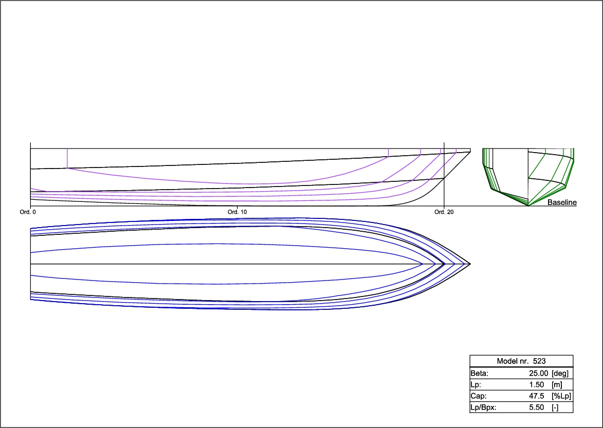
The ship model no. 523 is chosen, a hard chine planing hull from the Delft Systematic Deadrise Series with a deadrise of 25 deg, a twist angle of 10 deg and a negative buttock angle of 1.69 deg [15]. In order to check the setup, the resistance curve of the model is determined up to
Table 2
Main particulars of the DSDS model no. 523
| Particulars | Units | Model scale | |
| Length between perpendiculars | m | 1.500 | |
| Length on waterline | m | 1.517 | |
| Breadth Moulded | B | m | 0.330 |
| Depth moulded | D | m | 0.207 |
| Displacement | ∇ | m3 | 0.025 |
| Mass | m | kg | 25.36 |
| Trim (forward positive) | t | degrees | 0.667 |
| Mean draft | T | m | 0.107 |
| Block coefficient | – | 0.477 | |
| Waterplane area | m2 | 0.390 | |
| Wetted surface | S | m2 | 0.515 |
| Form factor [9] | k | – | 0.648 |
| Vertical center of gravity | VCG | m | 0.159 |
| Longitudinal center of gravity | LCG | m | 0.712 |
| Roll radius of gyration | m | 0.373 | |
| Pitch radius of gyration | m | 0.542 | |
| Yaw radius of gyration | m | 0.617 |
Fig. 1.
Lines plan of the DSDS model no. 523.
2.3.Measurement setup
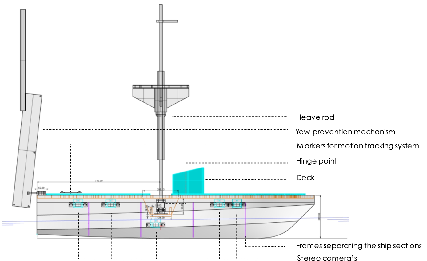
During the tests, the ship model is towed by the tank carriage at constant speed with pitch and heave the only degrees of freedom, as different studies state that surge has a very limited effect on added resistance [2,6,16]. The hinge that permits rotation is located 0.712 m forward of the stern and 0.160 m above the bottom line, in the center of gravity of the ship. Our experimental setup extends the standard resistance test setup with one for optical measurements of the waterline. The setup is shown in Figs 2 and 4.
Fig. 2.
Side view of the DSDS model no. 523 setup including placement of the mechanisms ensuring correct degrees of freedom, the Certus plate and the stereo rigs.
The test campaign involves the following measured quantities:
Resistance measurements, using a load cell with a capacity of 100 N. This capacity is based on the forces induced by the acceleration, deceleration and the still water resistance predicted using the method developed by Holtrop and Mennen [9] and backed by the resistance measurements done during de DSDS campaign. The advice of the ITTC to use twice the still water resistance for the capacity for the load cell is followed [13]. Only the longitudinal component of the forces is measured.
Pitch and heave measurements, using an Optotrak Certus motion tracking system. Its position sensor, fixed to the carriage, detects the markers placed on a plate positioned on the top deck of the ship model.
Relative wave height measurements, using a stereo rig setup constituted of five Arducam 1MP*2 Stereo Cameras with Dual OV9281 Monochrome Global Shutter Camera Module. These are distributed on the port side of each of the five sections of the model such that their fields of view cover the semi-transparent starboard side of the ship model, as visible in Fig. 3. These cameras are controlled by five Raspberry Pi 4B+, also attached to the deck of the ship model. This setup thus includes single-board computers, stereo cameras, power supplies and cables for communication and power.
Wave measurements, using acoustic wave probes. One of the wave probes is located at the same longitudinal position as the rotation point of the ship, 1.5 m on its port side. The other one is located 1.1 m ahead of the rotation point and 0.55 m to the starboard side.
Carriage position and speed, using a laser and a tachometer.
Temperature, on a daily basis as suggested by the ITTC [12] using a thermometer.
Water level, verified on a daily basis.
All values are measured at a rate of 1000 Hz and downsampled to a rate of 100 Hz, except for the photos taken by the stereo cameras, which are taken at a rate of 25 Hz.
Fig. 3.
Top view of the two foremost sections. The deck is removed such that the stereo rig setup is visible. The stereo cameras are oriented towards the semi-transparent half of the ship model.
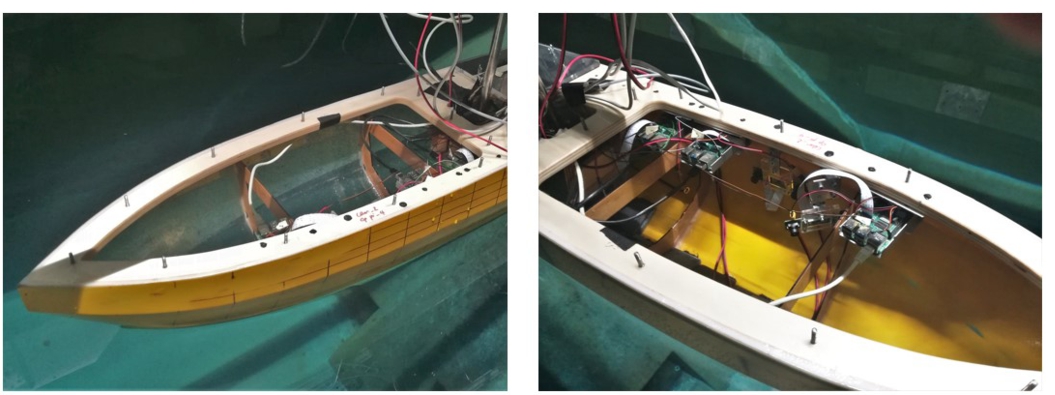
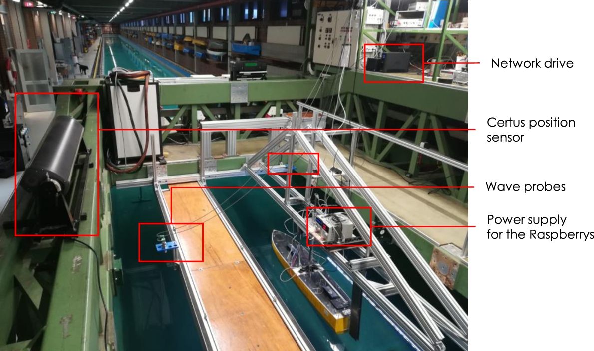
Fig. 4.
Picture of the carriage supporting the setup.
2.4.Experimental conditions
Experiments are performed both in calm water and in regular waves. Each condition is repeated at least three times, spread over different testing days in order to check repeatability. In between runs, a waiting time of 15 to 30 minutes is maintained in order to minimize the effect of remaining waves in the towing tank.
For calm water, a range of speeds between a Froude number of 0.15 to 0.9 is selected. In waves, a speed range corresponding to a Froude number of
Following the Netherlands Regulatory Framework (NeRF, [5]), head sea conditions are appropriate to represent the environmental conditions for the computation of the weather factor which is needed for the computation of energy indices. Therefore, a 180 degree heading is chosen for the experiments in waves.
Tests are done for short, intermediate and long wavelengths, i.e. for
Table 3
Regular wave conditions
| Targeted | Realised | ||
| Wave length [m] | Wave steepness | Wave length [m] | Wave steepness |
| 0.75 | 0.017 | 0.75 | 0.019 |
| 0.75 | 0.020 | 0.75 | 0.023 |
| 0.75 | 0.025 | 0.75 | 0.031 |
| 1.65 | 0.017 | 1.65 | 0.015 |
| 1.65 | 0.020 | 1.65 | 0.019 |
| 1.65 | 0.025 | 1.65 | 0.025 |
| 3.00 | 0.017 | 3.00 | 0.016 |
| 3.00 | 0.020 | 3.00 | 0.020 |
| 3.00 | 0.025 | 3.00 | 0.025 |
Before starting the measurements, all used sensors are checked and calibrated. The main estimated error margins are summarized in Table 4. The reported errors are the maximum deviations with respect to the calibration. The motion tracking sensor is calibrated in different steps by comparing the measured motion when driving the carriage forward and when moving the motion sensor plate sideways manually. The error was measured to be within 0.01 deg for pitch. For heave, the Certus system is accurate to 0.001 m. The wave probes are calibrated in two steps, by measuring the distance to the free surface at four positions on the carriage in steps of 0.04 m resulting in an error of 0.001 m. The load cell is calibrated twice in twenty steps. The accuracy of the load cell is measured to be 0.3 N; this is 0.3% of the range of the load cell.
After calibrating the cameras and reconstructing the ship sections, the distance between reference points drawn on the hull shows an error in vertical direction and in horizontal direction that is smaller than between drawing and model. For the waterline detection, see Section 3, the adopted approach leads to an uncertainty of 3 pixels in vertical direction, corresponding to 2.18 mm in the most forward section and 1.18 mm in the second section.
Table 4
Margin of error for the main measuring devices
| Measurand | Measurement error |
| Certus motion tracking system | 0.001 m in heave direction |
| 0.01 deg in pitch direction | |
| Load cell | 0.3 N |
| Wave probes | 0.001 m |
| Waterline detection | 0.002 m |
3.Waterline detection methodology
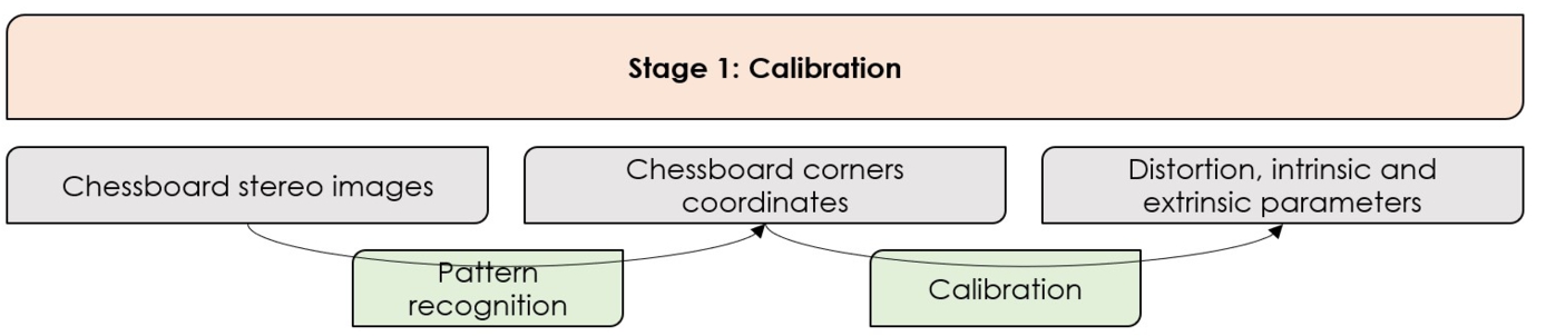
The methodology to detect the waterline through stereo vision can be divided into three phases: 1) Camera calibration, 2) 3D hull reconstruction and 3) Waterline detection, shown in Figs. 5, 6 and 7, respectively. Each of these phases is subdivided into several steps.
First of all, calibrating the cameras is crucial for 3D reconstructions since it allows relating the camera’s units (pixels) to physical units in the 3D world (meters). The output of this step includes the distortion, intrinsic and extrinsic parameters of the camera [1]. To this end, a well-defined pattern should be chosen to represent the calibration target, e.g. a 9x6 chessboard with squares of 1 cm2. As shown in Fig. 5, the calibration phase is subdivided into two steps, being firstly the pattern recognition from a series of pictures taken of the calibration target and secondly the derivation of all camera characteristics from these recognized patterns.
Fig. 5.
Waterline detection: diagram showing the steps of Stage 1. It is divided into three layers, being from top to bottom 1) Stage name, 2) input/output, 3) action.
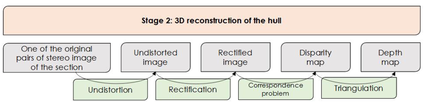
Secondly, the calibration stage is followed by the 3D reconstruction of the ship hull. This is done in four steps, as shown in Fig. 6. The undistortion and rectification steps are performed using the output of the first stage, the camera’s characteristics. After these two steps, a coplanar, row-aligned image is obtained. During the third step, the correspondence between both images, i.e. the image made by the left and right lens of the dual camera, is assessed. Matching features in both images is called the stereo correspondence problem and results in a disparity map. In the current study, the correspondence problem is solved with the Semi Global Block Matching algorithm [7]. During this project, the homogeneous color the ship hull led to challenges in creating the disparity map. Therefore, a random 3D pattern was drawn on the hull, which can be seen in Fig. 8 and 9. This has shown to be an effective way to improve the disparity map. In the fourth step of this stage, triangulation is applied to reproject the feature in 3D coordinates, cf. [1] for an overview of the process. It transforms the disparity map to a depth map, as the disparity is inversely proportional to the distance between the stereo camera and the feature in question.
Fig. 6.
Waterline detection: diagram showing the steps of Stage 2. It is divided into three layers, being from top to bottom 1) Stage name, 2) input/output, 3) action.
The third and last stage, the waterline detection, only needs the images captured by one of the lenses during an experimental run. In this study, the left lens of the stereo cameras is chosen. This left image is first rectified and undistorted with the calibration parameters derived in Stage 1. Then, during the first filtering step, the brightness and contrast of the image are increased by a factor of two and the image is blurred with a Gaussian filter in order to remove speckles and noise. Next, a Canny edge algorithm is applied which computes the intensity gradient using a Sobel kernel as approximation method [17]. This step relies on the fact that light is directed through the hull above water level and on the lack of luminosity below water level such that the pattern on the hull there is not recognized by the Canny edge algorithm. The resulting image is shown in Fig. 8. The obtained edges are then dilated and eroded by a squared kernel of 3 pixels in order to fill small holes and filter out small detected objects. The lowest pixel in each column of pixels is selected to be the waterline. Then, a second filtering step is performed in which the waterline is filtered. The outliers are removed based on the median and replaced when necessary by the neighbouring value. This filter identifies an element as being an outlier when it is further from the mean than 3 scaled median absolute deviations (MAD) away from the median. To smooth the dataset, a second-order Savitsky Golay filter is applied. Due to lack of contrast, the edge detection is less reliable in some regions, see the left and right end of the detected line in Fig. 9. Therefore, these regions are left out. The obtained waterline is subsequently mapped from pixel to world coordinates using the output depth map from Stage 2. The 3D point cloud is defined with respect to the camera’s position and orientation. In order to determine the homogeneous affine transformation required to obtain the point cloud with respect to the ship’s coordinate system, three points are drawn on the hull of each section, within the field of view of the camera lenses. The coordinates of the three points of each section with respect to the stern of the ship and the coordinates of those three points with respect to the cameras are known. Using the coordinates, the transformation matrix, which combines both the translation vector and the rotation matrix, can be completed. An example of the resulting waterline is shown in Fig. 10.
Fig. 7.
Waterline detection: diagram showing the steps of Stage 3. It is divided into three layers, being from top to bottom 1) Stage name, 2) input/output, 3) action.
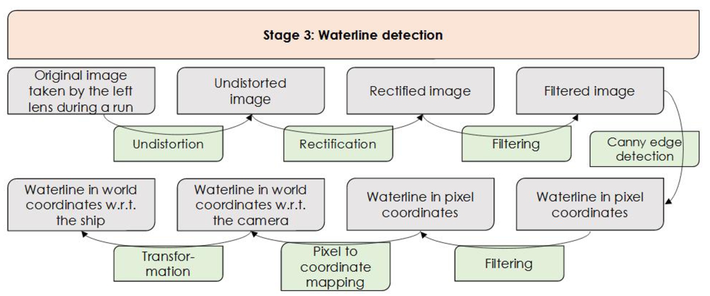
Fig. 8.
Waterline detection: result after applying the Canny edge detection. The random pattern drawn on the hull to improve the disparity map is only detected above water level. The waterline itself is clearly distinguished. The edges detected on the side of the frame and at the bottom of the image are removed using a mask.
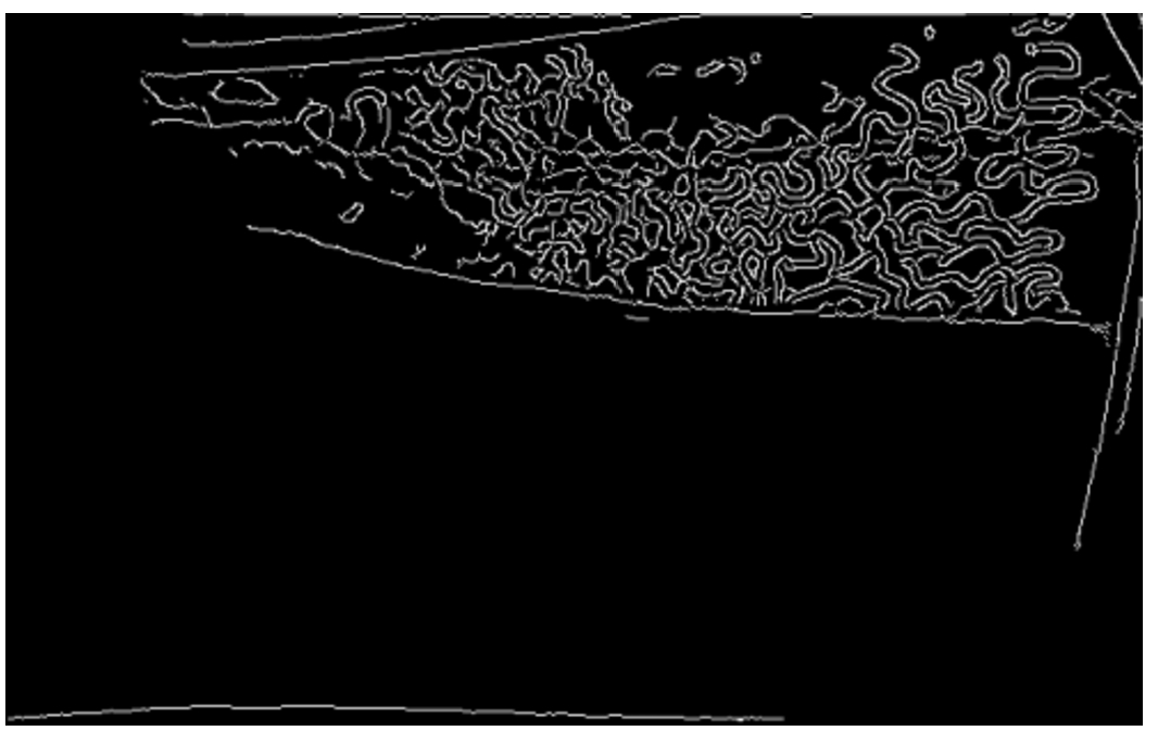
Fig. 9.
Waterline detection: from the edges detected in Fig. 8, the lowest pixels are selected using the assumption that the drawn pattern is not recognized below water level. In this figure, the detected waterline is drawn in white on top of the undistorted rectified left image of the stereo pair.
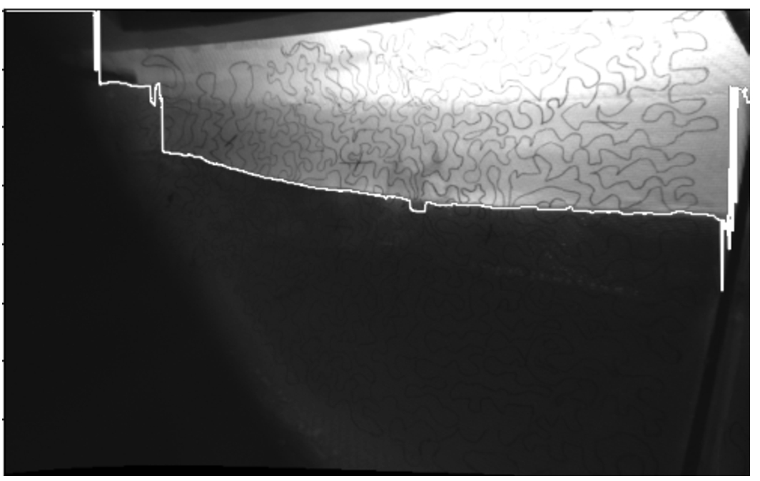
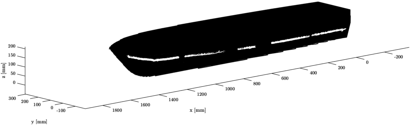
Fig. 10.
Waterline as detected in Fig. 9 is mapped to the 3D point cloud and transformed to be plotted onto the 3D model. The waterline follows the hull well, apart from a few points that are misplaced because of irregularities in the disparity map and the resulting point cloud. The waterline is interrupted where the stiffeners of the hull are in the camera’s field of view.
4.Results and discussion
Calm water results. The calm water runs have three main goals. Firstly, the intent is to determine the resistance curve necessary to compute the added resistance later on. Secondly, the resistance curve can be compared to the one in the DSDS database. And, thirdly, the runs are also intended to identify the regime in which bow waves start breaking in order to select the ship speed range for the regular wave runs.
Fig. 11.
Resistance curve over a range of Froude numbers between
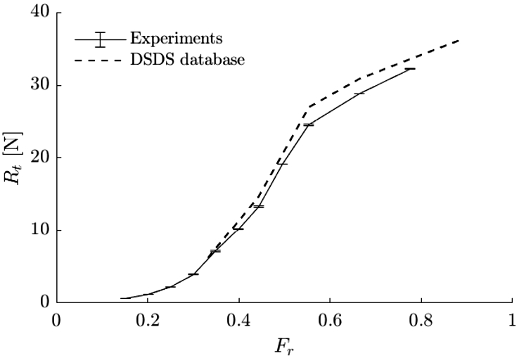
Figure 11 shows the resistance curve of the DSDS model no. 523 for its current loading condition. The values are also included in Appendix B. The difference with previous experiments [15] can be explained by the spray strips that have been removed for the current application and the slightly different draft and location of the center of gravity. This discrepancy increases with speed but stays within 9.60% difference at much higher
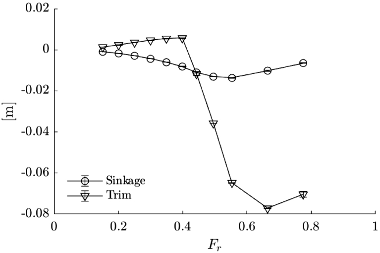
Fig. 12.
Trim and sinkage as measured during the calm water runs.
A broad range of speeds is tested in calm water, from which four are selected to be used during the head sea conditions. The main criterion for this selection is the breaking of the bow wave since the goal is to cross the forward speed at which the bow wave starts breaking. Figures 13, 14, 15 and 16 show the bow wave for the four selected speeds. The free surface disturbances become more apparent with increasing speed until a plunging breaker is distinguishable for
Fig. 13.
Front view of the ship model advancing through the towing tank at
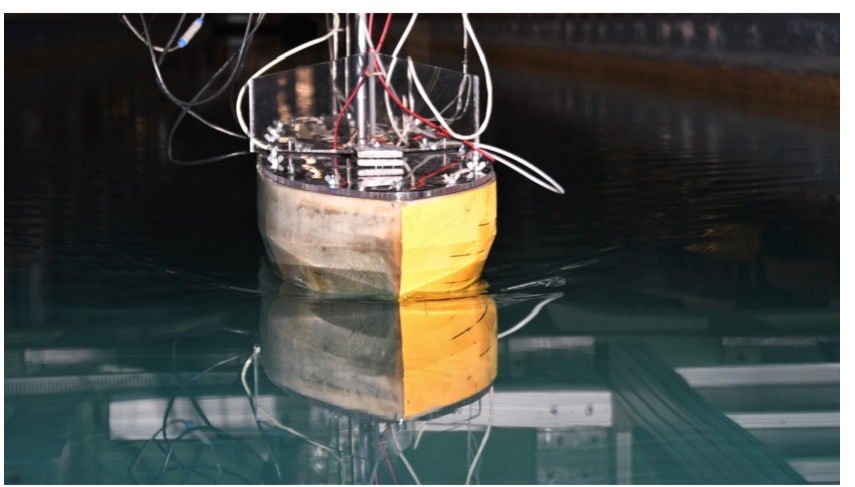
Fig. 14.
Front view of the ship model advancing through the towing tank at
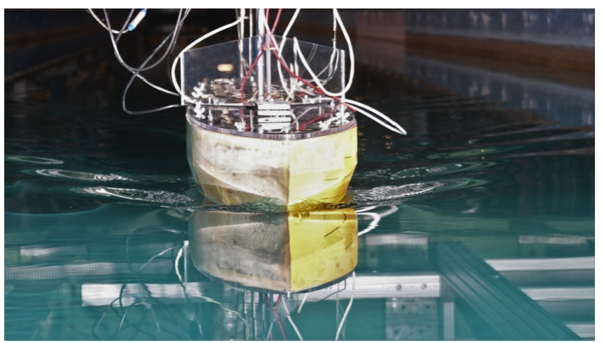
Fig. 15.
Front view of the ship model advancing through the towing tank at
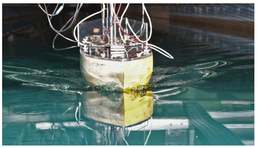
Fig. 16.
Front view of the ship model advancing through the towing tank at
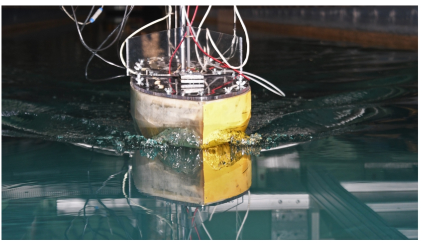
Table 5
Categorization of bow wave breaking in short waves, i.e.
 |  |  | ||
| × | ||||
| × | ||||
| × | ||||
| × | ||||
| × | ||||
| × | ||||
| × | ||||
| × | ||||
| × | ||||
| × | ||||
| × | ||||
| × |
Table 6
Categorization of bow wave breaking in intermediate waves, i.e.
 |  |  | ||
| × | ||||
| × | ||||
| × | ||||
| × | ||||
| × | ||||
| × | ||||
| × | ||||
| × | ||||
| × | ||||
| × | ||||
| × | ||||
| × |
Categorization of the bow wave breaking in regular waves. During the calm water tests no non-stationary effects were encountered that could be confused with propagating free surface waves. When the ship model is exposed to incoming waves, the bow wave shows a different behaviour compared to calm water. Tables 5, 6 and 7 give an overview of the visual observations on the bow wave breaking for short, intermediate and long wave lengths, respectively. Three categories are distinguished: plunging breakers, spilling breakers and non-breaking conditions. Plunging is defined by a clear overturning motion of the wave crest.
Exposing the ship model to regular incoming waves with increasing steepness is expected to lead to a gradual transition from non-breaking to breaking bow wave conditions for the two lowest velocities. For
Table 7
Categorization of bow wave breaking in long waves, i.e.
 |  |  | ||
| × | ||||
| × | ||||
| × | ||||
| × | ||||
| × | ||||
| × | ||||
| × | ||||
| × | ||||
| × | ||||
| × | ||||
| × | ||||
| × |
Effect of breaking bow waves on added resistance. In Fig. 17, 18 and 19, the added resistance coefficient is plotted over measured steepness for different wavelengths and ship forward speeds. The added resistance coefficient is found from
The proportionality between the added resistance and the incoming wave amplitude squared as derived from linear potential flow theory is shown not to hold when increasing the incoming wave steepness. This means that there is more at play with the interaction between incoming waves and the calm water wave system. The observed trends do not correlate with the transitions between breaking categories that have been visually determined in the preceding section. The hypothesis that the onset of bow wave breaking would affect the added resistance is thus not confirmed by these experiments. It thus also disproves the hypothesis formulated by Choi et al. [4] in which the occurrence of a spilling breaker would increase added resistance while the occurrence of a plunging breaker would decrease added resistance.
It is emphasized that the wave steepness is varied between
The ship motions are shown in Appendix A and evolve linearly with increasing incoming wave height. The incoming wave steepness thus does not affect the ship motions. The largest standard deviation over steepness is observed for short waves, which can be attributed to the variations found in the incoming wave height.
So, the discrepancy between a linear interpretation and the measurements cannot be explained by nonlinearities of the incoming waves, nor of the ship motions. Another factor is thus causing nonlinearities in added resistance when incoming wave steepness is increased, which is why the relative free surface elevation was studied.
Studying the relative free surface elevation. The waterline detection methodology presented in this study is used to measure the relative free surface elevation (RFSE) over the bow region, which extends over 34% of the ship length
Fig. 17.
Added resistance coefficient plotted over measured steepness for different forward velocities, short wave conditions
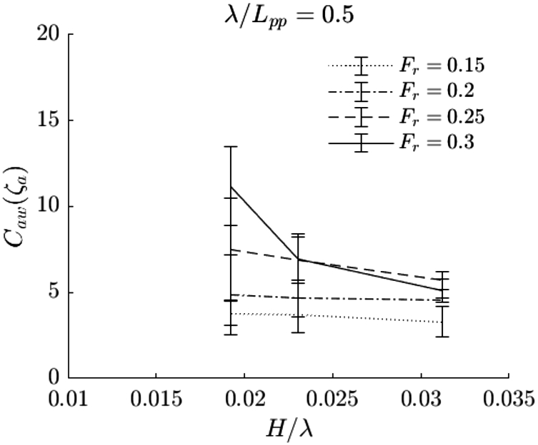
Fig. 18.
Added resistance coefficient plotted over measured steepness for different forward velocities, intermediate wave conditions
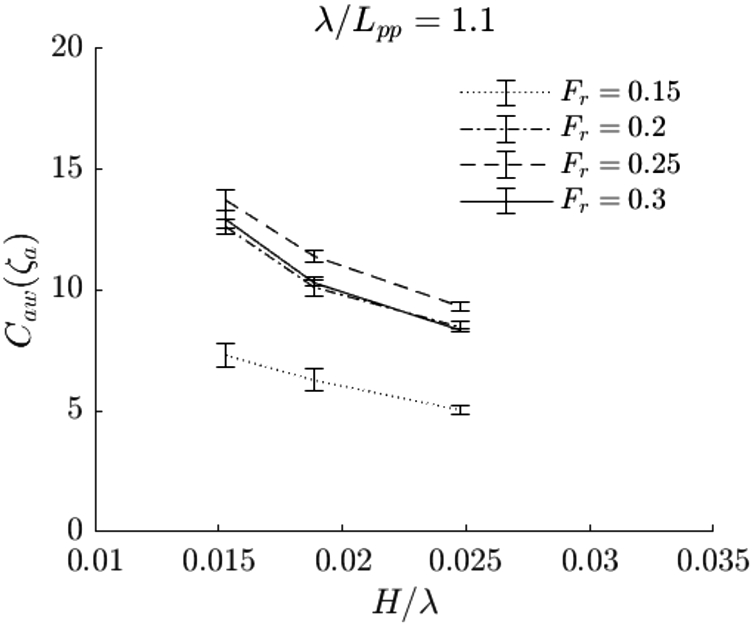
Fig. 19.
Added resistance coefficient plotted over measured steepness for different forward velocities, long wave conditions
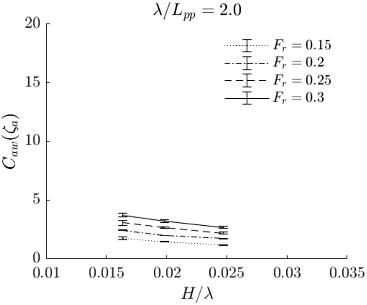
Fig. 20.
Schematic of the relative wave height and relative free surface elevation (RFSE), defined as the maximum variation over time at one location along the ship hull.
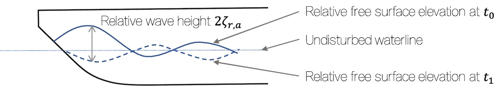
The maximum RFSE remains constant for all bow wave types except plunging breaking bow waves. The maximum RFSE decreases once the bow wave forms a plunging breaking bow wave. This is true for all wave conditions, except for intermediate waves with
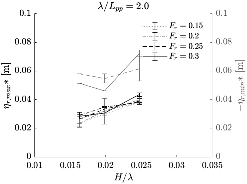
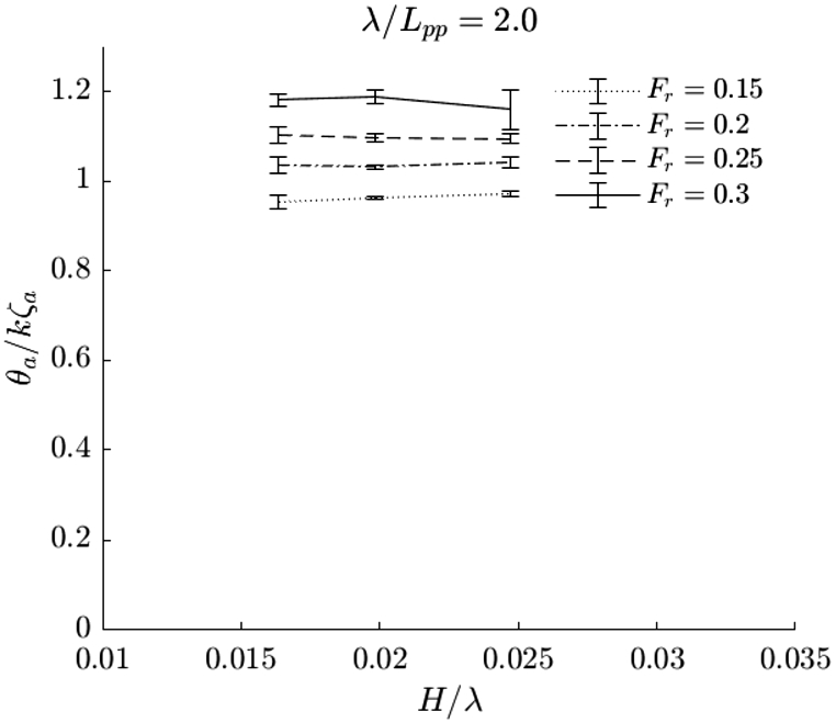
The RFSE is also analysed with respect to the disturbed calm waterline, i.e. the waterline observed when advancing at a constant speed in calm water. The amplitudes of the RFSE are shown in Figs 21, 22 and 23, and are also listed in tables in Appendix C. In the figures, the maxima of the RFSE, which are the amplitudes of the crests, are indicated with black lines; the minima are indicated in grey lines. By observing the RFSE with respect to the calm waterline we can investigate the linearity of the variation of the RFSE near the bow caused by the incoming waves. The variation of the RFSE is linear when crest and trough have equal values, when the values do not change with forward velocity of the ship, and when the values are linear with increasing incoming wave steepness. Only for the longer wave conditions at a Froude number of
Fig. 21.
Maximum (black lines) and minimum (grey lines) relative free surface elevation
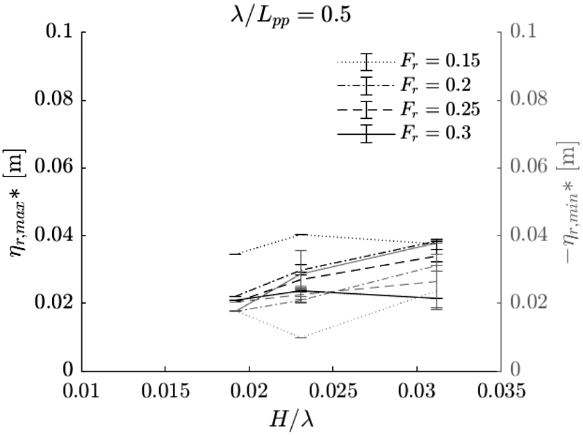
Fig. 22.
Maximum (black) and minimum (grey) relative free surface elevation
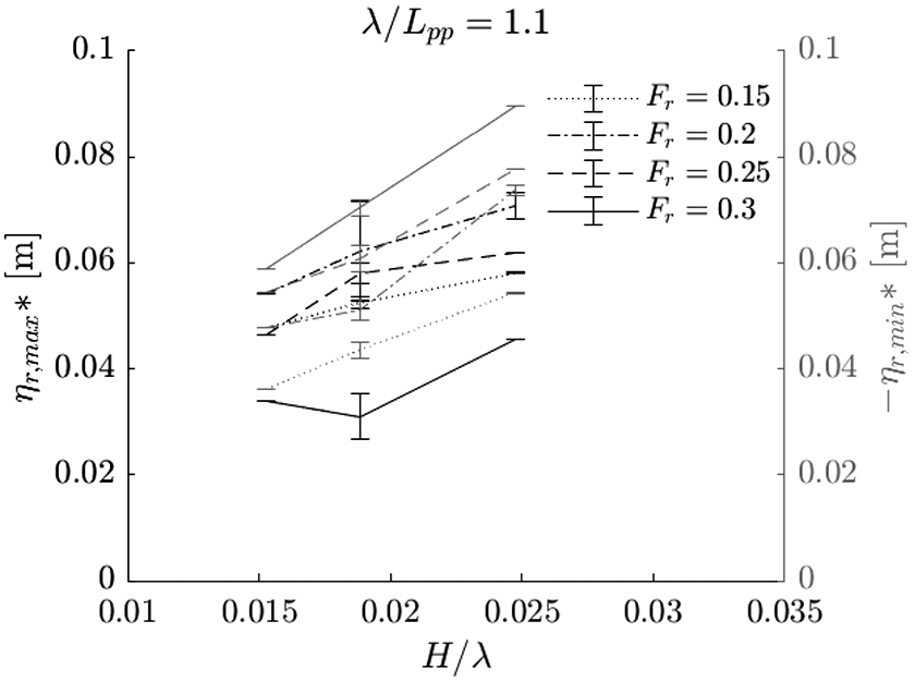
Fig. 23.
Maximum (black) and minimum (grey) relative free surface elevation
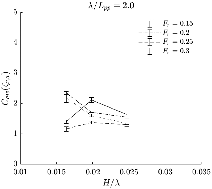
An alternative added resistance coefficient. To relate the relative free surface measurements to the added resistance values, an alternative added resistance coefficient is proposed
This equation is equivalent to the common added resistance coefficient, but scaled by the relative wave height
Fig. 24.
Alternative added resistance coefficient based on the relative wave height plotted over steepness for
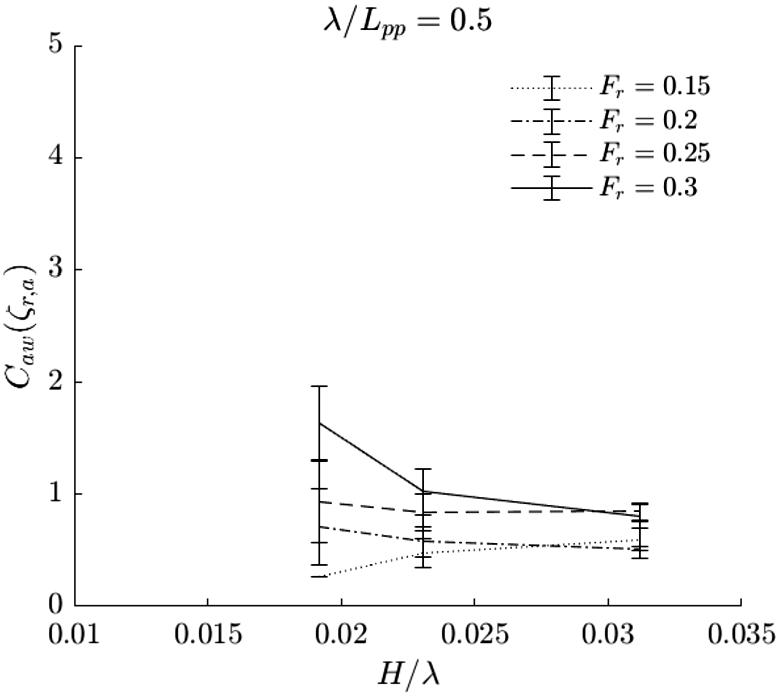
Fig. 25.
Alternative added resistance coefficient based on the relative wave height plotted over steepness for the intermediate wave conditions
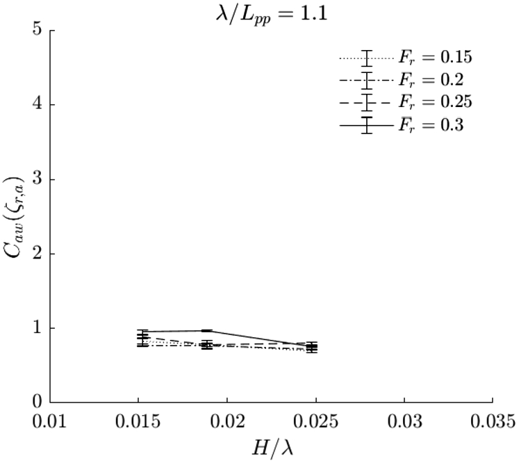
The relative wave amplitude seems to be an appropriate measure to estimate the added resistance over incoming wave steepness and speed, because it greatly reduces the range of values of the alternative added resistance coefficient. The alternative added resistance coefficient
We suspect that the range of values of the alternative added resistance coefficient for the shorter wave conditions in Fig. 24 is somewhat larger because of the accuracy of the wave board’s control system for small period waves with small amplitudes. For the longer wave conditions in Fig. 26, we think that the lack of sensitivity of the force measurement increases the range of values of the coefficient. It is recommended to perform experiments at a larger scale, so that the shorter wave periods are somewhat longer and the forces for the longer wave conditions are somewhat larger.
Fig. 26.
Alternative added resistance coefficient based on the relative wave height plotted over steepness for the longer wave conditions
5.Conclusion
In this paper, added resistance is studied by performing experiments on the DSDS ship model no. 523. During these experiments, the transition between non-breaking and breaking bow wave conditions is crossed for both short and long waves. The results also suggest that linear theory may not be sufficient for the prediction of added resistance, as the commonly used added resistance coefficient was found to decrease with wave steepness. Especially for the tested intermediate wavelength conditions (i.e.
This paper also introduces a novel waterline detection method based on stereo vision which relies on the semi-transparency of the ship hull. In this study, the detection method is applied to measure the relative wave elevation in the bow region. One of the main outcomes of this analysis is the observation of a nonlinear interaction between the incoming waves and the bow wave, resulting in a nonlinear wave pattern along the bow region of the ship hull. In other words, the relative wave height in the bow region is nonlinear.
This study introduces a new added resistance coefficient that scales the added resistance with the relative wave height instead of the incoming wave amplitude. The new added resistance coefficient has much smaller range of values for all tested wave conditions compared to the old coefficient. The new added resistance coefficient has a value close to 1, is constant over wave steepness and independent of the ships forward velocity, especially for intermediate wave conditions (
Appendices
Appendix A.
Appendix A.Ship motions
In this appendix, the results from the ship motion measurements are attached. The appendix also includes results of the resistance measurements and relative wave elevation values. Figure 27, 28 and 29, the dimensionless heave amplitude is plotted. In Fig. 30, 31 and 32, the dimensionless pitch amplitude is plotted over different wave and speed conditions. In these figures, heave is scaled by the incoming wave amplitude and pitch is scaled by the product of the incoming wave amplitude and the incoming wave number.
Fig. 27.
Scaled heave amplitude in short waves, i.e.
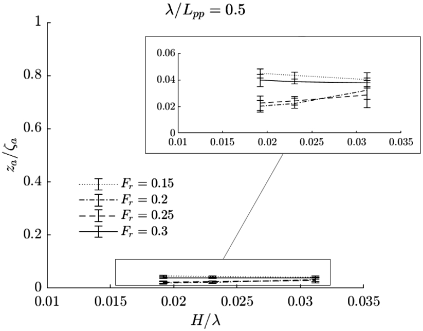
Fig. 28.
Scaled heave amplitude in intermediate waves, i.e.
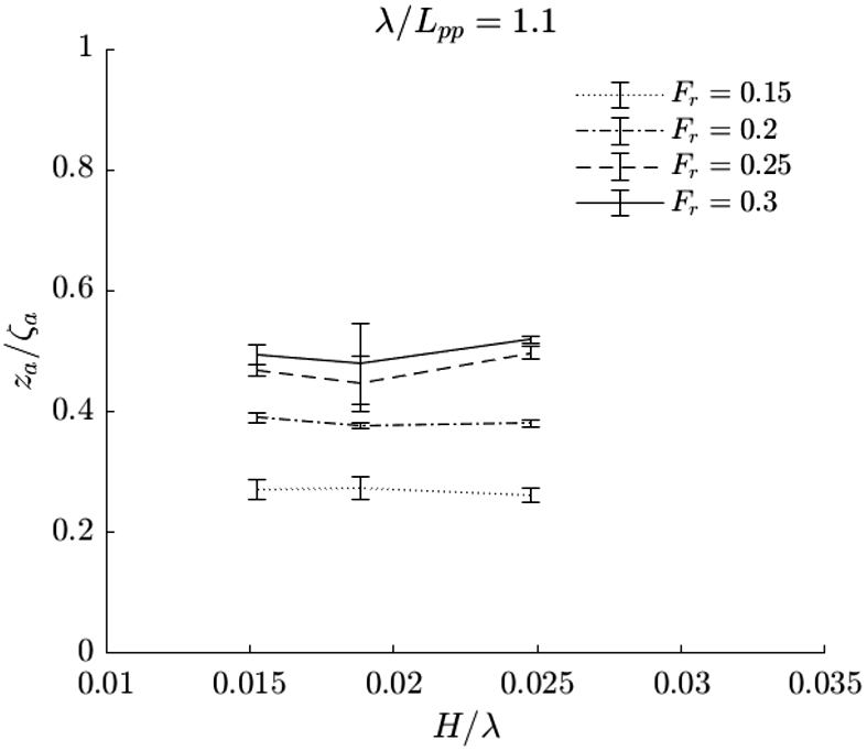
Fig. 29.
Scaled heave amplitude in long waves, i.e.
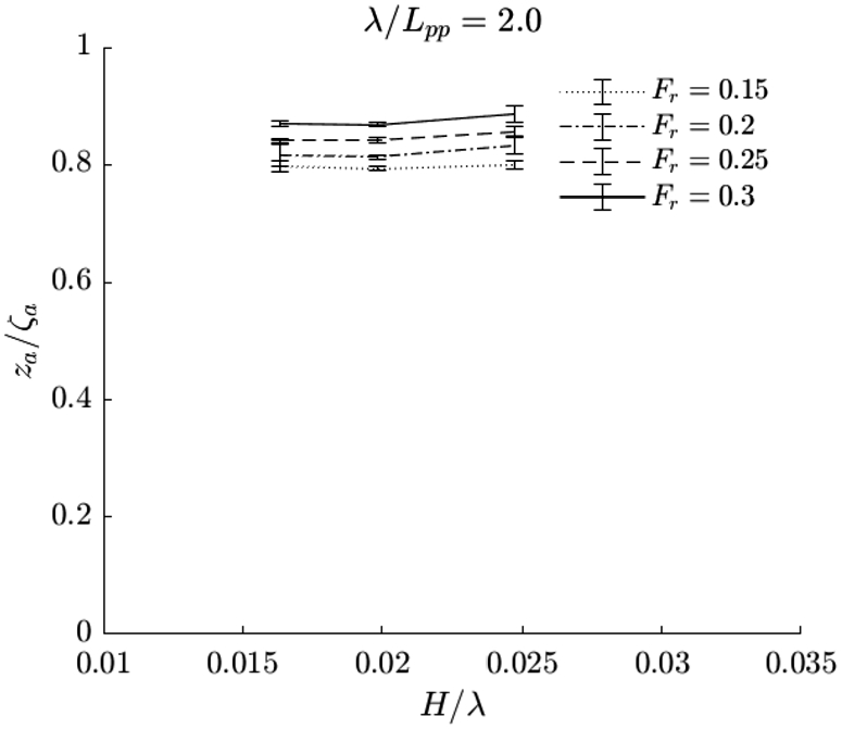
Fig. 30.
Scaled pitch amplitude in short waves, i.e.
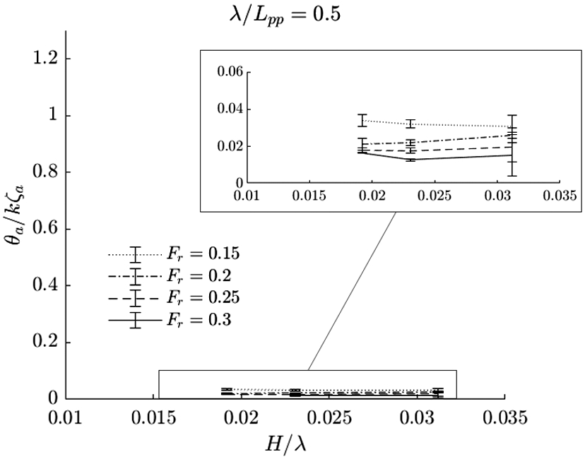
Fig. 31.
Scaled pitch amplitude in intermediate waves, i.e.
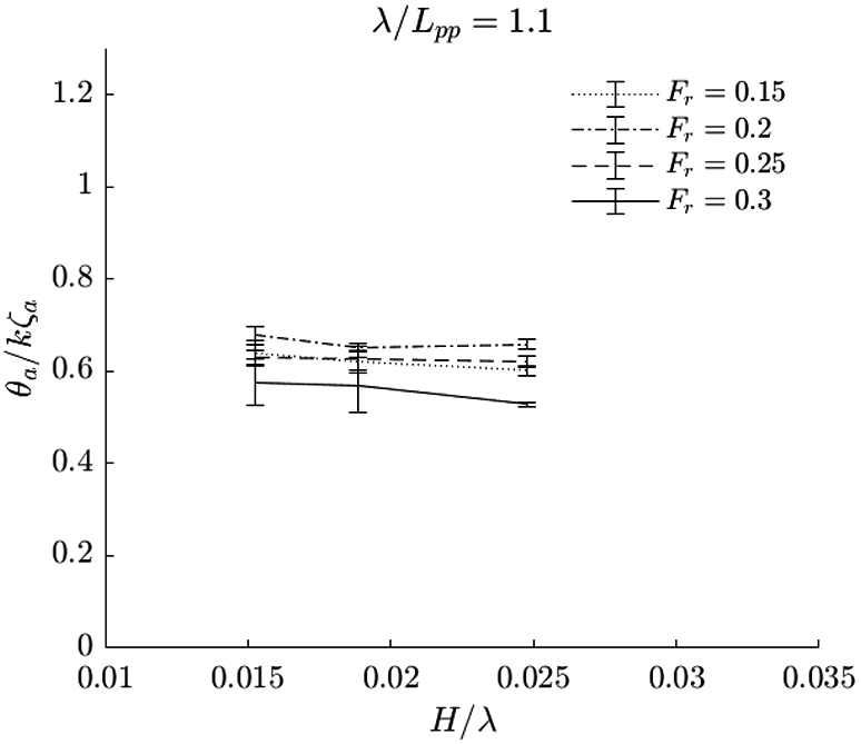
Fig. 32.
Scaled pitch amplitude in long waves, i.e.
Appendix B.
Appendix B.Resistance values
In this appendix, the results for the resistance measurements in calm water are given in Table 8. The resistance in waves is given in Table 9, 10 and 11.
Appendix C.
Appendix C.Relative wave elevation
This appendix presents the maximum and minimum relative wave elevation with respect to the calm waterline. The maximum relative wave elevation, shown in Table 12, 14 and 16, is defined as the distance between the highest elevation along the ship hull reached in waves and the highest elevation along the ship hull in calm water at the same speed. The minimum relative wave elevation, given in Table 13, 15 and 17, is defined as the distance between the lowest elevation along the ship hull reached in waves and the highest elevation along the ship hull in calm water at the same speed.
Table 8
Calm water resistance. The mean value, standard deviation and number of runs are given
| Mean resistance [N] | Standard deviation | Number of runs | |
| 0.58 | 0.635 | 0.02 | 5 |
| 0.77 | 1.165 | 0.019 | 4 |
| 0.96 | 2.177 | 0.003 | 3 |
| 1.15 | 3.927 | 0.047 | 5 |
| 1.34 | 7.143 | 0.091 | 3 |
| 1.53 | 10.22 | 0.074 | 3 |
| 1.699 | 13.324 | 0.075 | 2 |
| 1.77 | 14.257 | 0.157 | 3 |
| 1.9 | 19.164 | 0 | 1 |
| 2.123 | 24.515 | 0.103 | 2 |
| 2.548 | 28.812 | 0.02 | 2 |
| 2.973 | 32.235 | 0.046 | 2 |
Table 9
Resistance in N measured in waves for short wavelength conditions, i.e.
| 0.775 ± 0.027 | 1.344 ± 0.086 | 2.454 ± 0.109 | 4.339 ± 0.085 | |
| 0.831 ± 0.052 | 1.413 ± 0.056 | 2.544 ± 0.072 | 4.297 ± 0.076 | |
| 0.956 ± 0.088 | 1.608 ± 0.014 | 2.732 ± 0.05 | 4.425 ± 0.064 |
Table 10
Resistance in N measured in waves for intermediate wavelength conditions, i.e.
| 1.459 ± 0.057 | 2.592 ± 0.033 | 3.725 ± 0.048 | 5.388 ± 0.042 | |
| 1.717 ± 0.077 | 2.911 ± 0.067 | 4.138 ± 0.046 | 5.699 ± 0.025 | |
| 2.138 ± 0.051 | 3.691 ± 0.062 | 4.953 ± 0.057 | 6.41 ± 0.026 |
Table 11
Resistance in N measured in waves for long wavelength conditions, i.e.
| 1.381 ± 0.052 | 2.207 ± 0.021 | 3.484 ± 0.082 | 5.514 ± 0.064 | |
| 1.554 ± 0.024 | 2.431 ± 0.004 | 3.854 ± 0.057 | 5.94 ± 0.079 | |
| 1.778 ± 0.025 | 2.848 ± 0.035 | 4.308 ± 0.094 | 6.561 ± 0.075 |
Table 12
Maximum relative wave elevation with respect to the calm waterline in cm for short wavelength conditions, i.e.
| 3.44 | 2.22 | 2.03 | 2.09 | |
| 4.03 | 2.99 | 2.7 | 2.36 | |
| 3.74 | 3.84 | 3.41 | 2.14 |
Table 13
Minimum relative wave elevation with respect to the calm waterline in cm for short wavelength conditions, i.e.
| −1.78 | 1.77 | −2.04 | −1.77 | |
| −0.98 | −2.08 | −2.27 | −2.87 | |
| −2.38 | −3.12 | −2.66 | −3.78 |
Table 14
Maximum relative wave elevation with respect to the calm waterline in cm for intermediate wavelength conditions, i.e.
| 4.79 | 5.43 | 4.64 | 3.41 | |
| 5.25 | 6.21 | 5.81 | 3.1 | |
| 5.81 | 7.07 | 6.19 | 4.57 |
Table 15
Minimum relative wave elevation with respect to the calm waterline in cm for intermediate wavelength conditions, i.e.
Table 16
Maximum relative wave elevation with respect to the calm waterline in cm for long wavelength conditions, i.e.
| 2.63 | 2.9 | 2.65 | 2.84 | |
| 3.21 | 3.47 | 3.33 | 3.05 | |
| 3.82 | 3.8 | 3.89 | 4.36 |
Table 17
Minimum relative wave elevation with respect to the calm waterline in cm for long wavelength conditions, i.e.
Acknowledgement
The authors would like to thank J. Rodrigues Monteiro, J. den Ouden, P. Poot, F. Sterk and P. Chabot for their help to prepare and conduct experimental work at the towing tank belonging to the 3ME faculty of the Delft University of Technology.
Conflict of Interest Statement
Peter Wellens is Editor-in-Chief of this journal, but was not involved in the peer-review process nor had access to any information regarding its peer-review.
CREDIT Author Contribution Statement
Author 1: methodology, experiments, formal analysis, writing – original draft, visualization
Author 2: conceptualization, methodology, formal analysis, writing – review & editing
References
[1] | G. Bradski and A. Kaehler, Learning OpenCV, O’Reilly Media, (2008) . |
[2] | S. Chen, T. Hino, N. Ma and X. Gu, RANS investigation of influence of wave steepness on ship motions and added resistance in regular waves, Journal of Marine Science and Technology (Japan) 23: (4) ((2018) ), 991–1003. doi:10.1007/s00773-018-0527-5. |
[3] | B. Choi and R.H.M. Huijsmans, An analysis method to evaluate the added resistance in short waves considering bow wave breaking, in: The 12th International Conference on Hydrodynamics, 18–23 September 2016, Egmond aan Zee, The Netherlands, (2016) . |
[4] | B. Choi, P.R. Wellens and R.H.M. Huijsmans, Experimental assessment of effects of bow-wave breaking on added resistance for the fast ship, International Shipbuilding Progress 66: ((2019) ), 111–143. doi:10.3233/ISP-180242. |
[5] | Dutch Ministry of Infrastructure and Water Management, MEPC.1/Circ. 796 Interim guidelines for the calculation of the coefficient |
[6] | J. Gerritsma and W. Beukelman, Analysis of the resistance increase in waves of a fast cargo ship, International Shipbuilding Progress 19: (217) ((1972) ), 285–293. doi:10.3233/ISP-1972-1921701. |
[7] | H. Hirschmüller, IEEE transactions on pattern analysis and machine intelligence, in: IEEE Transactions on Pattern Analysis and Machine Intelligence, Vol. 26: , (2007) , pp. 02–02. |
[8] | L. Holthuijsen, Waves in Oceanic and Coastal Waters, Cambridge University Press, (2007) . |
[9] | J. Holtrop and G.G. Mennen, Approximate power prediction method, International Shipbuilding Progress 29: (335) ((1982) ), 166–170. doi:10.3233/ISP-1982-2933501. |
[10] | S. Ikezoe, N. Hirata and H. Yasukawa, Experimental study on seakeeping performance of a catamaran with asymmetric demi-hulls, Jurnal Teknologi (Sciences and Engineering) 66: (2) ((2014) ), 107–111. |
[11] | International Maritime Organization, MARPOL. |
[12] | ITTC, Recommended procedures and guidelines – resistance test. 7.5-02-02-01, in: Proceedings of the 26th International Towing Tank Conference, (2011) . |
[13] | ITTC, Recommended procedures and guidelines – seakeeping tests 7.5-02-05-04, in: 26th International Towing Tank Conference, (2014) . |
[14] | ITTC, Recommended procedures and guidelines – seakeeping experiments. 7.5-02-07-02.1, in: Proceedings of the 28th International Towing Tank Conference, Rio de Janeiro, (2017) . |
[15] | L. Keuning and W. Hillege, The results of the delft systematic deadrise series, in: Proceedings of 14th International Conference on Fast Sea Transportation (FAST 2017), (2017) , pp. 97–106. |
[16] | J. Lee, D.M. Park and Y. Kim, Experimental investigation on the added resistance of modified KVLCC2 hull forms with different bow shapes, in: Proceedings of the Institution of Mechanical Engineers Part M: Journal of Engineering for the Maritime Environment, Vol. 231: , (2017) , pp. 395–410. |
[17] | A. Mordvintsev, Canny Edge Detection – OpenCV-Python Tutorials 1 documentation, 2013. |
[18] | F. Noblesse, G. Delhommeau, C. Yang, H.Y. Kim and P. Queutey, Analytical bow waves for fine ship bows with rake and flare, Journal of Ship Research 55: (1) ((2011) ), 1–18. doi:10.5957/jsr.2011.55.1.1. |
[19] | P. Valanto and Y. Hong, Experimental investigation on ship wave added resistance in regular head, oblique, beam, and following waves, in: Proceedings of the Twenty-Fifth (2015) International Ocean and Polar Engineering Conference, International Society of Offshore and Polar Engineers, (2015) . |


