A two-dimensional boundary element method with generating absorbing boundary condition for floating bodies of arbitrary shape in the frequency domain

Gabriel, Maarten; Wellens, Peter

doi:10.3233/ISP-210007

A two-dimensional boundary element method with generating absorbing boundary condition for floating bodies of arbitrary shape in the frequency domain

Article type: Research Article

Authors: Gabriel, Maarten | Wellens, Peter^{; *}

Affiliations: Delft University of Technology, Mekelweg 2 2628CD Delft, Netherlands

Correspondence: [*] Corresponding author. E-mail: p.r.wellens@tudelft.nl.

Keywords: Boundary element method, second order, generating absorbing boundary condition, wec

DOI: 10.3233/ISP-210007

Journal: International Shipbuilding Progress, vol. 69, no. 2, pp. 139-159, 2022

Received 25 May 2021

Revision received 31 October 2022

Accepted 16 November 2022

Published: 7 December 2022

Get PDF

Abstract

A two-dimensional (2D) boundary element method is developed for the rapid assessment of the hydrodynamic performance of floating structures in waves. The boundary element method is based on potential flow and has panels along all boundaries of the fluid domain – not only along the boundary of the floater – to make the extension to second order feasible. Panels along all boundaries requires the development of generating absorbing boundary conditions for use at radiation boundaries to send incident waves into the domain while absorbing waves originating from the floating body at the same boundary, at the same time. The model is verified by means of conservation of energy of a heaving wave energy converter, and by means of the propagation of second-order waves. The performance in terms of conservation of energy with 12 panels per wave length is good, the generating absorbing boundary condition works according to expectation and the second-order wave propagation corresponds to theory.

1.Background

It is convenient to have a rapid assessment method for the performance of floating structures in free surface waves. Rapid assessment was shown to capture much of the physical behaviour of wave interaction with a non-moving wall in Bos et al. [2]. While Xu and Wellens [14,15] introduced rapid assessment methods for flexible floating structures that need to be large compared to the wave lenghth, we aim to develop a method for floating rigid structures of any shape without a restriction in size. Boundary element methods have an order fewer unknowns compared to field methods (Computational Fluid Dynamics, CFD), making them attractive in terms of computational cost.

A boundary element method (BEM) discretizes the problem at the boundaries to solve the fluid domain. Only potential flow is considered. Potential flow theory is based on two fundamental equations, the conservation of mass and the conservation of momentum, that need to be solved in the fluid domain. The equation for conservation of momentum stems from an equation of motion for the fluid.

Boundary conditions need to bo added to the fundamental equations. One is that the water particles can not enter the body, so there is a no-penetration boundary condition on the body: the velocity of the water particles is the same as the velocity of the body. A similar boundary condition applies to free surface and bottom. The side walls of the fluid domain need to let incident waves in and let radiated and diffracted waves out. The body has its own equations of motion which completes the system of equations.

The fundamental equations with boundary conditions can be solved in different ways. There is the option to solve the system fully analytically. This has been done for a cylinder by Dean [3] and Ursell [11], Ursell and Dean [12] up to first order. The mathematics required to solve the system are extensive. Ogilvie [9] extended the approach to include second order forces on a stationary cylinder, and on a submerged cylinder that was free to respond. The analytical approaches, especially to second order, have only be applied to a limited set of geometries that are cylindrical of elliptical in shape.

Our chosen method for solving the system of equations for more complex shapes is by discretization with panels along a boundary of interest. Sources are used to satisfy the boundary condition at hand at the position of each panel. This results in a system of equations with an equation for each panel that solves for its source strength. The total potential that describes the flow in the entire fluid domain can be constructed from the combination of all source strengths. Many examples of panel methods exist.

Frank [4] used sources with Green’s functions to solve the boundary conditions at the free surface and at infinity. An advantage of using Green’s functions is that only the body surface itself needs to be approximated with panels. A more involved example comes from Kim, Kim and Lucas [7] and Kim and Yue [6]. They make use of a Green’s function to solve the second order diffraction problem for the pressures and body motions in three dimensions. The software WAMIT uses the methods from this work to calculate the second order flow around floating bodies. An advantage of these methods is that the number of unknowns is low (only the body); a disadvantage is that the mathematics are complex and that extension to third order is even more complex.

A different approach is taken by Yeung [16] and Ballast [1]. Instead of using a Green’s function to solve for the boundary conditions, simpler sources are used at the positions of the panels. The boundary conditions at the free surface and at infinity are solved by having panels on the free surface and including radiation boundary conditions at the side walls of the fluid domain. This increases the number of panels, but reduces the complexity of the calculations. The method of Yeung [16] is suitable for two and three dimensions, but first order and limited to the radiation problem only (no incident waves and diffraction).

Our objective is to develop a fast method with radiation and diffraction in the frequency domain that can be extended to second order. To make this possible, the approach is to place panels along all boundaries of the fluid domain and not only along the boundary of the floating object as is commonly done (Frank [4]). The approach implies that radiation conditions, also called absorbing boundary conditions (ABC), are imposed on the side walls of the fluid domain for the waves that leave the domain in the radiation problem. For the diffraction problem it is required that diffracted waves leave the domain over the same boundary and at the same time as incident waves enter the fluid domain. Following Wellens and Borsboom [13], a generating absorbing boundary condition (GABC) has been derived for the diffraction problem.

Table 1 shows how the research in this article relates to existing literature with boundary element methods. The table compares methods based on a number of characteristics that are important for what we would like to achieve. The first characteristics say whether the methods are 2D, 3D or both. Some methods feature incident waves, others do not. ‘Simple sources’ describes whether a method uses a Green’s function which takes care of the boundary conditions of the fluid domain or not. Whether a method works in the frequency domain or in the time domain is an indication of how fast it is. ‘Coupling’ indicates whether incident waves and radiated waves can enter and leave the domain simultaneously. And ‘second order’ states whether a method is first or second order. Our method is ready for second order: it features second-order wave propagation, but does not yet solve the fluid structure interaction with the body to second order. In summary, the method presented in this article is the only frequency domain method with absorbing boundary conditions and an extension towards second order.

Table 1

State of the art BEM

	2D	3D	Incoming waves	Simple sources	Frequency domain	(G)ABC	Second-order
Kim and Yue [6]	No	Yes	Yes	No	No	No	Yes
Yeung [16]	Yes	Yes	No	Yes	Yes	No	No
Frank [4]	Yes	No	Yes	No	Yes	No	No
Ballast [1]	No	Yes	Yes	Yes	No	Yes	Yes
This research	Yes	No	Yes	Yes	Yes	Yes	Ready

The next chapter presents the mathematical formulation of the problem. Section 3 describes how the governing equations have been discretized and included in the method. The method is evaluated in Section 4 with the first-order response of a floating wave energy converter and with second-order wave propagation. The conclusions are summarized in the final chapter.

2.Mathematical formulation

2.1.Fundamental equations and boundary conditions

A potential Φ is defined such that the gradient of the potential gives the velocity vector, ∇Φ=u→. Conservation of mass then becomes

(1)∇2Φ=0.

Conservation of momentum is obtained through the Bernoulli equation

(2)pρ=−∂Φ∂t−12|∇Φ|2−gy.

Here, p is the pressure, t is time, g is the acceleration of gravity and y is the vertical coordinate that is defined as positive in opposite direction to the force of gravity.

A fluid domain is given in Fig. 1. It features the right-handed axis system with y, and x in the direction orthogonal to y. The total potential Φ is subdivided into ΦI, ΦD and ΦR. The explanation of these symbols and the symbols for identifying the boundaries in Fig. 1 is given in Table 2.

Fig. 1.

A fluid domain.

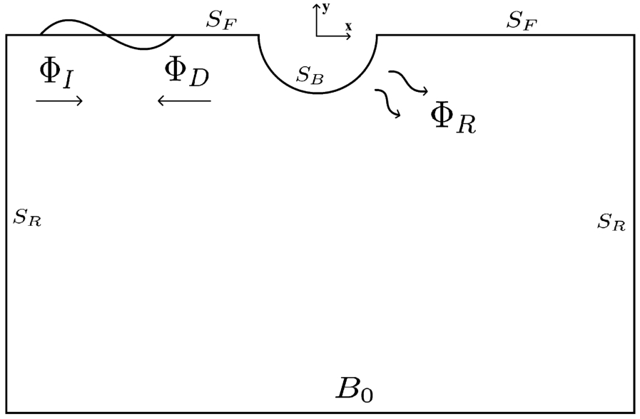
Table 2

List of symbols for components of the total potential and the boundaries of the fluid domain

Abbreviation	Physical meaning
ΦI	Incident wave
ΦD	Diffracted wave
ΦR	Radiated wave
SB	Body surface
SF	Free surface
SR	Radiation boundary
B0	Bottom boundary

At the bottom boundary B0, with position y=−h and h being the water depth, a no-penetration boundary condition is solved

(3)∂Φ∂y=0at y=−h.

A kinematic condition is solved at free surface SF

(4)∂η∂t+∇Φ·∇η=∂Φ∂yat y=η,

with η the free surface. The kinematic condition states that fluid particles at the position of the free surface follow the motion of the free surface.

A highlight of this paper is the generation of waves at radiation boundaries SR. To achieve this, the well-known Sommerfeld radiation condition, also known as absorbing boundary condition (ABC) is changed in to generating absorbing boundary condition (GABC) as in Wellens and Borsboom [13]. The Sommerfeld condition is based on a propagating wave in a certain direction with phase velocity c. At the left radiation boundary, waves that propagate to the left are absorbed; at the right radiation boundary waves that propagate to the right are absorbed. For a wave propagating to the right, at the right-hand radiation boundary, the Sommerfeld condition reads

(5)(∂∂t+c∂∂x)Φ=0.

The wave speed c is defined as ω/k, with ω the wave frequency and k the wave number. In the frequency domain, for a wave mode with argument (ωt−kx), Eq. (5) simplifies to

(6)(∂∂x+ik)Φ=0.

This is also the expression used by Yeung [16] for his radiation problem. For the diffraction problem, the left-hand radiation boundary is also a generation boundary for the incident waves propagating to the right. Following Wellens and Borsboom [13], who derived a GABC for irregular waves in the time domain, the right-hand side of Eq. (6) is given a non-zero value equal to the operators on the left-hand side applied to a wave mode with argument (ωt+kx), yielding a GABC for the frequency domain

(7)(∂∂x−ik)Φ=(∂∂x−ik)ΦI=−2ikΦI

The performance of boundary condition Eq. (7) is demonstrated in Section 4.

2.2.Linear wave theory

It is assumed that the waves are not steep, and are long enough to neglect surface tension. For linear potential flow theory all equations are linearized around y=0, meaning higher than first-order terms are neglected. The kinematic boundary condition then becomes

(8)∂η∂t=∂Φ∂yat y=0.

The atmospheric pressure at the free surface is assumed to be zero

(9)p=0at y=η.

Linearizing the Bernoulli equation, Eq. (2), and substituting Eq. (9), leads to the dynamic free surface boundary condition

(10)∂Φ∂t+gη=0at y=0.

Linear potential flow theory is also known as Airy wave theory. The potential function of an Airy wave

(11)η=Asin(ωt−kx)

that satisfies the fundamental equations and the linearized boundary conditions is

(12)Φ=Agωcosh(k(h+y))cosh(kh)cos(ωt−kx),

with A the amplitude of the Airy wave.

The characteristic equation of the system of equations is the dispersion relation

(13)ω2=kgtanh(kh).

It relates the wave frequency and the wave number. Because c=ω/k, the dispersion relation implies that waves of different frequency propagate at different phase velocities c. The wave length is found from the wave number as L=2π/k and the wave period is found from the wave frequency as T=2π/ω.

2.3.Second-order wave theory

In order to solve the non-linear wave propagation problem, it is common to use perturbation theory. This was first done by Stokes [10] for free surface gravity waves. It was repeated by Newman [8] for waves in infinite water depth. With perturbation theory, a function or solution variable is approximated by a series of terms of increasing order

(14)ξ=ξ(0)+εξ(1)+ε2ξ(2)+⋯

Here, ξ(i) are the expansion terms in the perturbation series approximating solution variable ξ. ε is a small term (for waves it is the wave steepness), so that higher-order terms become smaller as the order increases. An approximate solution is found by truncating the series. From now on, approximated variables are given a superscript (1) or (2) to indicate the order of approximation.

The second-order boundary condition (Stokes [10]) is referred to as the quadratic forcing function (QFF)

(15)−4ωΦ(2)+g∂Φ(2)∂y=QFF,

with

QFF=−∂∂t(∂Φ(1)∂x∂Φ(1)∂x+∂Φ(1)∂y∂Φ(1)∂y)(16)+1g∂Φ(1)∂t∂∂y(∂2Φ(1)∂t2+g∂Φ(1)∂y).

An index to find the non-linearity for waves in finite water depth is the Ursell number

(17)NUrsell=A/L(h/L)3=AL2h3.

It is defined as the steepness/(relative depth)³. The higher the Ursell number, the more non-linear a wave is going to behave. The second-order potential that satisfies the second-order boundary condition at the free surface (Stokes [10]) is

(18)Φ(2)=3A2ω8cosh(2k(h+y))sinh4(kh)sin(2(ωt−kx))

2.4.Pressures and forces

To find the pressures in the domain use is made of the linearized Bernoulli equation

(19)p(1)=−ρ∂Φ(1)∂t−ρgy.

The forces on the body are the integration of the pressures along the body surface Sb, see Fig. 1

(20)F(1)=∫SB(0)p(1)ds.

The buoyancy force on the floating body is found differently. The change in buoyancy in the heave direction is caught by the hydrostatic term in the Bernoulli equation ρgy, in which y is replaced by the vertical position a of the floater. In the presence of waves, the pressure depends on the relative position of the structure with respect to the free surface elevation η−a. The pressure is then integrated over the waterplane area SA

(21)Fb=∫SAρg(η(1)−a(1))ds.

This expression for the buoyancy force is accurate for wall-sided structures and small motions. For non-wall-sided structures it is the zeroth-order approximation. Other motion directions require a similar evaluation.

2.5.Motions

The motions of the floating object are found from an equation of motion for the body. For the vertical direction

(22)ζy=Fy(1)−ω2(M+μ)−iωλ+K,

in which ζy is the response amplitude operator (RAO), defined as the ratio between the body motion amplitude aˆ and the wave amplitude A. M is the body mass, μ the added mass, λ the damping and K the coefficient of the buoyancy. The added mass and damping of the floating body are found from a radiation simulation. The total force on the floater is found from the sum of forces found from a radiation simulation and a diffraction simulation.

2.6.Power prediction & optimal damping

When the floating body is equipped with a generator to harvest wave energy, a power take-off (PTO) device, the power produced can be estimated using the parameters from a BEM simulation. Assume that λPTO is the damping coefficient of the PTO. The produced power as a function of time then becomes

(23)PA(t)=λPTOa˙(t)2.

Velocity a˙(t) is the time derivative of motion a(t) of the body, with aˆ its amplitude.

The average power in one wave period T then becomes

(24a)P‾A=1T∫0TPd(t)dt(24b)P‾A=1T∫0TλPTOω2aˆ2sin2(ωt)dt(24c)P‾A=12λPTOω2aˆ2.

Using RAO ζy with the additional damping λPTO of the generator, an expression for the average power in terms of the damping is found

(25a)ζy=Fy−ω2(M+μ)−iω(λ+λPTO)+K(25b)P‾A=12λPTOω2ζy2A2(25c)P‾A=12λPTOω2A2Fy2(K−ω2(M+μ))2+(ω(λ+λPTO))2.

The optimal damping coefficient λopt of the generator is then found from the expression obtained after taking the derivative of the average power with respect to λPTO and finding its root(s)

(26a)∂P‾A∂λPTO=0(26b)12ω2ζy2Fy2((K−ω2(M+μ))2+ω2(λ2−λPTO2))((K−ω2(M+μ))2+(ω(λ+λPTO))2)2=0(26c)λopt=λPTO=(K/ω−ω(M+μ)2+λ2

2.7.Conservation of energy

Conservation of energy is used to verify the simulations in Section 4. As energy enters and leaves the domain through the radiation boundaries SR in Fig. 1, it is convenient to define dimensionless numbers in terms of the directions of the wave components encountered at those boundaries: the incident wave component, the reflected wave component and the transmitted wave component. Reflection is the combination of diffracted and radiated waves that propagate in opposite direction to the incident wave. Transmission is the combination of incident, diffracted and radiated waves that propagate in the direction of the incident wave. In equations

(27a)R=ΦD−ζyΦRΦI(27b)T=ΦD+ΦI−ζyΦRΦI.

Energy is conserved when the energy flux, or power, that enters the domain, is equal to the power that leaves the domain plus the power that is absorbed by the generator

(28)PI=PR+PT+PA.

Because the incident, reflected and transmitted wave power are related to the incident wave amplitude, the reflected wave amplitude and the transmitted wave amplitude as

(29)PI,R,T=12ρgAI,R,T2ωk,

and because

(30)PA=12λPTOω2ζy2AI2,

energy conservation leads to the following relation

(31)R2+T2+ηh=1,

in which ηh=PA/PI is the efficiency of the power take-off system.

3.Model description

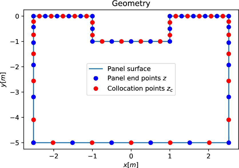
A boundary element method has been adopted to find the hydrodynamic properties of a floating body with an arbitrary geometry and to solve the complete system of motion with both the diffracted as the radiated waves (leading to reflected and transmitted wave components). The choice is made for a method with panels along all boundaries and simple sources instead of Green’s functions, as this will make the extension to second order more feasible. The linear problem is split in a diffraction and a radiation problem, which, when combined, describe the complete equation of motion of the floater. An example of a domain with panels on all boundaries is shown in Fig. 2. The center of each panel features a collocation point.

Fig. 2.

Panel layout.

3.1.Discretization

The approximate solution is achieved by solving a matrix equation for all boundaries simultaneously. Since this is partly a mixed type boundary condition, the potential and the normal velocity must be defined on all panels. The condition is solved for each collocation point (observation point) in the center of each respective panel. Collocation points are points in the fluid along the boundary of the domain, not exactly on the boundary but with a small distance to the boundary to prevent singularities in the integration, see Fig. 3.

Fig. 3.

Panel definitions.

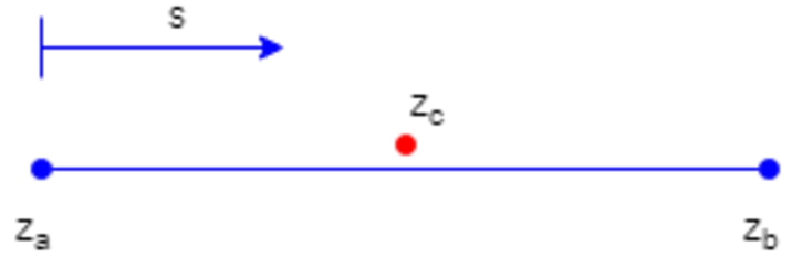
Source panels are used to find the solution to the boundary problem, with sources spread out over the whole panel. The coordinates of the panels are given in the form of a complex vector z

(32)z=x+iy.

Using z, a linear function is created that describes the path s from the start of the panel at za to the end of the panel at zb

(33)z1(s)=za+s(zb−za)

The influence matrix P[m,n] describes the influence of the potential of panel m on panel n. The influence matrix Q[m,n] is used to find the influence of panel m on panel n with regard to the normal velocity of the panel (pointing into the fluid domain)

(34a)P[n,m]=∫panell[n]2πln(zc[m]−z1[n](s))ds(34b)Q[n,m]=∫panell[n]2π∂∂npln(zc[m]−z1[n](s))ds

Here, l is a vector containing the lengths of panels.

The influence matrices can pose a challenge. A numerical approach is taken to find the potential value influence matrix P[m,n] and the normal velocity influence matrix Q[m,n]. The matrices are found by numerical integration of sources along each panel. The challenge arises when m=n. At this panel, the collocation point zc is very close to the panel surface. If the integration step is not small enough, integration errors will occur on this panel as the distance between the panel and the collocation point is critical in the result. To ensure a good result, the integration step size has been reduced until the solution converges.

Linear boundary condition matrices

With these descriptions of the normal velocities and potential in the entire domain, the boundary conditions can be written in a discretized form. To solve for all boundaries simultaneously, the problem must be brought into a single matrix equation.

(35)C[n,m](1)=Q[n,m]−ikP[n,m],n∈SLQ[n,m],n∈SbQ[n,m]+kP[n,m],n∈SFQ[n,m]−ikP[n,m],n∈SRQ[n,m],n∈B0

This matrix C contains all influence matrices that need to be solved for. Another matrix, describing the known behaviour of the fluid at its boundaries is also determined. This matrix is different for the diffraction problem and the radiation problem.

Diffraction problem:

(36)K[n](1)=−2ikΦ(1),n∈SL0,n∈Sb0,n∈SF0,n∈SR0,n∈B0

Radiation problem:

(37)K[n](1)=0,n∈SLa˙n[n](1),n∈Sb0,n∈SF0,n∈SR0,n∈B0

with a˙n[n] the normal body velocities

(38)a˙n[n]=nb[n]·ub[n].

The source strengths q[n] are found as the solution of

(39)C[n,m](1)q[n](1)=K[n](1).

And from the resulting source strengths, the potential and the free surface values are reconstructed

(40a)Φ[n](1)=P[n,m](1)q[n](1)(40b)η[n](1)=−iωgΦ[n](1)for n∈SF

Second-order boundary condition matrices

To find the second-order results, a new influence matrix G is created. This matrix replaces the Q[m,n] matrix in finding the derivatives of the potential in y.

(41)G[n,m]=∂∂yP[n,m]=2ktanh(2k(h+y))P[n,m]

The tanh(2k(h+y)) term originates from the transformation of the cosh(2k(h+y)) to a sinh(2k(h+y)) when taking the partial derivative in y. This matrix can only be used for a propagating wave without a floating body in the domain, because this use of the derivative is not valid for evanescent waves near the floating body. The complete influence matrix becomes

(42)C[n,m](2)=gG[n,m]−4ω2P[n,m],n∈SFG[n,m],n∈B0

Since the presented solution does not contain a body, the right-hand side is given by

(43)K[n](2)=QFF[n],n∈SF0,n∈B0,

after which the source strengths are solved from

(44)C[n,m](2)q[n](2)=K[n](2).

4.Results

The implemention of the method is verified by means of first-order simulations with a floating cylinder featuring a power take-off device (PTO) and second-order simulations of a propagating free surface wave.

4.1.First-order results with a floating body

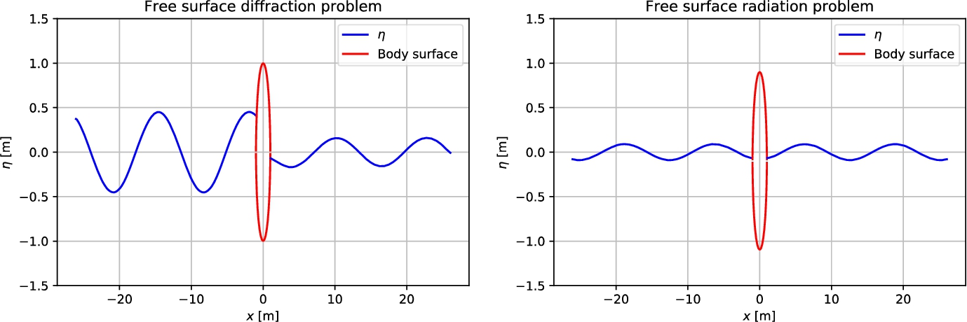
The vertical motion of a floating cylinder with a circular cross section and radius R=1 m in waves is considered. The domain has a size of 25m on either side of the cylinder and a depth of 100 m. The panel size was taken to be 0.52 m, so that twelve panels fit the circumference of the cylinder and 100 panels fit the free surface in horizontal direction on either side of the cylinder. In depth direction, the size of the panels grows exponentially with each panel in downward direction being 2% larger than the panel above it. Diffraction problems with multiple wave frequencies are considered with unit wave height. Radiation problems are simulated for those same frequencies with unit vertical velocity of the floater. Figure 4 shows free surface of the diffraction simulation and the radiation simulation for a wave propagating to the right with a wave frequency of 2.3 rad/s. The diffraction problem features the incident wave component (propagating to the right) and the reflected (diffracted) wave component (propagating to the left) on the left of the cylinder, forming a partial standing wave system. Without a functional GABC at the left boundary of the domain, the wave height to the left of the cylinder would not have a finite value. The right side of the cylinder features a transmitted wave component, which is the combination of the incident wave component and the diffracted wave component. In the radiation problem, the wave components on either side propagate away from the heaving cylinder. The wave component on the left of the cylinder adds to the reflection, the wave component on the right adds to the transmission.

Fig. 4.

Wave profiles with body for the diffraction problem and for the radiation problem.

$Wave profiles with body for the diffraction problem and for the radiation problem.$

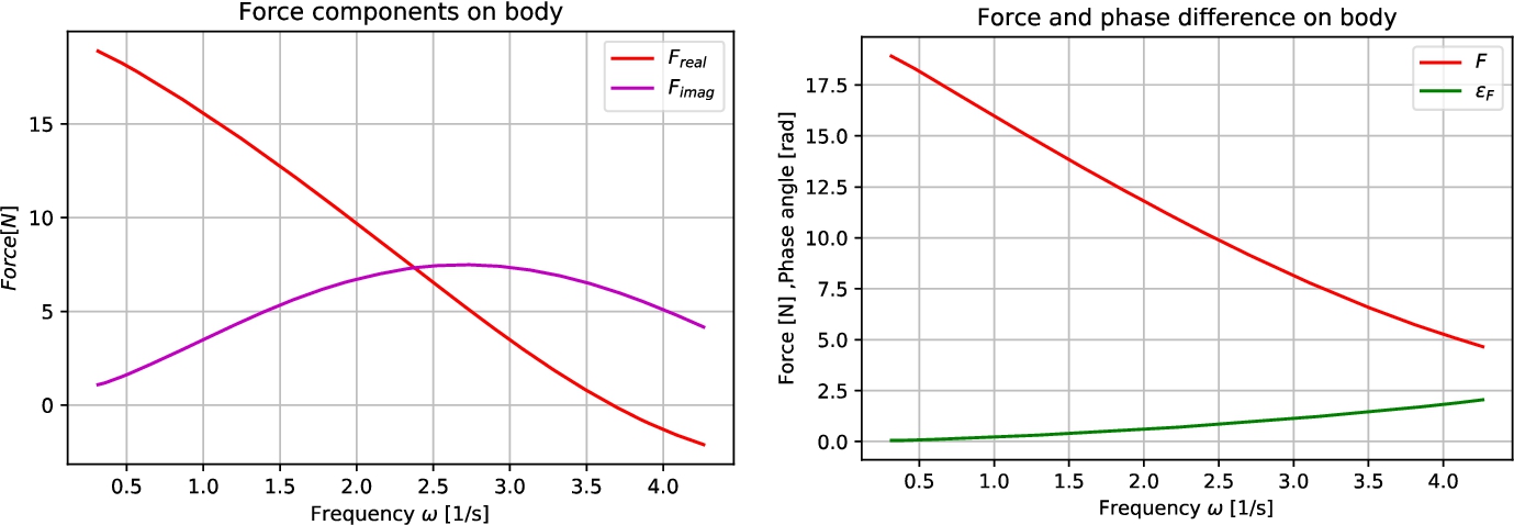
Diffraction force

The vertical force on the cylinder is found from the discrete potential that is reconstructed from the vector of source strengths

(45)Fy=iρω∑nΦ[n](1)s[n]nb,y[n]for n∈Sb,

in which s[n] is the vector with panel sizes and nb,y[n]j the projection of the panel’s normal vector on the y-axis.

For the diffraction problem, the vertical force is shown in Fig. 5. The panel on the left of the figure shows the real part Re(Fy) and imaginary part Im(Fy) of the vertical force. The panel on the right of the figure shows the force amplitude |Fy| and the phase tan−1(Im(Fy)/Re(Fy) of the force with respect to the wave.

Fig. 5.

Diffraction force on a cylinder in heave.

$Diffraction force on a cylinder in heave.$

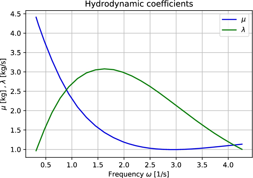
Radiation force

For the radiation problem, the vertical force is determined in the same way as in Eq. (45). From that force, the added mass coefficient μ is found from the part of the force in phase with the motion

(46)μ=−Re(Fy)ω2aˆ.

The damping coefficient λ is found as the part of the vertical force out of phase with the motion

(47)λ=Im(Fy)ωaˆ.

The added mass and damping for the floating cylinder are shown as a function of frequency in Fig. 6.

Fig. 6.

μ and λ for a cylinder in heave.

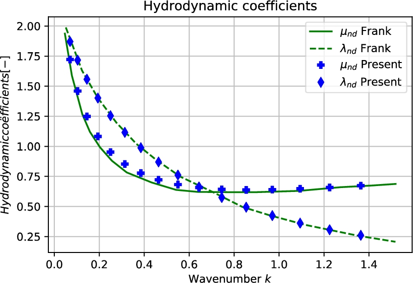
When the added mass and damping are made non-dimensional in a way similar to Yeung [16] as μnd=μ/0.5ρR2 and λnd=λ/0.5ρωR2, their values can be compared to existing literature. The non-dimensional values for the added mass and damping are shown in Fig. 7, where they are compared with the results of Frank [4].

Fig. 7.

Verification hydrodynamic coefficients.

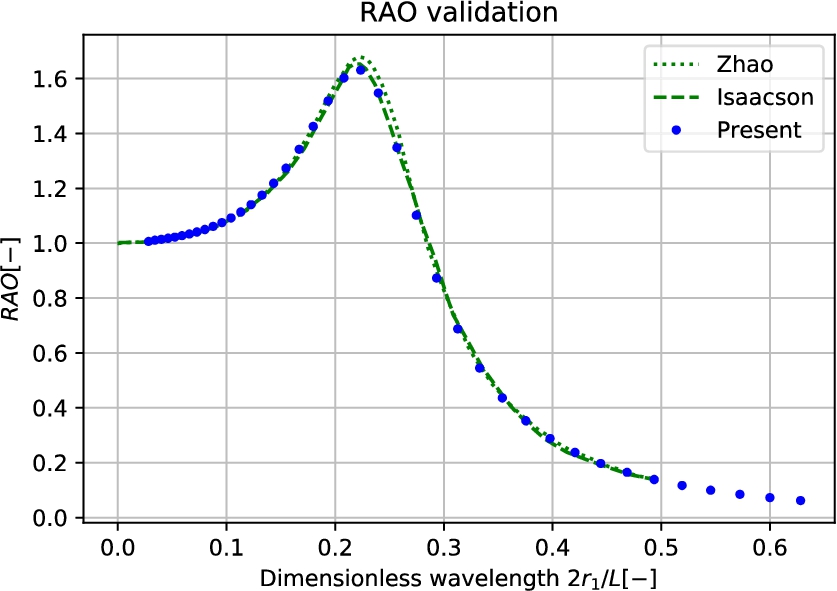
Equation of motion

The forces from the diffraction problem and the coefficients from the radiation problem are combined with the buoyancy of the floating cylinder in Eq. (21) and the mass M=0.5ρπR2 to determine the RAO according to Eq. (25a). At first, a value of λPTO=0 is used as if no PTO device is present. The RAO as a function of one over the wave length, made non-dimensional with the diameter of the cylinder, is shown in Fig. 8, where it is compared to the results of Zhao et al. [17] and Isaacson and Baldwin [5]. The differences with Zhao et al. [17] are small. They are just as small as the differences between Zhao et al. [17] and Isaacson and Baldwin [5] and due to discretization errors.

Fig. 8.

RAO results.

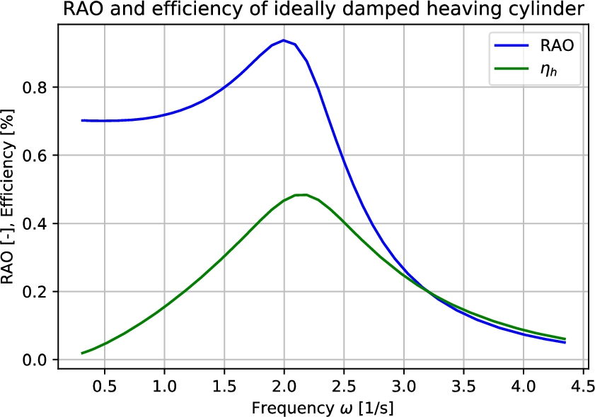
With a PTO device, and a PTO damping λPTO=λopt, see Eq. (26c), the RAO – now as a function of frequency – becomes as it is depicted in Fig. 9. The additional damping of the PTO reduces the motion response of the floater. In the same figure that contains the RAO with PTO damping, the efficiency ηh of the PTO device is plotted. One can tell that, as expected from the derivation in Eq. (26c), the efficiency peaks near the natural frequency of the floater.

Fig. 9.

RAO and efficiency of ideally damped heaving cylinder.

Energy conservation

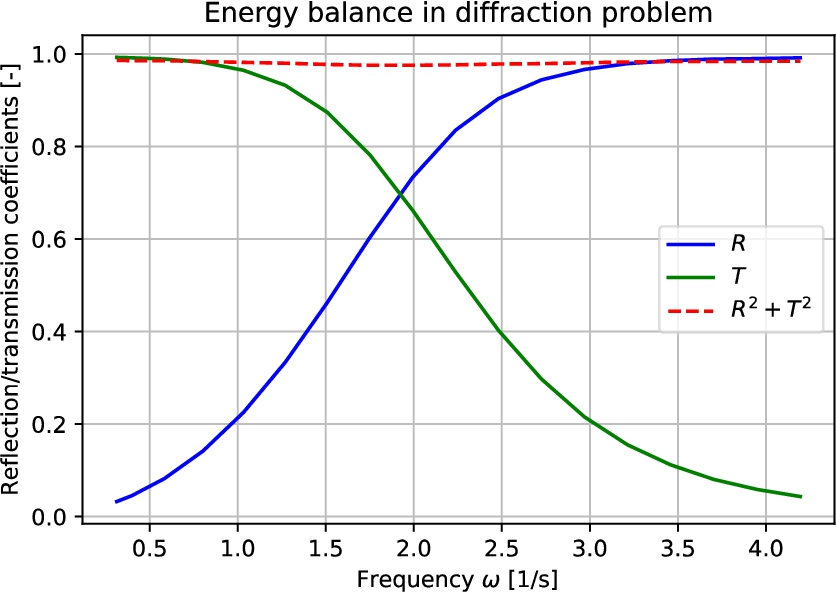
The results of the heaving cylinder with ideal damping according to the equations in Section 2.7 are plotted in Fig. 10 and Fig. 11. Figure 10 shows the radiation coefficient R and the transmission coefficient (T) from the simulation with incoming waves, radiation and diffraction. Energy is conserved when R2+T2=1. The figure demonstrates that this is very nearly the case, apart from a region of frequencies near the natural frequency of the floater. Near that region, the radiated waves have the most influence on the reflection coefficient and the transmission coefficient. Because there is a discretization error in the representation of the wave length (and hence phase velocity of the wave), the effect of the discretization error on R, T and R2+T2 is largest in the region near the natural frequency of the floater.

Fig. 10.

Radiation and transmission coefficients and energy conservation.

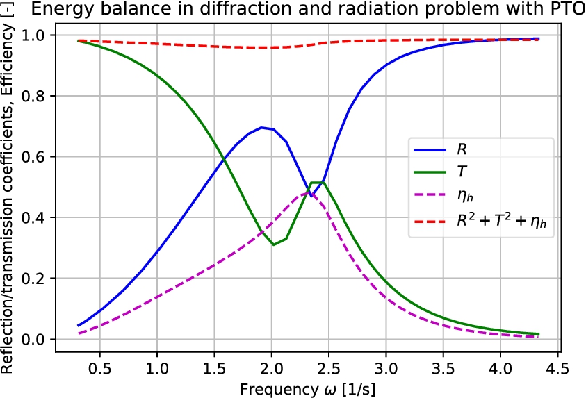
The results with power-takeoff (PTO) device on the floater are shown in Fig. 11. It gives the reflection coefficient, the transmission coefficient, the efficiency of the power-takeoff and the total energy flux to and from the system. As can be seen, hardly any energy is lost to the system, apart from the region of frequencies near the natural frequency of the floater. This verifies the results for first-order simulations with a PTO present.

Fig. 11.

Energy conservation with PTO.

4.2.Second-order results for a propagating wave

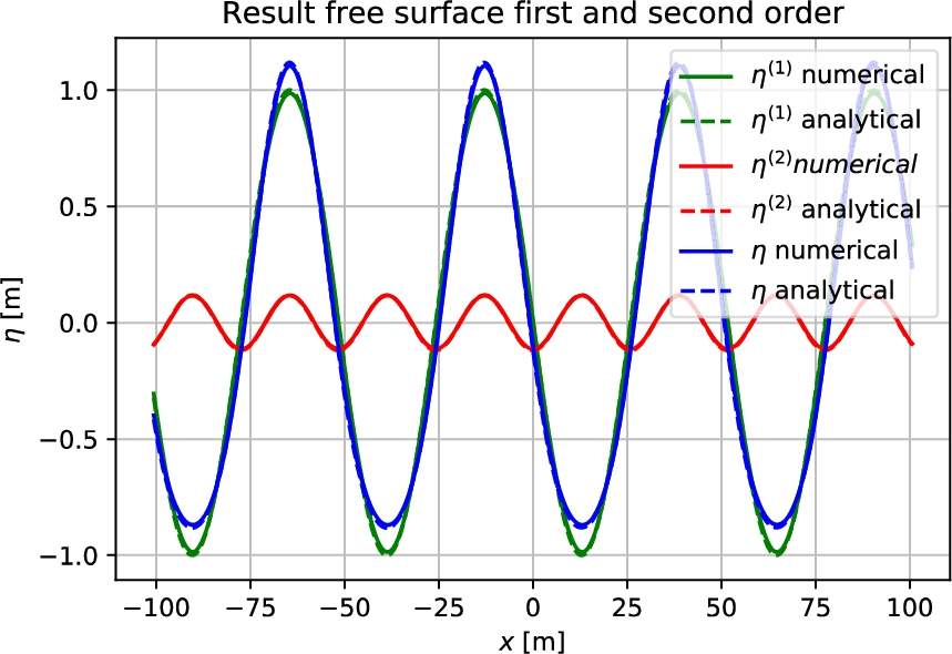
Panels were placed along all boundaries of the simulation domain – instead of only along the boundary of the floater as in many BEM implementations (Frank [4]) – so that second-order simulations would be possible. A second-order propagating wave is simulated. The wave height was 2 m, the wave period was 5.6 s. The water depth was chosen to be 100 m. The panel size was 1 m so that approximately 100 panels were used per wave length. The size of the panels in vertical direction starts out at 1 m, but increases exponentially in vertical direction with each panel further down 2% larger than the panel above it. The linear and second order results for a propagating wave generated with a GABC on the left and an ABC on the right are shown in Fig. 12. These are compared to the analytical relations given above. It is shown that the first and second-order components of the total surface elevation are a good match with the analytical solution.

Fig. 12.

First and second-order wave surface elevation.

5.Conclusions

A novel boundary element method is developed with panels at all domain boundaries and a straightforward Green’s function so that extension to second order is feasible. Simulations are performed in the frequency domain. The diffraction problem with incident waves is solved in one part of the method, the radiation problem in another. A generating and absorbing boundary condition for the side walls of the domain was derived and implemented to make the combination of incident and diffraction waves at the same boundary possible. The following conclusions are found:

1. Added mass and damping found from the radiation problem are nearly the same as those of Frank [4].
2. The response amplitude operator found from the combination of two simulations, one with incident waves and diffraction, and one with radiation, closely resembles those in earlier literature.
3. Without a power take-off device, energy is nearly conserved in the combined incoming wave, diffraction and radiation problem. Energy is not conserved perfectly due to discretization errors.
4. With a power take-off device, tuned for optimal damping at the natural frequency of the floating body, the energy lost to the floating system is nearly equal to the energy taken up by the power-takeoff device. The small difference is the result of discretization errors.
5. Following the verification with second-order wave propagation, the model is suitable for extension to second order.
6. In first-order and second-order simulations, the GABC and ABC at the left and right radiation boundaries function according to theory.

Funding

The authors report no funding.

Conflict of Interest

Peter Wellens is an Editorial Board Members of this journal, but was not involved in the peer-review process nor had access to any information regarding its peer-review.

Author contributions

Maarten Gabriel: Conceptualization, Methodology, Formal analysis, Investigation, Visualization, Writing – original draft. Peter Wellens: Conceptualization, Writing – review and editing, Supervision

References

[1]	A. Ballast, Water Waves, Fixed Cylinders and floating Spheres, 2004, p. 302. ISBN 9064648956.
[2]	R.W. Bos, M.v.d Eijk, J.H. Besten and P.R. Wellens, A reduced order model for FSI of tank walls subject to wave impacts during slosing, International Shipbuilding Progress 69 (2022).
[3]	W.R. Dean, On the reflexion of surface waves by a submerged plane barrier, Mathematical Proceedings of the Cambridge Philosophical Society 41: (3) ((1948) ), 231–238. doi:10.1017/S030500410002260X.
[4]	W. Frank, Oscillations of Cylinders in or Below the Free Surface of Deep Fluids, (1967) .
[5]	M. Isaacson and J. Baldwin, Wave Propagation Past a Pile-Restrained Floating Breakwater 8(4) (1998), 1–5.
[6]	M. Kim and D.K. Yue, The complete second-order diffraction solution for an axisymmetric body. Part 2. Bichromatic incident waves and body motions, Journal of Fluid Mechanics 211: ((1990) ), 557–593. doi:10.1017/S0022112090001690.
[7]	Y. Kim, S.H. Kim and T. Lucas, Advanced Panel Method for Ship Wave Inviscid Flow Theory (SWIFT), (1989) .
[8]	J.N. Newman, Marine Hydrodynamics – Waves and Wave Effects (Ch. 6), Marine hydrodynamics (1977), 237–327. ISBN 978-0-262-14026-3.
[9]	T.F. Ogilvie, First- and second-order forces on a cylinder submerged under a free surface, Journal of Fluid Mechanics 16: (3) ((1963) ), 451–472. doi:10.1017/S0022112063000896.
[10]	G.G. Stokes, On the theory of oscilatory waves, Mathematical and Physical Papers 1: ((1847) ), 225–228. ISBN 0521419662. doi:10.1017/CBO9780511702242.016.
[11]	F. Ursell, On the Heaving Motion of a Circular Cylinder on the Surface of a Fluid, April 1948, 1949.
[12]	F. Ursell and W.R. Dean, Surface waves on deep water in the presence of a submerged circular cylinder, Mathematical Proceedings of the Cambridge Philosophical Society 46: (01) ((1950) ), 153. doi:10.1017/S0305004100025573.
[13]	P.R. Wellens and M. Borsboom, A generating and absorbing boundary condition for dispersive waves in detailed simulations of free-surface flow interaction with marine structures, Computers and Fluids (2019), 104387. doi:10.1016/j.compfluid.2019.104387.
[14]	P. Xu and P.R. Wellens, Fully nonlinear hydroelastic modeling and analytic solution of large-scale floating photovoltaics in waves, Journal of Fluids and Structures 109: ((2022) ), 103446. doi:10.1016/j.jfluidstructs.2021.103446.
[15]	P. Xu and P.R. Wellens, Theoretical analysis of nonlinear fluid–structure interaction between large-scale polymer offshore floating photovoltaics and waves, Ocean Engineering 249: ((2022) ), 110829. doi:10.1016/j.oceaneng.2022.110829.
[16]	R.W. Yeung, A singularity-distribution method for free surface flow problems with an oscillating body, 1973.
[17]	X. Zhao, D. Ning, C. Zhang and H. Kang, Hydrodynamic investigation of an oscillating buoy wave energy converter integrated into a pile-restrained floating breakwater, Energies 10(5) (2017). ISBN 8641184708. doi:10.3390/en10050712.