
Exploring the limits of RANS-VoF modelling for air cavity flows
Abstract
Background:
Air lubrication techniques have the potential to significantly reduce frictional drag, benefiting sustainable employability of ships. However, these techniques are not yet widely applied in the shipping industry, since a complete understanding of the relevant two-phase flow physics is still lacking.
Objective:
This article aims to explore the limitations and capabilities of RANS-VoF modelling to numerically model air cavity flows.
Methods:
Simulations were performed including numerical uncertainty verification and compared to experimental data for an external cavity. To study the effect of reduced eddy-viscosity at the cavity interface, two types of eddy-viscosity correction functions were applied next to a base case, i.e., a power and a Gaussian function.
Results:
The cavity length and thickness as well as the velocity profiles in the boundary layer just upstream, in the middle and downstream of the external cavity compare well to experimental data. However, in contrast to what was found experimentally, a too strong coupling was found between the computed cavity profile and the air pressure at the nozzle and too much air leaks out of the cavity. For the same nozzle air pressure as in the experiments, similar cavity dimensions were found, but the air flow rate is overestimated by a factor of five.
Conclusions:
The used methodology is capable of predicting the cavity profile and velocity profiles at different stream-wise locations in the boundary layer around the cavity with respect to experimental findings. However, a mismatch was found in the determination of the required air flow rate for the cavity, which is hypotesized to be mainly caused by the incorrect turbulence modelling around the interface and the advection of a smeared air-water interface in the reattachment zone. This is a direct consequence of the used VoF method. The exact mechanism for air discharge at the cavity closure is still not clear.
1.Introduction
1.1.Background and relevance
In a constant search for techniques to reduce a ship’s total power consumption, air lubrication techniques have shown great potential in reducing a ship’s frictional drag. Air lubrication techniques have realised total propulsive power reduction percentages of 10–20% (e.g. [1–3]) and could possibly realise pollution reduction percentages in the same order of magnitude. However, the physics involved with these flows are not yet completely understood, holding back the application of air lubrication techniques in practical ship design.
Flows around air lubricated ships can be described by two flow regimes where air is distributed in water: the dispersed flow regime and the stratified flow regime. The dispersed regime is characterised by the liquid around the body being saturated with gas bubbles and is also referred to as the bubble drag reduction technique.
The current research focuses on the stratified flow regime which is entered when the surface underneath the ship’s hull is covered by a sustained gas layer. The liquid phase is completely replaced by the gas phase, thus decreasing the ship’s wetted area. This is the most attractive flow regime when aiming for frictional drag reduction since the local wall friction of a submersed body is defined by the viscosity, density and the velocity gradient in the boundary layer and the stratified air layer beneath the ship’s hull gives the largest reduction in both the local density and molecular viscosity. The flow regimes of interest for typical cargo ships at full scale are characterised by relatively low Froude (
Fig. 1.
Drag reduction techniques in the stratified flow regime: air layer (a), external air cavity (b) and internal air cavity (c).
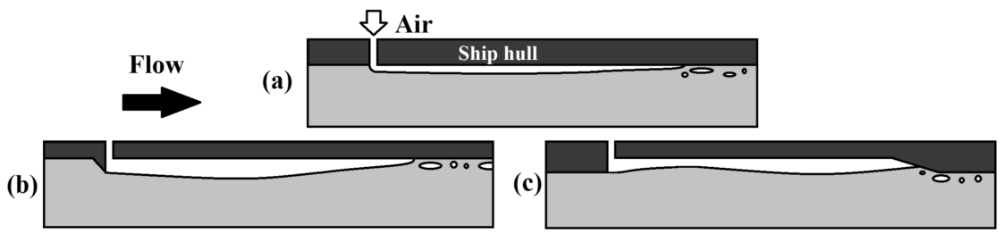
1.2.External air cavities
When a small ‘cavitator’ is applied directly upstream of a point of air injection, an external cavity can be created (Fig. 1(b)). The cavitator creates a suction pressure directly downstream of it, separating the mean flow from the wall. The pressure disturbance together with the density difference causes a difference in inertia, and thus a gravity-induced surface wave. This wave describes a stable air cavity, with a length prescribed by half the wavelength λ of the surface wave. Here, it is assumed that the celerity of the wave is equal to the ship’s speed, looking at the cavity underneath the ship in a moving frame of reference. This model is described by e.g., Butuzov [4], Matveev [5] and Ceccio [6]. Zverkhovskyi [2] shows experimentally that the cavity length is a function of the depth-based Froude number in the Delft cavitation tunnel. It can be found through the dispersion relation which is given by Eq. (1), where
1.3.Cavity stability and air loss mechanisms
The reported possible total propulsive power reductions of 10–20% seem very promising, but air lubrication techniques are not yet widely applied due to a lack of understanding of the sensitivity of the air layers to overall hull shape. The largest challenge in predicting the air cavity characteristics lies in the full scale prediction of the cavity stability and required total air supply, which determines the total power reduction, operability and safety of the complete air lubrication system.
Zverkhovskyi [2] found that the shallow-water effect can substantially increase the cavity length for external air cavities, since the wavelength is also a function of the water depth. Also, the cavity length and thickness can somewhat be influenced by the initial flow conditions such as the boundary layer thickness and angle of attack of the surface where the cavity is created with respect to the incoming flow. Mäkiharju [3] reports experimental work on air cavities where it was found that the gas flux needed to establish the cavity is higher than the flux needed to maintain the cavity. The required air flux in steady flow is a function of Froude number, Reynolds number, Weber number and closure geometry.
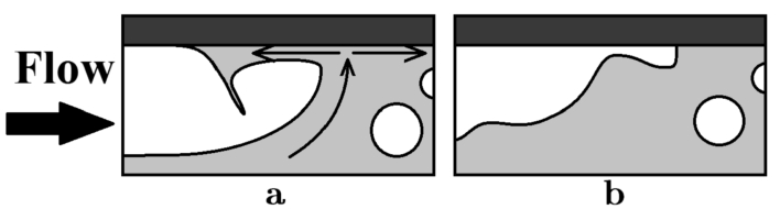
Focussing more on the different air loss mechanisms for air cavities, most of the published work is of experimental nature. Two different air loss mechanisms (closure mechanisms) are described, the first is the re-entrant jet mechanism (Fig. 2(a)) and the second one is the wave pinch-off mechanism (Fig. 2(b)) (e.g. [2,7–10]). The contribution of each of these mechanisms depends on the flow conditions (flow velocity, turbulence intensity) and geometry of the cavity.
The re-entrant jet mechanism for an air filled cavity is provisionally assumed to be similar to the re-entrant jet mechanism responsible for the break-up of vapour sheet cavities as described by Callenaere et al. [11]. In the closure region of a sheet cavity, a region with high adverse pressure gradient is formed. The increase in local pressure forces a thin stream of liquid into the cavity, which is called the re-entrant jet. It is the fluid between the dividing streamline and the cavity, and it tends to fill the cavity. However, in the case of an air cavity, the smaller pressure gradient, flow velocities, viscous effects, and the direction of gravity prevent the liquid jet from reaching the far upstream part of the cavity. It loses its momentum and falls. Impingement of the jet with the gas-liquid interface results in that a portion of the attached cavity is being pinched off and transported by the mean flow. The cavity then grows and the shedding cycle starts again. It results in a periodic behaviour which is dynamically stable. Here, the re-entrant jet does thus not exist continually. For the external air cavity, it is hypothesized that this mechanism is only present when the cavity is still developing, and when the cavity is relatively thick in comparison to its length, so that the adverse pressure gradient in the closure gradient is high enough to force a stream of liquid inside.
The wave pinch-off mechanism is governed by waves on the air-water interface. Their wavelengths are in the order of 0.5–2 cm for model scales [3]. These waves are believed to be formed by turbulence structures originating form the turbulent boundary layer upstream of the cavity, which disturb the free surface. If the resulting wave amplitudes are of the same magnitude as the cavity thickness, the free surface interface hits the ship bottom and a pocket of air is shed from the cavity.
Fig. 2.
Air loss mechanisms for the internal and external air cavity. Re-entrant jet mechanism (a) and wave pinch-off mechanism (b).
1.4.Numerical modelling of air cavity flows
Multiphase computational fluid dynamics (CFD) methods could help in providing a better understanding of the sensitivity of the air layers to overall hull shape and the flow parameters. It can also provide a tool to predict the total propulsive power requirements and operability profile in the early design stage of air lubricated ships. From a practical point of view, this means that only potential flow solvers and viscous flow solvers which are capable of solving two-phase flows are of interest.
The global flow pattern around cavities can be analyzed with linearized potential flow theory, where the relation of the mean parameters such as pressure, length and thickness of a cavity are computed [4,5]. Several viscous flow simulations for air cavities are reported [8,12,13], where the most important finding is that the key to the numerical prediction of the air layer characteristics lies in the correct modelling of the closure region. Menon et al. [12] focused on influence of the Volume of Fluid (VoF) interface capturing scheme used to model the air-water interface. It was found that the wave profile formed inside the cavity was influenced when more compressive schemes are used for the discretization of the free-surface transport equation. Zverkhovskyi [13] reported that when the shape of the free surface of a cavity is known a-priori, it can be modelled using a slip wall and the shear stress around the artificial cavity can be correctly computed using a single-phase flow approach. However, the cavity surface in the region of the closure is highly unstable and unknown. Furthermore, to be able to compute the required air flux, a two phase flow approach is needed. For internal cavities, the cavity surface from the step up to just before the closure region could correctly be modelled using a VoF approach, but the amount of air leakage from the closure of the cavity could not be modelled correctly. Lastly, it was concluded that to enhance the stability of the air pressure inside the cavity and the cavity profile itself, it is required to specify a boundary condition with a constant nozzle pressure instead of a constant volume flux.
More demanding models such as Large Eddy Simulation (LES) and Direct Numerical Simulation (DNS) can also be used to identify the physical conditions in the closure region and to study and identify scaling influences. Kim and Moin [14] reported on an air layer computation using direct numerical simulation (DNS). The air layer is created using a backward facing step (similar to the internal air cavity technique) but there is no beach geometry applied to the problem and the air layer is significantly thicker than the air layers and cavities studied in this research, especially in the closure region. For the break-up of the air layer, a Kelvin-Helmholtz instability is reported when the air supply to the air layer is lowered. Two exploratory studies for setting up scale resolving simulations for the external cavity case are reported in [15,16].
1.5.Objectives and scope
This article aims to investigate the limitations and possibilities of using a RANS-VoF approach to numerically model the flow around an air lubricated surface. More demanding models such as LES are outside the scope of this article. We aim to link the physical modelling of the relevant physical phenomena to their numerical modelling, with an emphasis on the modelling of the re-entrant jet mechanism for the external cavity. The wave pinch-off mechanism will be excluded from this article, since it is known a-priori that a pure RANS approach is not capable of computing the turbulence structures that are believed to be responsible for disturbing the cavity surface. This article is an extension of earlier work on RANS simulations for air cavities, for which is referred to Rotte el al. [17–19].
The numerical solver used for all simulations is ReFRESCO [20]. It is a multiphase (unsteady) incompressible viscous flow solver using the RANS equations, complemented with turbulence models. The available turbulence closure includes the commonly used (U)RANS models and Scale-Resolving Simulations (SRS) models such as DDES, XLES and PANS. Time integration is performed implicitly with first or second-order backward schemes.
2.Methods
2.1.Numerical settings and computational grids
The (2D) simulations for the air cavities are based on the dimensions of the Delft Cavitation Tunnel. The work by Zverkhovskyi [2] provides experimental data from this facility for the external cavity case. The cavitation tunnel has a test section length of 2 m and a
A schematic of the computational domain including the applied boundary conditions is shown in Fig. 3. The hydrostatic pressure is kept constant at the bottom. On both sides a symmetry boundary condition is applied. The close-ups in Fig. 3 show the grid topology in the region including the cavity, with refinement zones in the region around the cavitator with height
Fig. 3.
Computational domain and grid for the external cavity computations. The close-ups show the grid topology in the region including the cavity (right close-up) and around the cavitator with height
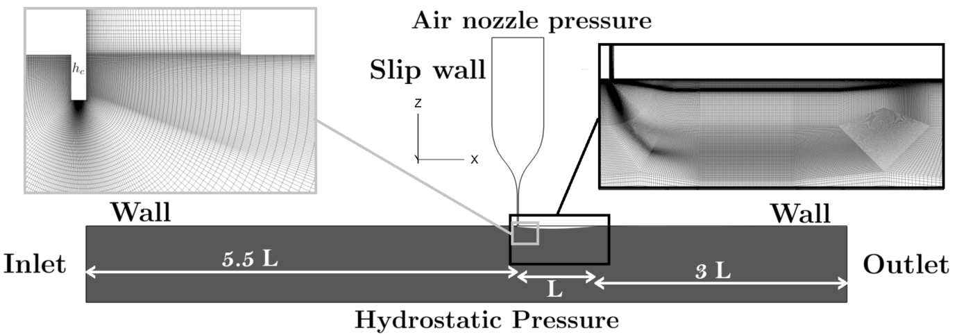
Table 1 gives an overview of the main flow conditions and dimensionless parameters relevant for the problem. The length scales used for the determination of the dimensionless parameters are the cavity length L, the depth of the channel D, the upstream flat plate distance x and the height of the cavitator h. At the simulated flow velocity, the depth-based Froude number
Table 1
Main flow conditions
| 0.56 | |
| 0.58 | |
| 20.8 |
Unsteady simulations were carried out with a water tunnel inlet velocity of 1 m/s. Based on recent experimental observations in the Delft Cavitation Tunnel, this is the free-stream velocity at which the re-entrant jet mechanism is dominant over the wave pinch-off mechanism. All computations were carried out using the
2.2.Cavity profile evaluation
Zverkhovskyi et al. [13] found non-physical air cavity solutions if the air nozzle inlet was prescribed by a constant velocity boundary condition. Instead of having a constant volume flux it is better to define the pressure at the nozzle inlet. To determine the sensitivity of the cavity profile to the prescribed pressure, simulations with air inlet pressures of 10, 15, 20, 25 and 30 Pa were carried out on Grid 3 (Section 2.4, Table 2) with timestep
Fig. 4.
External air cavity profiles and their sensitivity to the prescribed pressure at the air inlet boundary. Flow from left to right.
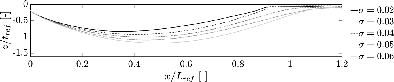
Based on this pressure sensitivity analysis for the cavity profile, the prescribed pressure at the air inlet for the remainder of the simulations and analysis for the air cavity was chosen such that the cavity dimensions from the simulations match the dimensions from the experiment as close as possible. This resulted in a nozzle pressure of 20 Pa (
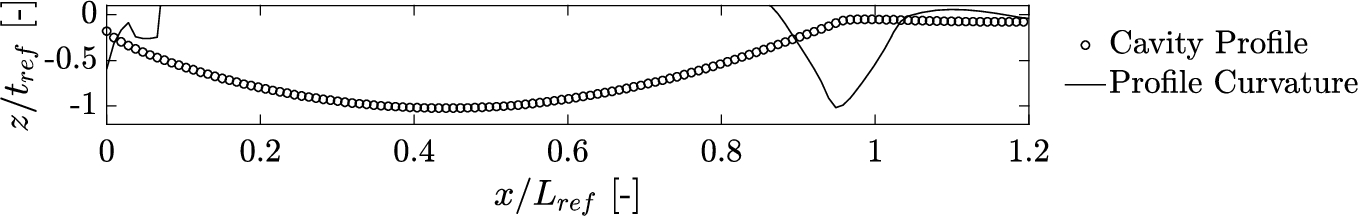
Fig. 5.
Determination of the cavity length based on the absolute maximum of the cavity profile curvature. Flow from left to right.
2.3.Eddy-viscosity correction
For the numerical modelling of the re-entrant jet in the air cavity cases, it is questionable whether RANS methods can directly be used. These turbulence models generally do not predict well large separation areas, the eddy-viscosity near the cavity interface will smooth the interface motions and the cavity problem is inherently a dynamic problem, so the use of time-averaged RANS models is questionable. However, for the simulation of unsteady vapour sheet cavity dynamics, and in particular the re-entrant jet mechanism occurring in those cases, RANS methods are already applied including empirical-based cavitation models. The commonly used two-equation turbulence models, such as the
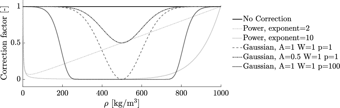
Computations for the air cavity were carried out with the standard KSKL turbulence model as well as applying two different eddy-viscosity correction functions: a power function as used by Reboud et al. [23] and described in Coutier-Delgosha et al. [25] and a Gaussian function which is proposed in [18]. In these cases, the originally computed eddy-viscosity
The Gaussian function is controlled by A and W, which are the amplitude and width of the distribution and have a value between 0 and 1. The order of the function is controlled by p and also has an influence on the width of the peak.
Figure 6 shows the behaviour of the correction functions for different values of power exponent n for cases of the power correction function and different values of A, W and p for Gaussian correction cases. The power function is asymmetrical and has a strong bias towards the lower density fluid. It also has large gradients when the mixture approaches pure air or pure water, which can possibly introduce numerical difficulties. The Gaussian function is symmetric over the interface. For more information on these eddy-viscosity correction models reference is made to [23,25] and [18].
Fig. 6.
Eddy-viscosity correction factors following from the power function and Gaussian function as a function of the local density ρ. The computed eddy-viscosity is multiplied by this correction factor. 0: full reduction of the computed eddy-viscosity, 1: no reduction of the computed eddy-viscosity.
2.4.Numerical uncertainty estimation
To assess the numerical uncertainty in the simulations, a distinction is made between the round-off error, the iterative error, the discretization error and, in case of unsteady simulations, the statistical error. The round-off error is a consequence of the finite precision of computers. Its importance tends to increase with grid refinement, but the error is usually negligible compared to the other sources of error due to double-precision arithmetic [26,27].
The iterative error can theoretically be brought down to machine accuracy levels, but this in terms of computational costs this is not always feasible or achievable for industrial problems [26]. Regarding the iterative convergence of all the simulations presented; the
The discretization error is caused by the approximations made by discretizing the partial differential equations and the finite resolution of the grid. For the assessment of the discretization error, the methods as described by Rosetti et al. [28] and Eça and Hoekstra [27] are followed, which are based on grid and time step refinement.
A least squares fit on the data is made based on a power series expansion with 1st and 2nd order terms. The quality of the fit is then determined using the standard deviation of the fit, and depending on this quality a safety factor is selected and the discretization uncertainty is estimated. Due to the spatial and temporal dependency of the fit, the solution could be visualized by a three-dimensional surface.
Four different grids and three different time step sizes were used for the air cavity simulations (Table 2). Here, the
To verify the stationarity of the signal, and to estimate the start-up effects in the results, the Transient Scanning Technique (TST) as described by Brouwer et al. [29] is applied. This information is used to identify the start-up effects and to remove them from the signal in order to determine the mean more accurately. The TST was applied for cavity length, thickness and required air flux.
Table 2
Grids and Courant numbers for the discretization uncertainty estimation. The three time steps used are
| Grid | # cells | ||||
| 4 | 2 | 1.5 | 3 | 15 | |
| 3 | 1.5 | 2 | 4 | 20 | |
| 2 | 1.2 | 2.5 | 5 | 25 | |
| 1 | 1 | 3.0 | 6 | 30 |
3.Results
3.1.Numerical uncertainties
Regarding the numerical uncertainty of the simulations, the main focus is on the discretization error. Figure 7 shows the signal for the computed air flux through the nozzle over time for the first seven seconds as computed on the finest grid. The mean air flux as computed on the same grid is more or less the same for every time step used, and this also holds for the computed mean length and thickness of the cavity. Due to time considerations, the simulations were only continued for the largest time step of 5 ms on all grids, assuming that the mean values for length, thickness and air consumption are independent of the applied time step size. Figure 7 also shows a periodic behaviour of the required air flux. This periodic behaviour dampens out on all grids but the finest grid and the air flow converges to a steady solution.
Fig. 7.
Signal for the air flow rate in time for the first 6 seconds simulation time as computed on the finest grid for all three time steps.
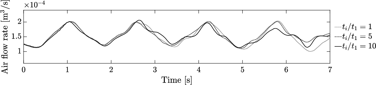
Table 3 shows the values for the spatial discretization uncertainty for the mean cavity length, thickness and required air flow rate as estimated for every grid. Here,
Table 3
Discretization uncertainty estimation for every grid
| Item | p | ||||
| 1.00 | 1.2% | ||||
| 1.20 | 1.4% | ||||
| 1.50 | 1.2% | ||||
| 2.00 | 0.9% | ||||
| 1.00 | 5.9% | 2.00 | |||
| 1.20 | 7.8% | ||||
| 1.50 | 12.1% | ||||
| 2.00 | 20.4% | ||||
| 1.00 | 44.2% | 0.72 | |||
| 1.20 | 44.2% | ||||
| 1.50 | 44.2% | ||||
| 2.00 | 44.2% |
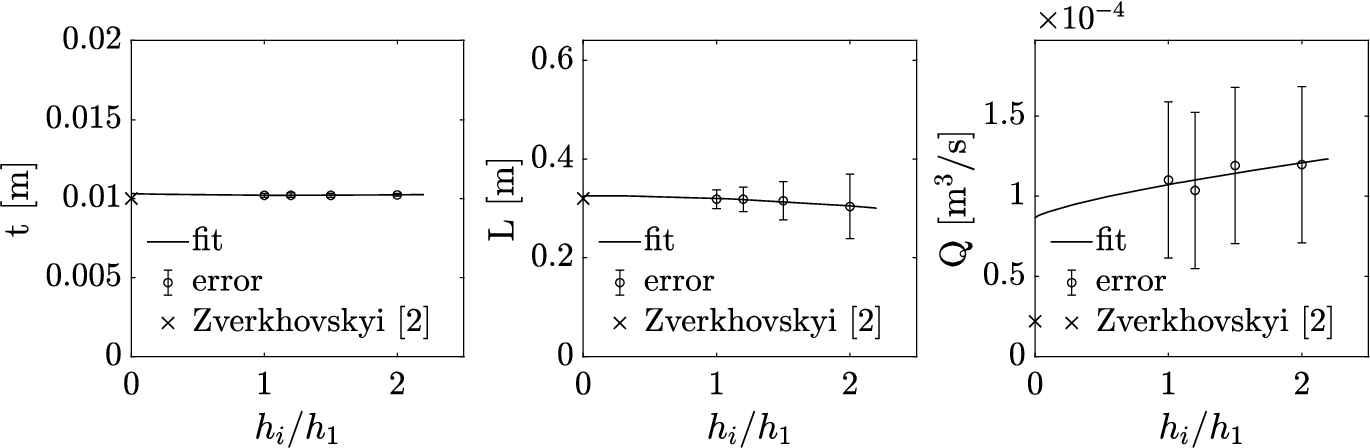
For the cavity thickness, the estimated discretization uncertainty lies between 0.9–1.4%. For the cavity length it is between 5.9–21%, which is also reasonably small for the finer grids. However, for the air flow rate it is 44.2%. Figure 8 shows the spatial discretization uncertainty fits for the cavity thickness, length and air flow rate. The error bars indicate the uncertainties of their specific data points.
Fig. 8.
Spatial discretization uncertainty fits for the mean cavity thickness, cavity length and required air flow rate. The convergence orders for the fits (p) are stated in Table 3.
3.2.Cavity profiles and required air flow rate
For all simulations, the computed time-averaged length and thickness are in very good agreement with the expected cavity length L of 0.32 m and thickness t of 0.01 m following from linear wave theory and the experiments from Zverkhovskyi [2]. The time-averaged results for the finest grid are given in Table 4. However, the cavity profiles as computed on all grids with all time steps did not show correct cavity closure behaviour. An example of the time-averaged cavity profile is shown in Fig. 9. A thin layer of air is constantly present in the closure region (around
Table 4
Time-averaged cavity length, thickness and required air flow as computed on the finest grid with
| Simulation | Experiment | |
| 0.01 | 0.01 | |
| 0.32 | 0.32 | |
Fig. 9.
Time-averaged cavity profile as computed on the finest grid with
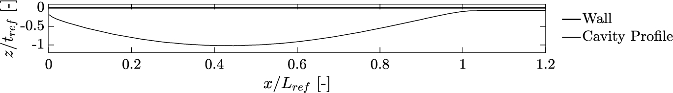
Fig. 10.
Pressure distribution and velocity field in the closure area of the air cavity. The contour lines indicate the air volume fraction α from 0.5 to 0.98. Flow from left to right.
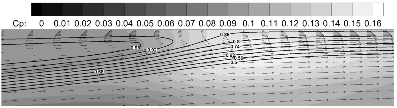
Fig. 11.
The computed ensemble-averaged boundary layer profiles at three different stream-wise locations: from left to right; upstream, in the middle and downstream of the cavity (from case
![The computed ensemble-averaged boundary layer profiles at three different stream-wise locations: from left to right; upstream, in the middle and downstream of the cavity (from case hi/h1=2 and ti/t1=1). The simulations from the current project are compared to the time-averaged experimental data from Zverkhovskyi [2].](https://ip.ios.semcs.net:443/media/isp/2019/66-4/isp-66-4-isp190270/isp-66-isp190270-g011.jpg)
3.3.Boundary layer profiles around the air cavity
The boundary layers as computed were compared to the experimental data from Zverkhovskyi [2]. Figure 11 shows the computed ensemble-averaged velocity profiles in the boundary layer 3 cm upstream, in the middle, and 3 cm downstream of the air cavity and the profiles compare well with the measured time-averaged profiles. The computed upstream profile slightly differs from the experimental one, since there is a small under-prediction of the velocity between 0.25 and 0.8
Unfortunately, the results of the experimental measurements close to the wall are of insufficient resolution to quantitatively compare the viscous sub-layer of the boundary layer, which determines the wall shear stress. Moreover, due to the constant presence of the thin layer of air downstream of the cavity in all simulations (Fig. 9), the wall shear stress was not correctly computed downstream of the cavity and no results can be presented with regard to the overall friction drag.
3.4.Eddy-viscosity correction
Figure 12 shows the computed cavity profiles for a case without eddy-viscosity correction and one case with the power correction function as proposed by Reboud et al. [23] and Coutier-Delgosha et al. [25]. The profile as computed with the activated correction based on the power function is very unstable. The instability of the cavity interface (Fig. 12) is present for a range of power values
Fig. 12.
Cavity profiles for the case without eddy-viscosity correction and for the eddy-viscosity correction case where the power function was applied. Flow from left to right.
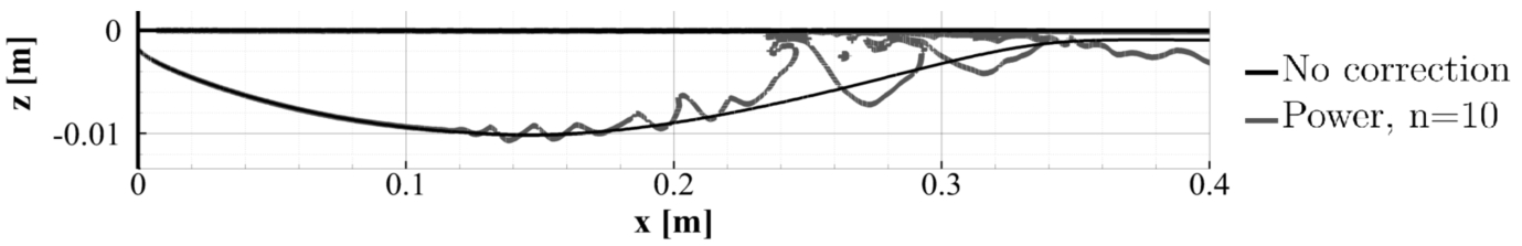
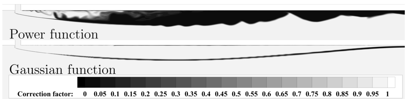
Fig. 13.
Regions where the eddy-viscosity correction function was active. Top: power function. Bottom: Gaussian function. 1: no reduction of produced eddy-viscosity, 0: maximum reduction of produced eddy-viscosity. Flow from left to right.
The Gaussian correction function was applied with
4.Discussion
4.1.Cavity profiles and boundary layer profiles
With the set pressure at the air inlet, the global cavity profile as computed on all grids was in good agreement with the experimental profile from Zverkhovskyi [2] as well as with linear theory. However, the spatial discretization uncertainty for the cavity length (5.7% for the finest grid and around 20% for the coarsest grid) is a bit higher when compared to the spatial discretization uncertainty for the cavity thickness (maximum of 1.4% on all grids). That the cavity length is more sensitive to the local grid size can be explained by the chosen grid topology as well as from the observation that the solution is more diffuse in the direction of the flow.
Whilst the cavity profile should not be dependent on the prescribed pressure, the cavity length, as well as the thickness, increased while increasing the pressure difference (Fig. 4). The experimental data shows a stable cavity profile, which incidentally leaks small pockets of air. In the simulations, however, a thin layer of air/water mixture is continuously present at the closure and downstream of the cavity, resulting in an under-estimation of the computed wall shear stress. The ensemble-averaged velocity profiles in the boundary layer upstream and the middle of the air cavity compare well with the measured time-averaged profiles. Only the computed velocity profile downstream of the cavity shows an overestimation of the velocity close to the wall, most probably due to the smeared air-water interface present here.
4.2.Closure behaviour and required air flow rate
This study aimed to model a re-entrant jet in the closure of an external air cavity. In analogy with the modelling of vaporous sheet cavities, two different eddy-viscosity correction functions were applied to the problem. However, the computed results did not show a re-entrant jet in the closure region of the cavity. This implies that solely correcting the eddy-viscosity on the air-water interface is insufficient to initiate air leakage by re-entrant jet. However, the computed eddy-viscosity at the cavity interface as well as inside the cavity has a large influence on the interface stability, as shown in Fig. 12. The present eddy-viscosity provides additional stiffness for the cavity interface, but it is not sufficient to only reduce the eddy-viscosity around the interface. The solution of the cavity interface becomes very unstable for large eddy-viscosity reductions, as shown for the power function.
Most probably, the asymmetric nature of the power function (as shown in Fig. 6) reducing almost all eddy-viscosity in the gas phase, is the reason for the cavity profile instability. Due to the instabilities on the cavity interface, the iterative convergence stagnates an order of magnitude higher compared to the default turbulence model. The air volume fraction inside the cavity is equal to or larger than 0.99. However, due to the bias of the power correction function towards the low-density fluid, all eddy-viscosity inside the cavity is reduced such that there is no eddy-viscosity at all. The total viscosity difference between inside and outside the cavity is approximately ten times lower for the power correction cases compared to the default cases. Next to this difference, the total eddy-viscosity outside the cavity is rather high, due to the developed boundary layer upstream of the cavity (
However, whilst the Gaussian correction function only applies the correction at the cavity interface, it resulted in more or less the same time-averaged cavity profile as found for the standard turbulence model simulations. Consequently, in all cases, also including an ad-hoc eddy-viscosity correction function, no shedding of air pockets or re-entrant jet was observed. This raises two questions. Either it is questionable whether or not the re-entrant jet should be there for these cases, or this RANS-VoF approach is not capable of simulating it.
Initially, an analogy was assumed with vapour cavitation. Both in the physical description of the re-entrant jet behaviour, as well as in the numerical modelling of the problem. Regarding the physical description of the flow, there are two main differences. Firstly, the pressure gradient at the cavity closure is weak for air cavities, whereas it is moderate to strong for vapour cavities. The question then arises whether this pressure difference is high enough to create a re-entrant jet for this air cavity case. The pressure distribution in Fig. 10 shows that there is a region with higher pressure in the cavity closure, but the pressure gradient is relatively weak. However, the velocity field shows a region with reversed flow in the closure area, and with a mixture flow. One could argue this is a re-entering flow. Secondly, the air cavity is formed within a developed boundary layer, which potentially hampers the formation of the re-entering flow due to the lower local velocities.
Next to the differences in the physical description of the flow, there are several differences regarding the modelling of the air cavity problem compared to the vapour sheet cavity problem. Firstly, for the air cavity problem, there is no cavitation model active in the simulations, so there are no source/sink terms active to produce and destroy the air phase as they are in vapour cavitation modelling. Nevertheless, solely complementing the RANS equation with a cavitation model is not enough to model the re-entrant jet shedding behaviour either, as shown by e.g., Coutier-Delgosha et al. [25]. However, this study shows that solely correcting the eddy-viscosity in the interface region, on the other hand, is also not enough to model the re-entrant jet.
Thirdly, as follows from the physical difference described above, the developed boundary layer in which the air cavity is formed results in a high eddy-viscosity ratio around the air interface, which possibly hampers the formation of the re-entrant jet.
Additionally, the RANS modelling of natural cavitation problems usually asks for a low-order and thus diffuse discretization scheme for the volume fraction equation. Here a higher-order compressive scheme is used, since in the current approach the stable cavity interface till the closure should be solved as well, especially when one is also interested in the wave pinch-off mechanism and the total air flux leaving the cavity.
The contour plot of the air volume fraction, as given in Fig. 10, shows a thick smeared interface in the closure region. Even though compressive schemes are used, this indicates a numerical artefact that often occurs with single-fluid VoF methods, if the interface contains curvatures or is not parallel with the grid cell faces. Theoretically, the transport equation for the air volume fraction should not result in such a diffuse interface for a pure advection problem. However, due to discretization errors, iterative errors, and the use of TVD limiters, the solution will always show some numerical diffusion [30]. The smeared interface possibly results in momentum-loss of the re-entering flow.
A possible solution, but currently not available, could be switching to higher-order discretization schemes. Also, grid refinement could sharpen the interface and should eventually decrease the discretization uncertainty for the air flow rate. Shiri et al. imply this as well [8]. However, this also implies grid refinement upstream, along the complete cavity profile, to avoid numerical diffusion as much as possible. While the computed spatial discretization uncertainty seems very large, it should be mentioned that the air flow rate itself is small, i.e., in the order of litres per minute, and only is due to the smeared air-water interface near the flat plate. Therefore the order of convergence p is not second-order, but from an engineering point of view, the current uncertainties seem to be exaggerated.
Another methodology approach could also be studied, e.g., geometrical reconstruction of the interface like VoF-PLIC, a Eulerian multiphase model that solves the momentum and continuity equations for each phase or a (coupled) Level-Set VoF approach.
5.Conclusions and further work
The simulated velocity profiles at different stream-wise locations in the boundary layer around the cavity compare well to the experimental profiles. However, the mismatch which was found in the determination of the cavity profile and required air flow rate for the cavity is hypothesized to follow from the incorrect flow modelling with a bias to the VoF method based on a single-fluid formulation for free surface modelling in the closure region. Solving the closure probably requires a different approach for modelling the multiphase flow, e.g., solving the momentum equations for each fluid, a VoF-PLIC, or a Level-Set approach.
It is questionable whether the re-entrant jet is indeed the main shedding mechanism for air cavities. Also after including an ad-hoc eddy-viscosity correction model, no shedding mechanism was observed. The presence of eddy-viscosity at the cavity interface as well as inside the cavity and upstream of the cavity have a large influence on the interface stability, and the exact mechanism for air discharge at the cavity closure is still not clear.
Other turbulence models such as a Reynolds Stress Model could improve the turbulent behaviour of the flow in front and along the cavity, since the isotropic turbulence modelling as used in classical linear eddy-viscosity models is a violation of the anisotropic nature of the turbulence structures near the interface.
Next to the modelling of the re-entrant jet, the wave pinch-off mechanism also needs to be modelled in order to capture the cavity closure mechanisms. Since wave pinch-off is hypothesized to be governed by waves formed by turbulence structures hitting the interface, it is known a-priori that this mechanism can not be simulated directly with a RANS solver. A scale-resolving or hybrid model such as LES, RANS-LES or PANS would then be required.
Therefore, future work focuses on the use and capabilities of scale resolving simulations to study the physical conditions in front of and along the cavity, such as the influence of turbulence on the behaviour of the cavity interface.
Acknowledgements
We thank the Dutch Research Council (NWO), by whom this work is financially supported as part of the ShipDRAC project (13265). The work was carried out on the Reynolds (TU Delft) and Marclus3 (MARIN) clusters.
References
[1] | Y. Gorbachev and E. Amromin, Ship drag reduction by hull ventilation from laval to near future: Challenges and successes, in: Association Technique Maritime et Aeronautique, (2012) . |
[2] | O. Zverkhovskyi, Ship drag reduction by air cavities, PhD thesis, Delft University of Technology, 2014. |
[3] | S.A. Mäkiharju, The dynamics of ventilated partial cavities over a wide range of Reynolds numbers ans quantitative 2D X-Ray densitometry for multiphase flow, PhD thesis, The University of Michigan, 2012. |
[4] | A.A. Butuzov, Limiting parameters of an artificial cavity formed on the lower surface of a horizontal wall, Fluid Dynamics 1: (2) ((1966) ), 116–118. doi:10.1007/BF01013836. |
[5] | K.I. Matveev, On the limiting parameters of artificial cavitation, Ocean Engineering 30: ((2003) ), 1179–1190. doi:10.1016/S0029-8018(02)00103-8. |
[6] | S.L. Ceccio, Friction drag reduction of external flows with bubble and gas injection, Annual Review of Fluid Mechanics 42: ((2010) ), 183–203. doi:10.1146/annurev-fluid-121108-145504. |
[7] | S. Mäkiharju, B. Elbing, A. Wiggins, S. Schinasi, J.-M. Vanden-Broeck, M. Perlin and D.R. Dowling, On the scaling of air entrainment from a ventilated partial cavity, Journal of Fluid Mechanics 732: ((2013) ), 47–76. doi:10.1017/jfm.2013.387. |
[8] | A. Shiri, M. Leer-Andersen, R.E. Bensow and J. Norrby, Hydrodynamics of a displacement air cavity ship, in: 29th Symposium on Naval Hydrodynamics, (2012) . |
[9] | L. Barbaca, B. Pearce and P.A. Brandner, Experimental study of ventilated cavity flow over a 3-D wall-mounted fence, International Journal of Multiphase Flow 97: ((2017) ), 10–22. doi:10.1016/j.ijmultiphaseflow.2017.07.015. |
[10] | L. Barbaca, B. Pearce and P.A. Brandner, An experimental study of cavity flow over a 2-D wall-mounted fence in a variable boundary layer, International Journal of Multiphase Flow 105: ((2018) ), 234–249. doi:10.1016/j.ijmultiphaseflow.2018.04.011. |
[11] | M. Callenaere, J. Franc, J. Michel and M. Riondet, The cavitation instability induced by the development of a re-entrant jet, Journal of Fluid Mechanics 444: ((2001) ), 223–256. doi:10.1017/S0022112001005420. |
[12] | S. Menon, R. Bensow and C. Eskilsson, Investigation of numerical schemes in air cavity computations, in: International Conference on Hydrodynamics, Egmond Aan Zee, The Netherlands, (2016) . |
[13] | O. Zverkhovskyi, M. Kerkvliet, A. Lampe, G. Vaz and T. van Terwisga, Numerical study on air cavity flows, in: 18th Numerical Towing Tank Symposium (NuTTS), Cortona, Italy, (2015) . |
[14] | D. Kim and P. Moin, Direct numerical simulation of air layer drag reduction over a backward-facing step, Center for Turbulence Research Annual Research Briefs (2010), 351–363. |
[15] | G. Rotte, F. Charruault, M. Kerkvliet and T. van Terwisga, An investigation on the set-up of air cavity simulations using a scale resolving method, in: 21st Numerical Towing Tank Symposium (NuTTS), Cortona, Italy, (2018) . |
[16] | G. Rotte, F. Charruault, M. Kerkvliet and T. van Terwisga, On the limitations and capabilities of LES for air cavity flows, in: 10th International Conference on Multiphase Flow (ICMF), Rio de Janeiro, Brazil, (2019) . |
[17] | G. Rotte, O. Zverkhovskyi, M. Kerkvliet and T. van Terwisga, On the physical mechanisms for the numerical modelling of flows around air lubricated ships, in: International Conference on Hydrodynamics (ICMF), (2016) . |
[18] | G. Rotte, M. Kerkvliet and T. van Terwisga, On the turbulence modelling for an air cavity interface, in: 20th Numerical Towing Tank Symposium (NuTTS), Wageningen, The Netherlands, (2017) . |
[19] | G. Rotte, M. Kerkvliet and T. van Terwisga, On the influence of eddy viscosity in the numerical modelling of air cavities, in: The 10th International Conference on Cavitation (CAV2018), Baltimore, Maryland, USA, (2018) . |
[20] | MARIN, ReFRESCO, 2019, [Online; http://www.refresco.org, accessed 8-11-2019]. |
[21] | F. Menter, Y. Egorov and D. Rusch, Steady and unsteady flow modelling using the |
[22] | P. Roe, Characteristic-based schemes for the Euler equations, Annual Review of Fluid Mechanics 18: ((2003) ), 337–365. doi:10.1146/annurev.fl.18.010186.002005. |
[23] | J. Reboud, B. Stutz and O. Coutier, Two-phase flow structure of cavitation: Experiment and modelling of unsteady effects, in: 3rd International Symposium on Cavitation, (1998) . |
[24] | I.A. Hannoun, H.J.S. Fernando and E.J. List, Turbulence structure near a sharp density interface, Journal of Fluid Mechanics 189: ((1988) ), 189–201. doi:10.1017/S0022112088000965. |
[25] | O. Coutier-Delgosha, R. Fortes-Patella and J. Reboud, Evaluation of the turbulence model influence on the numerical simulations of unsteady cavitation, Journal of Fluids Engineering 125: (1) ((2003) ), 38–45. doi:10.1115/1.1524584. |
[26] | L. Eça and M. Hoekstra, On the influence of the iterative error in the numerical uncertainty of ship viscous flow calculations, in: 26th Symposium on Naval Hydrodynamics 2006, (2006) , pp. 17–22. |
[27] | L. Eça and M. Hoekstra, A procedure for the estimation of the numerical uncertainty of CFD calculations based on grid refinement studies, Journal of Computational Physics 262: ((2014) ), 104–130. doi:10.1016/j.jcp.2014.01.006. |
[28] | G.F. Rosetti, G. Vaz and A.L.C. Fujarra, URANS calculations for smooth circular cylinder flow in a wide range of Reynolds numbers: Solution verification and validation, in: Proceedings of the International Conference on Offshore Mechanics and Arctic Engineering – OMAE, (2012) . doi:10.1115/OMAE2012-83155. |
[29] | J. Brouwer, J. Tukker and M. van Rijsbergen, Uncertainty analysis and stationarity test of finite length time series signals, in: 4th International Conference on Advanced Model Measurement Technology for the Maritime Industry (AMT15), Istanbul, Turkey, (2015) . |
[30] | M.S. Darwish and F. Moukalled, TVD schemes for unstructured grids, International Journal of Heat and Mass Transfer 46: (4) ((2003) ), 599–611. doi:10.1016/S0017-9310(02)00330-7. |


