
Financial sentiment analysis: Classic methods vs. deep learning models
Abstract
Sentiment Analysis, also known as Opinion Mining, gained prominence in the early 2000s alongside the emergence of internet forums, blogs, and social media platforms. Researchers and businesses recognized the imperative to automate the extraction of valuable insights from the vast pool of textual data generated online. Its utility in the business domain is undeniable, offering actionable insights into customer opinions and attitudes, empowering data-driven decisions that enhance products, services, and customer satisfaction. The expansion of Sentiment Analysis into the financial sector came as a direct consequence, prompting the adaptation of powerful Natural Language Processing models to these contexts. In this study, we rigorously test numerous classical Machine Learning classification algorithms and ensembles against five contemporary Deep Learning Pre-Trained models, like BERT, RoBERTa, and three variants of FinBERT. However, its aim extends beyond evaluating the performance of modern methods, especially those designed for financial tasks, to a comparison of them with classical ones. We also explore how different text representation and data augmentation techniques impact classification outcomes when classical methods are employed. The study yields a wealth of intriguing results, which are thoroughly discussed.
1.Introduction
The computational study of people’s sentiments, opinions, assessments, attitudes, and emotions regarding entities and their characteristics expressed in text is commonly referred in the literature as Sentiment Analysis (SA) or Opinion Mining (OM) [1]. This scientific field is considered to be a subdomain of Natural Language Processing (NLP) and experienced a significant development following the advent of Web 2.0. In our contemporary times, more than ever before, a substantial portion of human activities unfolds in the online realm. Businesses and services have swiftly adjusted to the digital landscape, presenting online platforms for a spectrum of activities, including shopping, banking, communication, entertainment, and beyond. This phenomenon, widely recognized as digital transformation, is indeed a hallmark of our era. Furthermore, online work and learning offer a remarkable degree of flexibility and convenience, a reality that became especially evident during the COVID-19 pandemic. Social media platforms enable individuals to connect, engage, share information, and exchange viewpoints. Simultaneously, streaming and on-demand services have captured a significant segment of the entertainment market. The substantial volume of online activities has resulted in the generation of a vast amount of data containing valuable information that holds the potential to benefit numerous areas of human activity.
In specific domains such as industry, markets, and digital entertainment, the viewpoints of customers or service users play a pivotal role. This significance arises not only from gathering feedback but also from enhancing the quality of services and fostering the growth of products. This is when the need for systematic extraction of meaningful information from user product reviews [2], films and movies [3, 4] emerged. The engagement of users on social networks, coupled with their activities within these platforms, constitutes an immense wellspring of information. This resource can be effectively harnessed to extract insights into the opinions and intentions of individuals a task that, prior to the internet’s expansion, would have required substantial effort, time, and financial investment. The necessity for extracting insights from user comments on social media platforms such as Facebook [5], YouTube [6], and Twitter [7, 8, 9] also led to the advancement of methodologies and tools for SA. For a contemporary comprehensive overview of SA in the aforementioned social media domains, the interested reader is referred to [10].
Besides social media – but in some cases through social media posts – SA found applications in domains such as healthcare [11, 12, 13, 14], politics [15, 16, 17], public policy [18], psychology [19, 20], marketing [21], scientific citations [22] business [23, 24, 25] and finance [26] and so on. In [27], the authors formulated a taxonomy of research topics in which the interested reader can seek additional information on SA application domains.
Financial Sentiment Analysis (FSA) can be defined as the application of concepts and methods of SA in the financial domain and, more specifically, in documents of financial nature. FSA can be a valuable tool for traders, investors, financial institutions, and analysts to gauge market sentiment, assess risks, and make more informed financial decisions. The underlying philosophy for the uprise of SA in the financial domain is that the Efficient Market Hypothesis (EMH) seems to give its position to the Adaptive Market Hypothesis (AMH) due to criticism from behavioural economics [26]. According to EMH theory, financial markets are perfectly efficient and asset prices always reflect all available information. The AMH challenges the strict assumptions of EMH. It acknowledges that market participants are not always perfectly rational and that market dynamics can change over time. AMH suggests that market participants adapt to new information and market conditions, and this adaptation can lead to changes in asset prices. In a dynamic and ever-evolving environment, the active processing and assessment of every incoming piece of information are deemed vital for shaping future decisions. Consequently, the significance of employing SA techniques in matters pertaining to financial data can be exceptionally advantageous and profitable, guiding stakeholders towards more informed choices and decisions. Examples where SA is applied in the financial world are abundant. Stock prediction [28], FOREX exchange rate prediction [29], market volatility [30], asset allocation [31, 32], credit worthiness [33], initial public offering valuation (IPO) [34], cryptocurrency [35, 36, 37, 38] are – among numerous others – some applications of SA in financial domain.
It is essential to recognize that FSA comes with unique challenges. Factors such as the limited availability of extensive data and the complexity of annotating financial texts without domain expertise or expert input [39] set it apart from SA in more general contexts. For instance, financial documents like reports, social media posts, and news articles are replete with specialized terminology, economic jargon, and technical terms. Any inaccuracies in FSA can have severe and unacceptable consequences, potentially leading to significant financial losses. As a result, findings derived from FSA demand careful evaluation and should be approached with a high degree of caution. In the financial domain, where decisions can have far-reaching impacts on investments and markets, the necessity for precision in sentiment analysis cannot be overstated. Rigorous methodologies, access to accurate domain-specific data, and collaboration with experts in the field are indispensable in ensuring the reliability of FSA outcomes.
The conventional SA techniques may not exhibit the same level of effectiveness within the financial domain. The performance of existing models tends to degrade when applied to FSA as opposed to more traditional SA tasks. This underscores the importance of critically assessing and adapting the existing methodologies to suit the unique demands of the economic domain. The process of evaluation serves as a compass to help us identify and embrace the most efficacious techniques for FSA. Meanwhile, modification efforts pave the way for developing more tailored and efficient methodologies suited explicitly to this intricate domain. In essence, through evaluation and modification, we can enhance the applicability and precision of SA within finance.
The structure of this study is as follows: In Section 2, we conduct a comprehensive review of recent literature pertaining to the current research. In Section 3, we provide detailed insights into the experimental setup, including the dataset employed, the pre-processing methodology, the ML models utilized, and the metrics for evaluating model performance. Section 4 presents the outcomes of the aforementioned experimental process. Finally, the paper is concluded in the Conclusions section.
2.Literature review
Three primary approacheslexicon-based, machine learning, and hybridconstitute the main methodologies employed for SA in the general domain, as highlighted in [40]. In the context of financial SA, these three methodologies remain pivotal, each with its own unique characteristics. Lexicon-based methods, for instance, diverge into two categories: generic lexicon-based methods, as discussed in [41], and domain-specific lexicon-based methods, like those tailored for the financial sector. The initial group of methods, characterized by a significant misclassification rate, has since given way to the adoption of financial lexicon-based methods. This shift was pioneered by Loughran and McDonald in their work [42], marking the inception of financial lexicon development. Subsequently, research in this domain has continued unabated, exemplified by recent contributions such as the ones presented in [43, 44, 45].
Sometimes, it is difficult to distinguish which approach a paper uses because many of them use a mix of methods. For instance, the LPS model [46] is a widely cited example in recent research papers. It’s used as a basic model to predict the meaning of words in short economic texts, especially in finance. The model works by understanding finance-specific terms and their meanings in three stages: in the first two stages, it uses sentence structure and domain knowledge, and in the final stage, it uses a special type of classifier. This approach is in line with the current trend in research where traditional ML and deep learning models are combined with methods that select important words from lexicons and process sentences or individual words, as discussed in [47]. Although some researchers, like those in [40], distinguish between ML and Neural Network approaches, we consider it part of the broader ML category for our study. Since our focus is mainly on ML, this literature review concentrates on methods within that domain. FinSSLx [48] is a multi-class classifier for financial sentiment analysis using a layer for simplifying text based on phrases or clauses followed by a LSTM neural network. This model seems to outperform the LPS and Reduced-LPS models [46].
When considering the deployment of classical ML models in FSA scenarios, a multitude of studies can be found in recent literature. For instance, in [49], the authors employ a Support Vector Machine (SVM) approach optimized through particle swarm optimization (PSO) for SA stock market prediction. Similarly, [50] employs Multivariate Linear Regression in conjunction with SA techniques to address the same stock market prediction problem. In [51], seven well-established ML algorithms are applied, leveraging SA on data sourced from microblogging sites to predict stock prices. SVMs are also employed in [28] in tandem with SA to forecast stock market movement directions. In [52], three prominent ML algorithmsNeural Networks (NN), SVMs, and Random Forest (RF) are compared for predicting cryptocurrency market movements. They utilize pertinent information from Twitter and market data as input features. Lastly, regarding studies where a wide array of classical ML methods are compared in financial domain tasks, along with the incorporation of SA, [53] employs twenty-seven ML models on a comprehensive dataset. This extensive analysis encompasses various sentiment configurations to predict the closing prices of fifteen companies in the financial markets.
It was evident that the emergence of Deep Learning models would significantly impact the field of FSA. These more advanced models started to find application in financial tasks, yielding impressive results. In [54], a range of neural network models, including Long Short-Term Memory (LSTM), Doc2Vec, and Convolutional Neural Networks (CNNs), were employed to analyze stock market opinions extracted from StockTwits. The goal was to predict the sentiment of the authors. Furthermore, [55] delved into the utilization of traditional LSTM and attention-based LSTM deep neural networks for predicting future stock market movements, incorporating SA on data collected from Twitter. In [56], various deep learning architectures, spanning from Multilayer Perceptrons (MLPs) to CNNs and Recurrent Neural Networks (RNNs), were harnessed alongside sentiment data gathered from diverse online sources to detect changes in Bitcoin prices. Regarding the real-time BITCOIN price prediction, [57] leveraged RNNs equipped with LSTMs in conjunction with data extracted from Twitter and Reddit. [58] presented an extensive comparative study encompassing thirty contemporary Deep Learning models, with the aim of not only shedding light on model performance but also exploring a multitude of sentiment feature configurations. For a more comprehensive understanding of the application of modern Deep Learning methods in the FSA domain, additional information can be found in the following survey papers: [59, 60, 61].
After the emergence of general language representation models like BERT and RoBERTa (further information on these models can be found in next session), domain-specific models based on the pre-existing general ones began to appear. FinEAS model [62], for example, is based on the Sentence-BERT model with an extra linear layer for regression due to the reason that sentiment is modelled as a continuous variable (
At this point, it should be noted that in this section, only a representative portion of the relevant literature is provided. The reader is encouraged to use these sources as a starting point for further in-depth research.
3.Experimental procedure
3.1Dataset description
The publicly available financial dataset [69] was used for the experimental procedure. This dataset resulted from the merging of two separate datasets FiQA [70] and Financial PhraseBank [71] combined into a ready to use csv file.
The FiQA dataset, introduced for the WWW ’18 conference’s financial OM and question-answering competition [70], comprises questions and answers rooted in financial reports. This dataset has gained significant prominence as it serves as a valuable resource for training and assessing NLP models, particularly those tailored for finance-related tasks. Notably, FiQA provides sentiment scores ranging continuously from
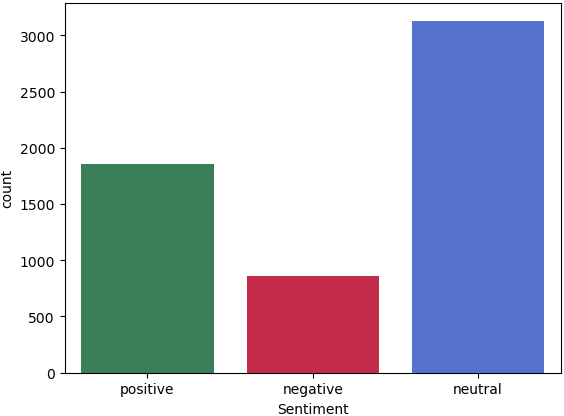
The resultant dataset comprises 5,842 labelled financial sentences, categorized as positive (1), neutral (0), or negative (
Another noteworthy concern pertains to the potential presence of similar sentences assigned different sentiment labels. For instance, consider the following sentences: “Earnings per share (EPS) amounted to a loss of EUR0.05” and “Earnings per share (EPS) amounted to a loss of EUR0.06.” These sentences exhibit close semantic meaning and, according to the authors, should ideally carry the same sentiment score. However, it remains unclear how many sentences fall into this category, warranting further investigation. The implication of the above issue may be the reduced performance of any algorithm we use for SA in sequel.
In Fig. 1, the distribution of sentences in the dataset among the three classes is presented. It is observed that the number of sentences falling into each class is not evenly distributed. The count of sentences labelled as neutral is significantly higher than that of the other classes, while those labelled as negative constitute the smallest percentage of the dataset. As a result, this specific dataset can be considered as an imbalanced one.
Figure 1.
Distribution of instances among classes.
3.2Pre-processing procedure
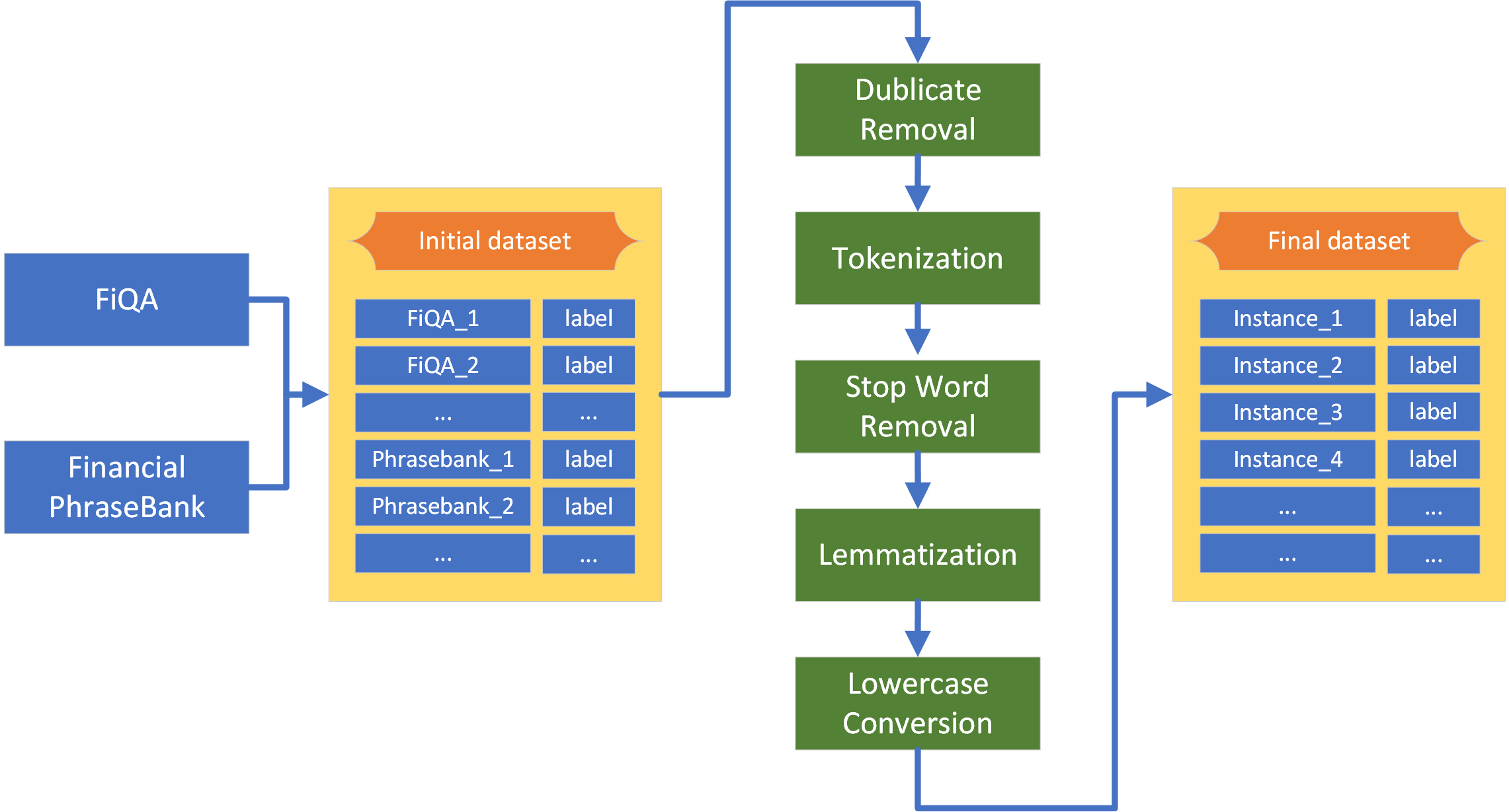
The next step after creating the dataset is its pre-processing. Data pre-processing is a significant phase of the experimental process in SA scenarios, allowing the data to acquire the appropriate structure for subsequent use by ML algorithms. The steps that were followed are presented below, both in natural language and graphically, as depicted in Fig. 2, to provide the reader with a clearer understanding of the process.
Concerning the above, data pre-processing includes the following steps:
• Duplicate Removal: We identified approximately 520 duplicated sentences with potentially different sentiments. As a prepossessing step, we opted to remove these duplicates.
• Tokenization: Tokenization is a fundamental technique in NLP that dissects text strings into sequences of words (tokens) [73]. For this purpose, we utilized the Python NLTK library in this study.
• Stop Word Removal: Although not universally applicable, removing of stop words is a common practice in text prepossessing. This is done to prioritize meaningful words and reduce the overall number of tokens (words) [73].
• Lemmatization: In this study, we chose lemmatization over stemming. While both techniques aim to normalize text, lemmatization tends to deliver better performance with minimal computational overhead [73]. We employed the WordNet Lemmatizer package available in the Python Natural Language Toolkit (NLTK).
• Lowercase Conversion: Lowercasing is a standard text normalization technique, as word meanings remain consistent regardless of letter case. Research has shown that converting text to lowercase can enhance SA performance [74].
Figure 2.
Pre-processing stage.
3.3Machine learning models
In the context of this work, a plethora of algorithms was utilized, which can be categorized into two groups: the first group comprises classical ML algorithms for classification problems, as well as ensembles of some of them. The second group pertains to a series of Deep Learning Pre-trained Models, which represent a more promising approach for tackling NLP problems. Subsequently, the necessary information about the models used is provided to describe the outline of the experimental process.
In this study, classical ML models were trained and evaluated using the PyCaret [75] library. PyCaret is a powerful open-source low-code ML toolkit written in Python, functioning as a versatile wrapper for various Python libraries, including scikit-learn. It streamlines the ML pipeline, enabling practitioners to efficiently train and test a range of algorithms for both supervised (e.g., classification) and unsupervised learning tasks with just a few lines of code. The complete list of models used, along with their abbreviations can be found in Table 1.
Table 1
List of classic ML classification algorithms
| Method | Abbreviation | |
|---|---|---|
| 1 | AdaBoost Classifier | AdaBoost |
| 2 | CatBoost Classifier | CatBoost |
| 3 | Decision Tree Classifier | DT |
| 4 | Dummy Classifier | DC |
| 5 | Extra Trees Classifier | ET |
| 6 | Extreme Gradient Boosting | XGBoost |
| 7 | Gradient Boosting Classifier | GBC |
| 8 | K-Nearest Neighbors | KNN |
| 9 | Light Gradient Boosting Machine | LightGBM |
| 10 | Linear Discriminant Analysis | LDA |
| 11 | Logistic Regression | LR |
| 12 | Naive Bayes | NB |
| 13 | Quadratic Discriminant Analysi | QDA |
| 14 | Random Forest Classifier | RF |
| 15 | Ridge Classifier | Ridge |
| 16 | Support Vector Machine | SVM |
Note that the Dummy Classifier used in this context is a Stratified Dummy Classifier, which predicts class labels in a manner that mirrors their distribution in the training dataset. This strategic choice ensures that the baseline model generates predictions that accurately reflect the natural class distribution in the data. By doing so, it establishes a meaningful starting point for the comparison and evaluation of other ML models. An extra pre-processing technique that we use for testing classical ML models is Bag of Words (BoW), which is implemented in Pycaret. Alternatively, it can be used Term Frequency – Inverse Document Frequency (TF-IDF) weighting using PyCaret ecosystem.
The Bag of Words (BoW) approach constructs a vector for ML models by tallying the occurrences of each unique word in the corpus. To create a BoW representation, a vocabulary is initially compiled from all unique words in a collection of documents. Each document is then depicted as a vector, with each vector dimension corresponding to a word in the vocabulary. The value in each dimension signifies how many times that word appears in the document. This results in a sparse numerical representation of text data, where each document essentially represents a count of word occurrences. The TF-IDF approach is considered to be the product of two distinct statistical measures: TF (Term Frequency) and IDF (Inverse Document Frequency). The TF measure quantifies the number of times a term occurs within the entire document, reflecting the importance of the word within that specific document. Meanwhile, the IDF measure gauges the rarity of each term across the entire document corpus and is calculated by taking the logarithm of the total number of documents in the corpus divided by the number of documents containing the word. Finally, the TF-IDF score for a word in a document is calculated by multiplying its TF and IDF values. This results in a numerical representation where each document is characterized by the TF-IDF scores of its words. Higher TF-IDF scores signify that a word is significant within a particular document but relatively infrequent across the entire corpus.
Both techniques come with their own set of advantages and disadvantages. BoW is straightforward and easy to understand, involving basic counting operations, which makes it computationally efficient even when dealing with large text corpora. However, BoW does not capture word semantics or relationships between words, making it less suitable for tasks that require understanding meaning. On the other hand, TF-IDF considers the importance of words within individual documents and the entire corpus, capturing the context and significance of words. It scales well to large text corpora and remains effective even with extensive datasets. However, its calculation can be more computationally intensive compared to BoW, especially with such datasets. It is worth noting that both techniques have the drawback of ignoring word order in sentences, leading to a loss of context and potentially important information. Although in detecting hate speech [76] TF-IDF performed better than Bow for the same classifiers, in the present paper, we will use both as an attempt to compare them in FSA.
As referenced in Section 3.1, the dataset used in this study exhibits class imbalance. To address this issue, we employ two approaches. In the first approach, we utilize both stratified k-fold cross-validation and Synthetic Minority Over-sampling Technique (SMOTE). SMOTE is an ML method designed to mitigate class imbalance by generating artificial data points for the minority class, resembling existing instances through a process of selecting each minority class example and identifying its nearest neighbors, creating new synthetic instances as interpolations between them. By incorporating these synthetic examples into the dataset, SMOTE enhances the learning process of ML models, making them more effective at handling imbalanced data and improving overall predictive accuracy. Notably, SMOTE has been applied successfully in SA, resulting in improved classifier performance [77, 78]. In the second approach, we rely solely on Stratified k-fold cross-validation. These approaches enable us to compare whether the inclusion of SMOTE leads to superior classification results for each classifier.
A classic method to enhance classification accuracy involves building a meta-ensemble ML model that combines the top-performing models, typically three in number, as measured by the Matthews Correlation Coefficient (MCC). MCC is considered a superior metric to F1 score and accuracy, particularly in datasets with imbalanced classes [79]. Two primary approaches are commonly used to aggregate classifier results: hard voting and soft voting.
The hard voting technique, also known as majority voting, entails each individual classifier casting a vote for a class, and the class with the most votes becomes the final prediction. Conversely, soft voting involves calculating the average probabilities for each class across the individual classifiers, and the class with the highest average probability is chosen as the final prediction. Both of these techniques are not unfamiliar in the domain of SA. For instance, in [80], soft voting is employed to formulate a meta-ensemble classifier for SA in movie reviews, while in [81] hard voting is utilised for sentiment analysis on Twitter data related to airline services. In our research, we opt for the soft voting technique due to its consideration of confidence levels, making it a more sophisticated and suitable choice.
As a result of the above we are going to run using PyCaret library the experiments below:
1. Classic ML classifiers
2. Classic ML classifiers
3. Classic ML classifiers
4. Classic ML classifiers
5. Soft Voting (Combinations of three)
6. Soft Voting (Combinations of three)
7. Soft Voting (Combinations of three)
8. Soft Voting (Combinations of three)
3.4Deep learning pre-trained models
3.4.1BERT
BERT (Bidirectional Encoder Representations from Transformers) [82] is a state-of-the-art language representation model that leverages the Transformer architecture [83]. As a pre-trained model, BERT is able to capture the contextual relationships and meanings of words in sentences and can also be fine-tuned for specific NLP tasks such as text classification, question-answering, and more. Moreover, the term bidirectional refers to the model’s ability to consider both the left and right context of a word when determining its meaning, leading to better contextual embeddings. There are two primary iterations of the BERT model: the Base model, characterized by 12 layers, 768 hidden states, 12 attention mechanisms, and a total of 110 million trainable parameters; and the Large model, comprising 24 layers, 1024 hidden states, 16 attention mechanisms, and a total of 340 million trainable parameters. The BERT Large model possesses enhanced capabilities for capturing intricate linguistic relationships, albeit at the cost of heightened computational resource demands.
BERT undergoes a two-stage training process. In the first stage, it undergoes pre-training through a dual-task framework encompassing Masked Language Modeling and Next Sentence Prediction. This initial phase capitalizes on the vast textual resources of the BooksCorpus (800 million words) and English Wikipedia (2.5 billion words). The primary objective of this pre-training stage is to equip the model with a robust understanding of general language patterns and structures. Subsequently, in the second stage, BERT is fine-tuned for specific NLP tasks, such as SA. During fine-tuning, BERT is exposed to task-specific datasets containing labelled data. In this stage, task-specific layers are added on top of the pre-trained BERT model. These layers may include feedforward neural networks and output layers tailored to the specific task. Moreover, during fine-tuning, the pre-trained BERT weights are updated to adapt to the task at hand. This process enables the model to adjust its pre-trained, generalized language representations to the intricacies of the target task.
Notably, BERT has demonstrated exceptional performance across a spectrum of NLP benchmarks, including the General Language Understanding Evaluation (GLUE) benchmark, Stanford Question Answering Dataset (SQuAD v1.1), SQuAD v2.0, and the SWAG dataset, reaffirming its prowess in language understanding and comprehension [82]. Note that although this model has not been designed for economic texts, it has nevertheless been used among other models in FSA research papers with quite good results [84, 85].
3.4.2RoBERTa
RoBERTa (A Robustly Optimized BERT Pretraining Approach) [86], represents an advanced language representation model that evolved from the BERT architecture. This evolution involved a series of meticulous adjustments, including extended training duration, exposure to an augmented training dataset, heightened batch size, and the incorporation of longer sequences, alongside the deliberate omission of the Next Sentence Prediction (NSP) task in favor of dynamic masking. These strategic refinements, crucially, do not compromise the model’s classification capabilities. Quite the opposite, RoBERTa demonstrates superior performance in comparison to its predecessor, BERT, across a spectrum of key NLP benchmarks, including SQuAD v1.1, SQuAD v2.0, the General Language Understanding Evaluation (GLUE) benchmark, RACE, MNLI-m, and SST-2.
One remarkable facet of RoBERTa’s training regimen is its exposure to a substantially enlarged corpus of text data. This corpus encompasses additional datasets like CC-News, Open WebText, and STORIES, aggregating a vast collection totalling 160 GB [86]. This rich and diverse training data amplifies RoBERTa’s language comprehension prowess significantly. Like original BERT, RoBERTa has not been designed for economic text, but also have been used also in FSA research papers with very remarkable performance [87, 88, 89].
3.4.3Financial BERT models
FinBERT models are specialized language representation models designed for financial applications and built upon the BERT architecture. These models are explicitly trained to analyze and comprehend textual data pertaining to financial markets, stocks, investments, and economic news. Their primary objective is to evaluate sentiment and extract valuable insights from financial text. Similar to BERT, the typical training process for FinBERT includes an initial pre-training phase. During this phase, the model acquires general language representations by processing a substantial corpus of financial text data. This pre-training stage enables the model to capture specific language patterns and financial terminology relevant to its domain. Following pre-training, FinBERT undergoes fine-tuning, focusing on FSA tasks. Fine-tuning entails training the model on specialized datasets containing labelled data, refining its performance for sentiment analysis within the financial context. It is worth noting that within the term “FinBERT,” the literature identifies four distinct models that we are aware of. The first model was introduced by Araci [63], while the subsequent three models were developed by Desola et al. [64], Liu et al. [65], and Yang et al. [2, 67], respectively. These variations reflect the evolving landscape of research and applications within the domain of FSA.
The FinBERT model from Araci [63] was pre-trained on the financial subdataset of Reurers dataset TRC2. It was then evaluated on the Financial Phrase Bank and FiQA Sentiment datasets, i.e. the same datasets used in this paper. The only difference lies in the evaluation, where this model was evaluated with the original FiQA dataset, where sentiment values range continuously from -1 to 1. In the existing literature, this model seems to outperform all the other testing models in accuracy and F1 score, even those that are more suitable for the financial domain, such as the LPS model [46], FinSSLx [48], HSC model [90]. Implementation of this model can be found via Hugging Face AI repository [91].
The FinBERT model developed by Desola et al. [64] comprises three distinct variants: FinBERT Prime, FinBERT Pre2K, and the combination of both, referred to as the FinBERT Combo model. FinBERT Prime was pre-trained on 10-K filing reports, specifically those submitted by companies to the SEC and accessible via the EDGAR system, spanning the years 2017 to 2019. In contrast, FinBERT Pre2K underwent pretraining on 10-K filings dating back to 1998 and 1999. The FinBERT Combo model benefits from the fusion of data from both of these datasets. According to the authors, their FinBERT model demonstrates superior performance when compared to the standard BERT model, particularly in Next Sentence Prediction and Masked Language Modeling tasks. For those interested in implementing these models, the necessary resources and code can be found on Github [92].
The FinBERT model, as developed by Liu et al. [65], underwent a comprehensive pre-training process utilizing three substantial financial datasets: a) The Financial Web dataset (comprising 24GB of text and 6.38 billion words). b) Yahoo! Finance dataset (with a size of 19GB and 4.71 billion words). c) RedditFinanceQA dataset (amounting to 5GB and 1.62 billion words). Following this extensive pre-training phase, the model underwent fine-tuning and subsequent evaluation on two critical datasets: the Financial Phrase Bank and the original FiQA Sentiment datasets. Remarkably, the results of this implementation showcase a noteworthy performance improvement compared to the conventional BERT model. Furthermore, it’s noteworthy that this particular model exhibits superior performance when compared to the FinBERT model by Araci [63], demonstrating its prowess across both the PhraseBank and FiQA datasets.
The FinBERT model, as proposed by Huang et al. [2, 67], comprises four distinct variants: the initial pair includes FinBERT-BaseVocab, both in uncased and cased versions, while the subsequent pair encompasses FinBERT-FinVocab, also in uncased and cased versions. This comprehensive model family underwent pre-training on three distinct financial corpora, namely Corporate Reports (10-K & 10-Q), Earnings Call Transcripts, and Analyst Reports. A pivotal distinction arises between the BaseVo-cab and FinVocab subfamilies: the former employs the original BERT base model, pre-trained on the aforementioned financial corpora, while the latter is fashioned from the ground up, utilizing a newly crafted financial vocabulary. These resulting models underwent subsequent fine-tuning and rigorous evaluation, encompassing datasets such as the Financial Phrase Bank, AnalystTone, and the FiQA Sentiment dataset. Notably, in the case of the FiQA Sentiment dataset, a conversion from regression to classification was implemented, mirroring the methodology utilized in the present study. Remarkably, the FinBERT-FinVocab uncased model exhibits superior performance, surpassing not only its predecessor BERT but also outperforming deep learning models like LSTM and CNN. Additionally, it outshines classical ML models such as Naive Bayes, Support Vector Machines, and Random Forests across multiple metrics, including accuracy, precision, recall, and F1 score. For those interested in implementing these models, the requisite resources and code can be accessed through the Hugging Face repository [93].
Another notable BERT-based model tailored for the financial domain is FinancialBERT, as introduced by Hazourli [94]. It is worth noting that, to our knowledge, this model has not been officially presented at any conferences or published in a journal; instead, it is available through the academic social network known as ResearchGate. FinancialBERT underwent pre-training on a comprehensive array of four financial datasets, encompassing the TRC2 financial sub-dataset, Bloomberg Financial News spanning from 2006 to 2013, Corporate Reports sourced from the EDGAR database, and Earnings Call Transcripts. According to its creator, this model exhibits remarkable performance, surpassing not only the BERT base model but also outperforming the FinBERT model by Huang et al. [2, 67] on the Financial PhraseBank dataset. For instance, the aforementioned FinBERT model achieves an accuracy of 0.87 and an F1 score of 0.85, whereas FinancialBERT excels with scores of 0.99 and 0.98, respectively. For those interested in implementing this model, resources and code can be accessed through the Hugging Face AI repository [95].
In the Hugging Face AI repository, several implementations of FinBERT models are available. However, providing a comprehensive presentation or conducting exhaustive testing of these models is beyond the scope of this current paper. To facilitate a comparative analysis of various general and domain-specific Deep Learning Pre-Trained models, we will conduct the following experiments:
FinBERT (Desola et al. model) [64] and FinBERT (Liu et al. model) [65] are not part of the aforementioned series of experiments. The reason for their exclusion is that these models appear to be unavailable through the Hugging Face AI repository. Note here that to deploy all the aforementioned Deep-Learning Pre-Trained models, the Transformers library, developed by Hugging Face was used to drawn the corresponding models and tokenizers. Moreover, in the training phase of the models, ADAM optimizer was used [96].
3.5Metrics
The main metrics, that the majority of research papers approach the SA task as a classification problem use, are accuracy, recall, precision, F1-score and Matthews Correlation Coefficient (MCC). Before we give some short definitions for these metrics, let define the concepts below:
• True Positive (TP): Number of identifications as positive when negative.
• True Negative (TN): Number of identifications as negative when negative.
• False Positive (FP): Number of identifications as positive when negative.
• False Negative (FN): Number of identifications as negative when positive.
3.5.1Accuracy
Accuracy is defined as the overall correctness of the model and mathematically as the ratio of correctly classified predictions to the overall number of predictions. The mathematical formula for computing Accuracy is:
While accuracy is straightforward to understand or interpret and clearly indicates how well a model performs in correctly classifying instances, it can be misleading when dealing with imbalanced datasets, where one class significantly outnumbers the others. Accuracy alone does not provide insights into why a model makes specific errors or which classes it struggles with.
3.5.2Recall
Recall or Sensitivity is defined as the ratio of positive predictions to the actual positive ones. The mathematical formula for computing Recall is:
Due to its inherent characteristics, this metric primarily emphasizes accurately identifying positive instances. Consequently, it proves particularly valuable when the cost of missing a positive instance (false negative) outweighs the cost of mistakenly classifying a negative instance as positive (false positive). Furthermore, recall underscores the model’s proficiency in capturing minority classes and is generally less susceptible to the effects of imbalanced datasets compared to accuracy. However, since this metric primarily centres on true positives, it offers limited insight into true negatives. Therefore, it is advisable to use it in conjunction with other metrics, such as precision or the F1-score, to achieve a more comprehensive evaluation.
3.5.3Precision
Precision indicates the ratio of predictions classified as positive and being actually positive. The mathematical formula for computing precision is:
As precision focuses on the accuracy of positive predictions, it is particularly useful when false positives are costly, such as in tasks where making mistakes has significant consequences. Combining with recall can give a better insight into the predictions, as high precision and low recall indicate that the model is cautious about making positive predictions and avoids false alarms. Using precision in isolation can lead to an incomplete evaluation of the model. One of the critical drawbacks is that optimizing for high precision may lead to missed positive instances (false negatives), especially in situations where it’s vital to identify all positive cases.
3.5.4F1-score
F1-score is defined as the harmonic mean of Recall and Precision. It is considered to be an important metric for achieving the balance between precision and recall. The mathematical formula for computing the F1 score is:
F1 score can be a more informative metric than accuracy in cases where the dataset is imbalanced, as it provides the model’s ability to classify minority class instances correctly. It is particularly useful when you want a comprehensive view of a model’s classification accuracy and condenses the evaluation of its performance into a single value, simplifying model comparison. On the other hand, like precision and recall, the F1 score primarily focuses on positive predictions and does not provide information about the model’s ability to classify negative instances correctly. It should be used in conjunction with other metrics for a complete evaluation.
3.5.5Matthews correlation coefficient
Matthews Correlation Coefficient, or MCC, is a classification performance metric that takes values from -1 (worst performance) to 1 (best performance). It is given by the following mathematical formula:
It is considered to be a more efficient and balanced metric for imbalanced classes than the F1 score and accuracy [79]. In fact, MCC considers all four outcomes of a confusion matrix (true positives, true negatives, false positives, and false negatives) in its calculation. This makes its formula more complex than some other metrics, but in the era of computational machines, this problem can be easily handled. On the other hand, the use of all kinds of outcomes makes it robust and less sensitive to imbalanced datasets.
3.5.6Receiver operating characteristic area under the curve (ROC-AUC)
ROC-AUC measures the area under the Receiver Operating Characteristic curve, which is a graphical representation of a model’s performance across different classification thresholds. It quantifies the model’s ability to distinguish between positive and negative classes, regardless of the threshold chosen. ROC-AUC is not typically expressed by a simple mathematical formula like some other metrics. Instead, it is calculated by plotting the Receiver Operating Characteristic (ROC) curve and then calculating the area under that curve. ROC-AUC is a valuable metric for assessing a model’s ability to discriminate between classes across different thresholds, especially when threshold selection is flexible or when dealing with imbalanced datasets.
4.Results
The structure of this section will mirror the design and execution of the experimental procedure. Four distinct experimental setups were conducted in relation to the classical ML models. These setups focused on utilising two different word embedding techniques (BoW and TF-IDF), as well as the inclusion or exclusion of the SMOTE technique. In addition to the pool of 16 classical ML classification algorithms, ensembles were crafted from the highest-performing among them. This involved selecting a group of five methods, those positioned within the top three for each setup as per the MCC metric. These selected methods were then used to generate all conceivable combinations of three, creating ten distinct ensembles. The soft voting technique, also accessible in the Pycaret library, was employed for this purpose. It is worth noting that in cases of RidgeClassifier and SVM classifier, which do not support soft voting, a bagged version of the same algorithm was employed as a workaround to address this limitation. The outcomes of both the individual methods and the ensembles, comprising the most effective methods for each experimental setup, are presented below.
4.1Classic ML classifiers
4.1.1Classical ML classifiers + +
In the initial experimental setup, CatBoost outperforms all other methods, both individual and in ensemble configurations. The sole exception arises in the case of the AUC metric, where the ensemble CatBoost
Table 2
Classic ML models
| Model | Accuracy | AUC | Recall | Precision | F1 | Kappa | MCC |
|---|---|---|---|---|---|---|---|
| Classic ML models | |||||||
| CatBoost | 0.6371 | 0.7908 | 0.6371 | 0.6684 | 0.6481 | 0.4074 | 0.411 |
| LR | 0.6215 | 0.7816 | 0.6215 | 0.6422 | 0.6296 | 0.3785 | 0.3804 |
| XGBoost | 0.6137 | 0.7847 | 0.6137 | 0.6473 | 0.6263 | 0.3723 | 0.3758 |
| LightGBM | 0.6101 | 0.7721 | 0.6101 | 0.6336 | 0.6193 | 0.36 | 0.362 |
| SVM | 0.6045 | 0.7584 | 0.6045 | 0.642 | 0.6187 | 0.3549 | 0.3585 |
| GBC | 0.5705 | 0.763 | 0.5705 | 0.6391 | 0.5905 | 0.3302 | 0.3415 |
| ET | 0.6022 | 0.6807 | 0.6022 | 0.6142 | 0.6073 | 0.333 | 0.3337 |
| Ridge | 0.581 | 0.7433 | 0.581 | 0.6285 | 0.5985 | 0.3273 | 0.3323 |
| RF | 0.5754 | 0.7149 | 0.5754 | 0.5961 | 0.5845 | 0.2971 | 0.2981 |
| AdaBoost | 0.5125 | 0.6881 | 0.5125 | 0.664 | 0.5424 | 0.2678 | 0.2958 |
| NB | 0.5072 | 0.6286 | 0.5072 | 0.5687 | 0.5249 | 0.2348 | 0.2424 |
| DT | 0.5115 | 0.6199 | 0.5115 | 0.5489 | 0.5266 | 0.2128 | 0.2151 |
| KNN | 0.2833 | 0.5537 | 0.2833 | 0.6057 | 0.2519 | 0.0884 | 0.1317 |
| LDA | 0.268 | 0.357 | 0.268 | 0.2973 | 0.279 | 0.0754 | 0.077 |
| QDA | 0.4937 | 0.5191 | 0.4937 | 0.4987 | 0.4354 | 0.0487 | 0.0573 |
| DC | 0.1472 | 0.5 | 0.1472 | 0.0217 | 0.0378 | 0 | 0 |
| Ensembles | |||||||
| CatBoost | 0.6326 | 0.7951 | 0.6326 | 0.6581 | 0.6422 | 0.3983 | 0.4008 |
| CatBoost | 0.6317 | 0.7933 | 0.6317 | 0.6629 | 0.6433 | 0.3968 | 0.4 |
| CatBoost | 0.6257 | 0.7889 | 0.6257 | 0.66 | 0.6386 | 0.3905 | 0.3942 |
| CatBoost | 0.6244 | 0.7896 | 0.6244 | 0.6514 | 0.6349 | 0.3826 | 0.385 |
| LR | 0.6221 | 0.7911 | 0.6221 | 0.6507 | 0.6332 | 0.38 | 0.3826 |
| LR | 0.6142 | 0.7862 | 0.6142 | 0.6442 | 0.626 | 0.3698 | 0.3724 |
| CatBoost | 0.6142 | 0.7845 | 0.6142 | 0.6432 | 0.6256 | 0.3694 | 0.372 |
| CatBoost | 0.6105 | 0.7811 | 0.6105 | 0.6434 | 0.6233 | 0.364 | 0.367 |
| XGBoost | 0.6088 | 0.7832 | 0.6088 | 0.6425 | 0.6218 | 0.3616 | 0.3646 |
| LR | 0.6054 | 0.7772 | 0.6054 | 0.6369 | 0.6178 | 0.3544 | 0.357 |
4.1.2Classical ML classifiers + +
Concerning the second scenario in which classic ML methods are used along with TF-IDF and SMOTE techniques, the combination of CatBoost
Table 3
Classic ML models
| Model | Accuracy | AUC | Recall | Precision | F1 | Kappa | MCC |
|---|---|---|---|---|---|---|---|
| Classic ML models | |||||||
| LR | 0.6826 | 0.8285 | 0.6826 | 0.6986 | 0.6887 | 0.4727 | 0.4741 |
| SVM | 0.6794 | 0.8294 | 0.6794 | 0.6987 | 0.6862 | 0.4704 | 0.4726 |
| CatBoost | 0.6882 | 0.8223 | 0.6882 | 0.6941 | 0.6865 | 0.4619 | 0.4658 |
| Ridge | 0.6713 | 0.7947 | 0.6713 | 0.6938 | 0.6794 | 0.4594 | 0.462 |
| XGBoost | 0.6715 | 0.8155 | 0.6715 | 0.6723 | 0.666 | 0.4242 | 0.4294 |
| LightGDM | 0.6638 | 0.8121 | 0.6638 | 0.6623 | 0.6595 | 0.4155 | 0.4186 |
| GBC | 0.6629 | 0.791 | 0.6629 | 0.6733 | 0.6549 | 0.4048 | 0.4151 |
| ET | 0.6492 | 0.7123 | 0.6492 | 0.6472 | 0.6435 | 0.3861 | 0.3903 |
| RF | 0.645 | 0.7727 | 0.645 | 0.6433 | 0.6369 | 0.3732 | 0.3794 |
| AdaBoost | 0.6306 | 0.6746 | 0.6306 | 0.6384 | 0.6153 | 0.3435 | 0.3568 |
| DT | 0.5927 | 0.6642 | 0.5927 | 0.6038 | 0.5974 | 0.3162 | 0.3167 |
| KNN | 0.3775 | 0.6447 | 0.3775 | 0.662 | 0.3636 | 0.1744 | 0.2276 |
| NB | 0.4946 | 0.6164 | 0.4946 | 0.5533 | 0.5129 | 0.2118 | 0.218 |
| LDA | 0.4256 | 0.5844 | 0.4256 | 0.4749 | 0.4376 | 0.1074 | 0.1115 |
| DC | 0.1472 | 0.5 | 0.1472 | 0.0217 | 0.0378 | 0 | 0 |
| QDA | 0.4868 | 0.4924 | 0.4868 | 0.5209 | 0.3978 | ||
| Ensembles | |||||||
| CatBoost | 0.6839 | 0.8346 | 0.6839 | 0.7014 | 0.6902 | 0.4753 | 0.4773 |
| CatBoost | 0.688 | 0.8365 | 0.688 | 0.7014 | 0.692 | 0.4753 | 0.4772 |
| CatBoost | 0.6871 | 0.8335 | 0.6871 | 0.701 | 0.6918 | 0.4754 | 0.4771 |
| CatBoost | 0.6831 | 0.8335 | 0.6831 | 0.7014 | 0.6896 | 0.4748 | 0.4769 |
| LR | 0.6865 | 0.8357 | 0.6865 | 0.6979 | 0.6894 | 0.47 | 0.4719 |
| LR | 0.6814 | 0.8346 | 0.6814 | 0.698 | 0.6873 | 0.47 | 0.4719 |
| LR | 0.6775 | 0.8298 | 0.6775 | 0.6976 | 0.6848 | 0.4683 | 0.4706 |
| XGBoost | 0.6786 | 0.8339 | 0.6786 | 0.696 | 0.6848 | 0.4661 | 0.4681 |
| CatBoost | 0.6854 | 0.8345 | 0.6854 | 0.6937 | 0.6862 | 0.4621 | 0.4646 |
| CatBoost | 0.6854 | 0.8354 | 0.6854 | 0.6926 | 0.6855 | 0.4603 | 0.463 |
4.1.3Classical ML classifiers +
In this context, the standalone CatBoost classifier exhibits superior performance compared to other single and ensemble methods across accuracy, precision, recall, and MCC metrics. However, in terms of AUC, F1, and Kappa, CatBoost ranks second. Among ensemble methods, the combination of CatBoost and XGBoost with SVM and Ridge, respectively, appears to surpass not only other ensembles but also the majority of individual methods. Once again, ensembles demonstrate a prevailing trend of better performance. Yet, it is important to acknowledge that the individual CatBoost method consistently achieves the highest scores in the majority of metrics. Table 4 presents the full results concerning this scenario.
Table 4
Classic ML models
| Model | Accuracy | AUC | Recall | Precision | F1 | Kappa | MCC |
|---|---|---|---|---|---|---|---|
| Classic ML models | |||||||
| CatBoost | 0.6931 | 0.8339 | 0.6931 | 0.689 | 0.6657 | 0.4271 | 0.4542 |
| XGBoost | 0.6818 | 0.8232 | 0.6818 | 0.6722 | 0.6594 | 0.4148 | 0.4337 |
| LR | 0.6741 | 0.8194 | 0.6741 | 0.6634 | 0.6648 | 0.4273 | 0.4314 |
| SVM | 0.6711 | 0.8204 | 0.6711 | 0.6558 | 0.6588 | 0.4177 | 0.4224 |
| GBC | 0.6702 | 0.8028 | 0.6702 | 0.6837 | 0.6321 | 0.3671 | 0.413 |
| Ridge | 0.6591 | 0.7832 | 0.6591 | 0.6519 | 0.6516 | 0.4014 | 0.4052 |
| AdaBoost | 0.6606 | 0.6788 | 0.6606 | 0.6699 | 0.6295 | 0.3604 | 0.3953 |
| ET | 0.6535 | 0.717 | 0.6535 | 0.6356 | 0.6406 | 0.3879 | 0.3921 |
| LightGBM | 0.6542 | 0.7933 | 0.6542 | 0.6376 | 0.6382 | 0.3805 | 0.388 |
| RF | 0.6448 | 0.785 | 0.6448 | 0.6233 | 0.6262 | 0.3607 | 0.3692 |
| DT | 0.6137 | 0.6807 | 0.6137 | 0.6165 | 0.6143 | 0.3444 | 0.345 |
| NB | 0.5191 | 0.6365 | 0.5191 | 0.5769 | 0.5363 | 0.2498 | 0.2569 |
| KNN | 0.5716 | 0.6558 | 0.5716 | 0.5681 | 0.5063 | 0.1605 | 0.2001 |
| LDA | 0.4089 | 0.5747 | 0.4089 | 0.4522 | 0.4212 | 0.073 | 0.0751 |
| DC | 0.5358 | 0.5 | 0.5358 | 0.2871 | 0.3739 | 0 | 0 |
| QDA | 0.233 | 0.4855 | 0.233 | 0.3782 | 0.2423 | ||
| Ensembles | |||||||
| CatBoost | 0.6865 | 0.8363 | 0.6865 | 0.673 | 0.6644 | 0.425 | 0.4419 |
| CatBoost | 0.685 | 0.8324 | 0.685 | 0.6714 | 0.666 | 0.4275 | 0.4409 |
| CatBoost | 0.6816 | 0.8303 | 0.6816 | 0.6678 | 0.6664 | 0.4284 | 0.4373 |
| CatBoost | 0.6831 | 0.8347 | 0.6831 | 0.6695 | 0.6627 | 0.4215 | 0.4366 |
| CatBoost | 0.6799 | 0.8282 | 0.6799 | 0.6654 | 0.6647 | 0.4258 | 0.4342 |
| LR | 0.6792 | 0.8282 | 0.6792 | 0.6651 | 0.6647 | 0.426 | 0.4339 |
| XGBoost | 0.679 | 0.8271 | 0.679 | 0.6656 | 0.665 | 0.426 | 0.4336 |
| CatBoost | 0.6773 | 0.828 | 0.6773 | 0.664 | 0.6637 | 0.4236 | 0.4309 |
| LR | 0.6737 | 0.8266 | 0.6737 | 0.6617 | 0.6616 | 0.4195 | 0.4259 |
| LR | 0.6696 | 0.8187 | 0.6696 | 0.6564 | 0.6588 | 0.4166 | 0.421 |
4.1.4Classical ML Classifiers +
In this particular context, the standalone LR method claims the top position across all metrics except AUC and F1. Among the individual methods, CatBoost and Ridge follow in the hierarchy after LR. Turning to ensemble methods, the combination of CatBoost
Table 5
Classic ML models
| Model | Accuracy | AUC | Recall | Precision | F1 | Kappa | MCC |
|---|---|---|---|---|---|---|---|
| Classic ML models | |||||||
| LR | 0.6974 | 0.8338 | 0.6974 | 0.682 | 0.6671 | 0.4375 | 0.4608 |
| CatBoost | 0.6846 | 0.8168 | 0.6846 | 0.6764 | 0.6582 | 0.4138 | 0.4374 |
| SVM | 0.682 | 0.8347 | 0.682 | 0.6598 | 0.6546 | 0.415 | 0.4314 |
| Ridge | 0.6666 | 0.7863 | 0.6666 | 0.6524 | 0.651 | 0.402 | 0.4108 |
| XGBoost | 0.6647 | 0.806 | 0.6647 | 0.6537 | 0.6443 | 0.3874 | 0.4031 |
| ET | 0.6578 | 0.7096 | 0.6578 | 0.6387 | 0.6424 | 0.3899 | 0.3963 |
| GBC | 0.6604 | 0.7937 | 0.6604 | 0.6653 | 0.6202 | 0.3484 | 0.3923 |
| AdaBoost | 0.6514 | 0.6774 | 0.6514 | 0.6609 | 0.6212 | 0.3449 | 0.3778 |
| RF | 0.6463 | 0.7702 | 0.6463 | 0.6281 | 0.6281 | 0.3626 | 0.372 |
| KNN | 0.6306 | 0.7701 | 0.6306 | 0.6278 | 0.6233 | 0.3541 | 0.3587 |
| LightGBM | 0.6364 | 0.7772 | 0.6364 | 0.6211 | 0.6213 | 0.35 | 0.3572 |
| DT | 0.5878 | 0.6645 | 0.5878 | 0.6016 | 0.5939 | 0.3103 | 0.3109 |
| NB | 0.5076 | 0.6252 | 0.5076 | 0.5639 | 0.5256 | 0.2288 | 0.2349 |
| LDA | 0.2429 | 0.3461 | 0.2429 | 0.2736 | 0.2521 | 0.0447 | 0.046 |
| DC | 0.5358 | 0.5 | 0.5358 | 0.2871 | 0.3739 | 0 | 0 |
| QDA | 0.2093 | 0.4684 | 0.2093 | 0.3587 | 0.2267 | ||
| Ensembles | |||||||
| CatBoost | 0.6882 | 0.8408 | 0.6882 | 0.67 | 0.6588 | 0.4216 | 0.4432 |
| CatBoost | 0.6837 | 0.837 | 0.6837 | 0.6638 | 0.6595 | 0.4216 | 0.4369 |
| LR | 0.6837 | 0.8372 | 0.6837 | 0.6647 | 0.6575 | 0.4177 | 0.436 |
| CatBoost | 0.682 | 0.8362 | 0.682 | 0.6611 | 0.6581 | 0.4192 | 0.4338 |
| CatBoost | 0.682 | 0.8349 | 0.682 | 0.6655 | 0.6562 | 0.4134 | 0.4328 |
| LR | 0.6801 | 0.8341 | 0.6801 | 0.6591 | 0.6578 | 0.4181 | 0.4312 |
| CatBoost | 0.6809 | 0.8351 | 0.6809 | 0.6635 | 0.6543 | 0.4105 | 0.4306 |
| CatBoost | 0.679 | 0.831 | 0.679 | 0.6605 | 0.6566 | 0.4146 | 0.429 |
| LR | 0.6784 | 0.8338 | 0.6784 | 0.6561 | 0.6557 | 0.4155 | 0.4277 |
| XGBoost | 0.6771 | 0.8338 | 0.6771 | 0.6562 | 0.6552 | 0.4132 | 0.4258 |
4.1.5Deep learning pre-trained models
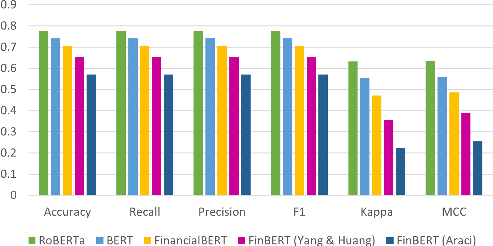
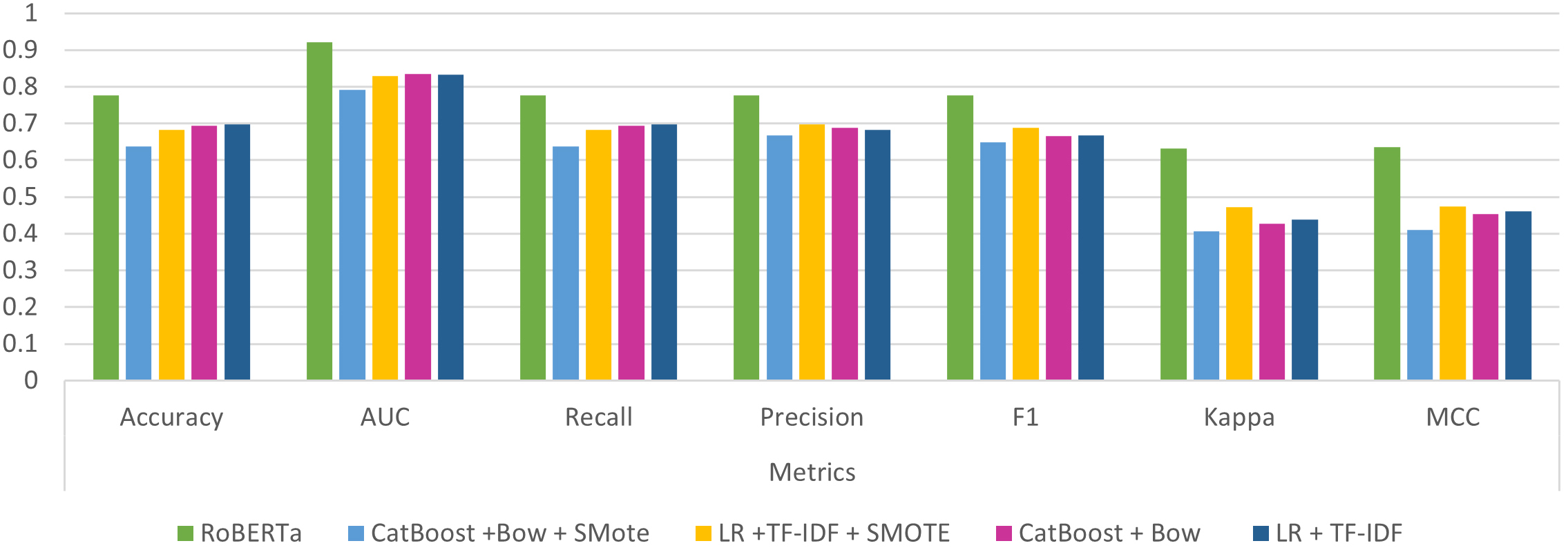
Regarding Deep Learning Pre-Trained models, RoBERTa exhibits a remarkable performance, outperforming all other models across all metrics. The BERT model follows in second place, while FiancialBERT and FinBERT (Yang & Hung) secure the third and fourth positions, respectively. FinBERT (Araci) can be found in the last place, considering all metrics. The indisputable dominance of RoBERTa is evident, as it consistently achieves superior scores, surpassing competitors by margins ranging from 2% to 7% in different metrics, as indicated in Table 6. It’s worth noting that ROC-AUC values for the FinBERT models could not be obtained due to the absence of necessary class probabilities from these models, which are crucial for calculating this metric. The corresponding results for all metrics are also depicted with a graphical representation of them, which can be found in Fig. 3. The AUC metric is excluded, as it could not be calculated for FinBERT models, due model limitations.
Figure 3.
Deep learning pre-trained models’ performance.
4.1.6General discussion
The design of the experimental procedure was thoughtfully structured to offer valuable insights into several distinct inquiries. The primary focus revolves around comparing the utilization of Deep Learning Pre-Trained Models and classic ML models, with a particular emphasis on assessing whether integrating more sophisticated models translates to improved performance. Within the domain of traditional ML models, two pivotal questions come to the forefront.
Firstly, there is the question of choosing between BoW and TF-IDF techniques, aiming to discern which among them yields more favorable outcomes. This inquiry directly concerns word representation, investigating which technique better captures the nuances of language and ultimately contributes to superior model performance.
Secondly, an additional aspect under scrutiny is the potential benefit derived from employing the SMOTE technique to artificially augment our data in order to tackle the problem of the initial imbalanced dataset. This question delves into the interplay between model performance and the integration of SMOTE, seeking to uncover whether the introduction of this technique positively impacts the final outcomes of the models.
Through a comprehensive exploration of these questions, the experimental design seeks to shed light on the intricate dynamics between various modelling approaches, offering nuanced insights into the strengths and limitations of each technique and aiding in informed decision-making for optimal model selection. To give a better insight into the results, in Fig. 4, the results of the five single best methods (according to MCC) are given in a graphical representation.
Table 6
Deep learning pre-trained models’ performance
| Model | Accuracy | AUC | Recall | Precision | F1 | Kappa | MCC |
|---|---|---|---|---|---|---|---|
| RoBERTa | 0.775877 | 0.920793 | 0.775877 | 0.775877 | 0.775877 | 0.632183 | 0.634966 |
| BERT | 0.74166 | 0.89992 | 0.74166 | 0.74166 | 0.74166 | 0.554974 | 0.558077 |
| FinalcialBERT | 0.704876 |
| 0.704876 | 0.704876 | 0.704876 | 0.47108 | 0.486317 |
| FinBERT (Yang & Huang) | 0.65355 |
| 0.65355 | 0.65355 | 0.65355 | 0.355566 | 0.389141 |
| FinBERT (Araci) | 0.570573 |
| 0.570573 | 0.570573 | 0.570573 | 0.224854 | 0.256037 |
Figure 4.
Best 5 single classic ML methods.
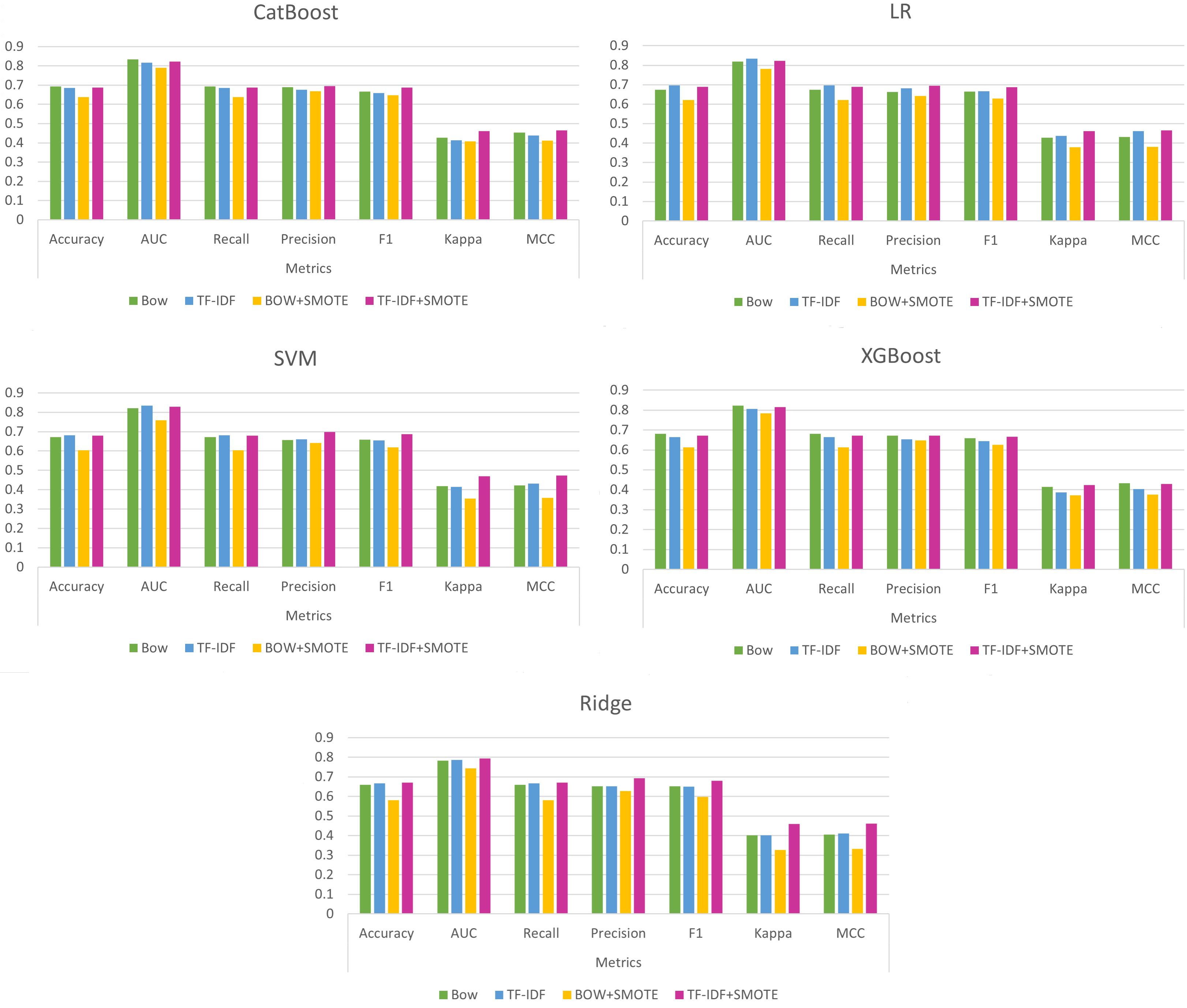
Regarding the initial question, the results do not provide a definitive answer. Concerning the utilization of BoW or TF-IDF (when SMOTE is not applied), it appears that in certain methods, such as Catboost and XGBoost, BoW exhibits superior performance, while in others, TF-IDF proves to be more effective. However, when SMOTE is applied, TF-IDF outperforms BoW, notably enhancing performance across all metrics.
Turning to the second question, which pertains to the potential advantages of utilizing SMOTE, the answer becomes quite evident. When employing BoW, using SMOTE tends to lead to a reduction in model performance across all metrics. In certain instances, such as when employing the Ridge Classifier, this decline in performance is notably significant. On the other hand, when TF-IDF is employed, the results provide a clear picture. Specifically, in terms of Precision, F1 Score, Kappa, and MCC, the outcomes unambiguously indicate that SMOTE enhances model performance. However, when considering metrics like accuracy, AUC, and Recall, the situation becomes less straightforward. While in the majority of cases, the utilization of SMOTE proves beneficial, there are instances where its application appears to have a minor detrimental effect on model performance in these three metrics.
Regarding the utilization of ensemble techniques, it is important to note two key observations. First and foremost, ensembles generally tend to outperform the vast majority of individual ML models. However, it is worth noting that they do not surpass the best-performing single method in each specific scenario, except the AUC metric, where ensembles consistently outperform single methods across all cases. Our findings confirm the overall strong performance of ensembles. However, in the context of our study, their contribution is not particularly significant, and they may not be the preferred choice. It is worth mentioning that the tested ensembles were soft voting schemes. More sophisticated ensemble techniques may have the potential to be more powerful and possibly yield better results.
As we arrive at the final point of our findings, which pertains to the overall performance of classical ML classification algorithms compared to sophisticated Deep Learning Pre-Trained models, the outcome appears quite promising. Deep Learning Pre-Trained models consistently outperform their classic counterparts across all metrics. To be more specific, regarding the best-performing pre-trained model, RoBERTa, and the top single model from each of the four classical ML scenarios, RoBERTa showcases a substantial improvement in every metric. For example, RoBERTa achieves a 7% higher accuracy compared to the following method, which combines Logistic Regression (LR) with TF-IDF. In terms of the MCC metric, the results are even more compelling, with RoBERTa once again outperforming its closest rival by a margin of 17%. In Fig. 5, the corresponding results of all metrics are depicted.
Figure 5.
RoBERTa vs the best single classifier of each scenario.
However, it is worth noting an unexpected yet valuable outcome: both RoBERTa and BERT outperform the three variants of FinBERT. This discovery raises intriguing questions and warrants further investigation, especially considering that FinBERT models are fine-tuned specifically for financial tasks.
5.Conclusions
In this work, a large number of classic ML algorithms is tested against five contemporary Deep Learning PreTrained models. Specifically, fifteen well-known, traditional ML classification methods drawn from the Pycaret python library are used. Four different scenarios are tested, using two different text representation techniques (BoW and TF-IDF) and employing (or not) SMOTE data augmentation technique to balance our initially imbalanced dataset. Concerning these factors, four variants of each classification method are formed (BoW, TF-IDF, BoW
The analysis of the results has unveiled several intriguing findings, some of which align with expectations while others come as surprises. First and foremost, the unquestionable supremacy of pre-trained models is evident, with RoBERTa and BERT emerging as the top-performing methods. However, this leads to one of the unexpected revelations in this study: the three variants of FinBERT, despite being tailored for financial tasks, do not outperform BERT and RoBERTa. This intriguing outcome underscores the need for further investigation and future research to shed light on this matter. Turning our attention to the variants of traditional machine learning classification algorithms and their ensembles, when SMOTE is applied, the TF-IDF versions of classifiers outperform their BoW counterparts. Furthermore, with respect to SMOTE utilization, it is evident that it notably enhances performance when combined with TF-IDF while also yielding improvements in most metrics when paired with BoW.
Regarding potential future extensions of this study, exploring ensembles consisting of classic and contemporary pre-trained models is advisable. This concept aligns with ensemble theory, emphasizing the importance of accurate and diverse base methods within an ensemble. Additionally, exploring more sophisticated ensemble schemes should be considered and empirically tested. Another noteworthy aspect arising from the results is the need for further investigation into the performance of FinBERT models. Their performance, ranking below general-purpose models, defies initial expectations and merits deeper scrutiny to understand the factors at play better.
References
[1] | Zhang L, Liu B. Sentiment Analysis and Opinion Mining. Encyclopedia of Machine Learning and Data Mining. (2017) ; 1: : 1152-61. |
[2] | Yang L, Li Y, Wang J, Sherratt RS. Sentiment Analysis for E-Commerce Product Reviews in Chinese Based on Sentiment Lexicon and Deep Learning. IEEE Access. (2020) ; 82: : 3522-30. |
[3] | Harish BS, Kumar K, Darshan HK. Sentiment Analysis on IMDb Movie Reviews Using Hybrid Feature Extraction Method. International Journal of Interactive Multimedia and Artificial Intelligence. (2019) ; 06/2019; 5: (5): 109-14. Available from: https//www.ijimai.org/journal/sites/default/files/files/2018/12/ijimai_5_5_13_pdf_67503.pdf. |
[4] | Shaukat Z, Zulfiqar AA, Xiao C, Azeem M, Mahmood T. Sentiment analysis on IMDB using lexicon and neural networks. SN Applied Sciences. (2020) Jan; 2: (2): 148. Available from: doi: 10.1007/s42452-019-1926-x. |
[5] | Ortigosa A, Martín JM, Carro RM. Sentiment analysis in Facebook and its application to e-learning. Computers in Human Behavior. (2014) ; 31: : 527-41. Available from: https//www.sciencedirect.com/science/article/pii/S0747563213001751. |
[6] | Thelwall MA. Social media analytics for YouTube comments: potential and limitations. International Journal of Social Research Methodology. (2018) ; 21: : 303; 316. Available from: https//api.semanticscholar.org/CorpusID:148591270. |
[7] | Jianqiang Z, Xiaolin G, Xuejun Z. Deep Convolution Neural Networks for Twitter Sentiment Analysis. IEEE Access. (2018) ; 6: : 23253-60. |
[8] | Zimbra D, Abbasi A, Zeng D. The State-of-the-Art in Twitter Sentiment Analysis: A Review and Benchmark Evaluation. ACM Transactions on Management Information Systems. (2018) ; 05; xx, No. x. |
[9] | Kumar A, Jaiswal A. Systematic literature review of sentiment analysis on Twitter using soft computing techniques. Concurrency and Computation: Practice and Experience. (2020) ; 32: (1): e5107; E5107 CPE-18-1167.R1. Available from: doi: 10.1002/cpe.5107. |
[10] | Xu QA, Chang V, Jayne C. A systematic review of social media-based sentiment analysis: Emerging trends and challenges. Decision Analytics Journal. (2022) ; 3: : 10007; Available from: https//www.sciencedirect.com/science/article/pii/S2772662222000273. |
[11] | Korkontzelos I, Nikfarjam A, Shardlow M, Sarker A, Ananiadou S, Gonzalez G. Analysis of the effect of sentiment analysis on extracting adverse drug reactions from tweets and forum posts. Journal of Biomedical Informatics. (2016) ; 06: ; 62. |
[12] | Liu J, Zhao S, Zhang X. An ensemble method for extracting adverse drug events from social media. Artificial intelligence in medicine. (2016) ; 70: : 62-76 Available from: https//api.semanticscholar.org/CorpusID:205694936. |
[13] | Peng Y, Yan S, Lu Z. Transfer Learning in Biomedical Natural Language Processing: An Evaluation of BERT and ELMo on Ten Benchmarking Datasets. In: Proceedings of the 18th BioNLP Workshop and Shared Task. Florence, Italy: Association for Computational Linguistics; (2019) . p. 58-65. Available from: https//aclanthology.org/W19-5006. |
[14] | Zunic A, Corcoran P, Spasic I. Sentiment Analysis in Health and Well-Being: Systematic Review. JMIR Med Inform. (2020) Jan; 8: (1): e16023. Available from: http//www.ncbi.nlm.nih.gov/pubmed/32012057. |
[15] | Chauhan P, Sharma N, Sikka G. The emergence of social media data and sentiment analysis in election prediction. Journal of Ambient Intelligence and Humanized Computing. (2020) ; 12: : 2601-27. Available from: https//api.semanticscholar.org/CorpusID:225442640. |
[16] | Santos J, Bernardini F, Paes A. A survey on the use of data and opinion mining in social media to political electoral outcomes prediction. Social Network Analysis and Mining. (2021) ; 12: ; 11. |
[17] | Rita P, Antonio N, Afonso A. Social media discourse and voting decisions influence: sentiment analysis in tweets during an electoral period. Social Network Analysis and Mining. (2023) ; 03: : 13. |
[18] | Beigi G, Hu X, Maciejewski R, Liu H. An overview of sentiment analysis in social media and its applications in disaster relief. Sentiment Analysis and Ontology Engineering: An Environment of Computational Intelligence. (2016) ; 313-40. |
[19] | Birjali M, Beni-Hssane A, Erritali M. Machine Learning and Semantic Sentiment Analysis based Algorithms for Suicide Sentiment Prediction in Social Networks. Procedia Computer Science. (2017) ; 113: : 65-72; The 8th International Conference on Emerging Ubiquitous Systems and Pervasive Networks (EUSPN 2017)/The 7th International Conference on Current and Future Trends of Information and Communication Technologies in Healthcare (ICTH-2017)/Affiliated Workshops. Available from: https//www.sciencedirect.com/science/article/pii/S187705091731699X. |
[20] | Swain D, Khandelwal A, Joshi C, Gawas A, Roy P, Zad V. A Suicide Prediction System Based on Twitter Tweets Using Sentiment Analysis and Machine Learning. In: Swain D, Pattnaik PK, Athawale T, editors. Machine Learning and Information Processing. Singapore: Springer Singapore (2021) ; pp. 45-58. |
[21] | Rambocas M, Pacheco B. Online sentiment analysis in marketing research: a review. Journal of Research in Interactive Marketing. (2018) ; 01: : 12. |
[22] | Yousif A, Niu Z, Tarus JK, Ahmad A. A Survey on Sentiment Analysis of Scientific Citations. Artificial Intelligence Review. (2019) Oct; 52: (3): 1805-1838. Available from: doi: 10.1007/s10462-017-9597-8. |
[23] | Alaei AR, Becken S, Stantic B. Sentiment Analysis in Tourism: Capitalizing on Big Data. Journal of Travel Research. (2019) ; 58: (2): 175-91. Available from: doi: 10.1177/0047287517747753. |
[24] | Seki K, Ikuta Y. S-APIR: News-based Business Sentiment Index. ArXiv. 2020abs/2003.02973. Available from: https//api.semanticscholar.org/CorpusID:212628659. |
[25] | Seki K, Ikuta Y, Matsubayashi Y. News-based business sentiment and its properties as an economic index. Information Processing & Management. (2022) ; 59: (2): 102795. Available from: https//www.sciencedirect.com/science/article/pii/S0306457321002739. |
[26] | Xing F, Cambria E, Welsch RE. Natural language based financial forecasting: a survey. Artificial Intelligence Review. (2017) ; 50: : 49-73. Available from: https//api.semanticscholar.org/CorpusID:207079655. |
[27] | Mäntylä MV, Graziotin D, Kuutila M. 4The evolution of sentiment analysis – A review of research topics, venues, and top cited papers. Computer Science Review. (2018) ; 27: : 16-32; Available from: https//www.sciencedirect.com/science/article/pii/S1574013717300606. |
[28] | Ren R, Wu DD, Liu T. Forecasting Stock Market Movement Direction Using Sentiment Analysis and Support Vector Machine. IEEE Systems Journal. (2019) ; 13: : 760-70. Available from: https//api.semanticscholar.org/CorpusID:67870584. |
[29] | Papaioannou P, Russo L, Papaioannou G, Siettos CI. Can social microblogging be used to forecast intraday exchange rates? NETNOMICS: Economic Research and Electronic Networking. (2013) ; 14: : 47-68; Available from: https//api.semanticscholar.org/CorpusID:2516894. |
[30] | Deveikyte J, Geman H, Piccari C, Provetti A. A sentiment analysis approach to the prediction of market volatility. Frontiers in Artificial Intelligence. (2022) ; 5: . Available from: https//www.frontiersin.org/articles/10.3389/frai.2022.836809. |
[31] | Malandri L, Xing F, Orsenigo C, Vercellis C, Cambria E. Public Mood–Driven Asset Allocation: the Importance of Financial Sentiment in Portfolio Management. Cognitive Computation. (2018) ; 10: : 1167-76; Available from: https//api.semanticscholar.org/CorpusID:53795790. |
[32] | Xing FZ, Cambria E, Welsch RE. Intelligent Asset Allocation via Market Sentiment Views. IEEE Computational Intelligence Magazine. (2018) ; 13: (4): 25-34. |
[33] | Zhang D, Xu W, Zhu Y, Zhang X. Can Sentiment Analysis Help Mimic Decision-Making Process of Loan Granting? A Novel Credit Risk Evaluation Approach Using GMKL Model. 2015 48th Hawaii International Conference on System Sciences. (2015) : 949-58. Available from: https//api.semanticscholar.org/CorpusID:17733609. |
[34] | Bajo E, Raimondo C. Media sentiment and IPO underpricing. Journal of Corporate Finance. (2017) ; 46: : 139-53; Available from: https//www.sciencedirect.com/science/article/pii/S092911991730370X. |
[35] | Kraaijeveld O, De Smedt J. The predictive power of public Twitter sentiment for forecasting cryptocurrency prices. Journal of International Financial Markets, Institutions and Money. (2020) ; 65: : 101188; Available from: https//www.sciencedirect.com/science/article/pii/S104244312030072X. |
[36] | Rognone L, Hyde S, Zhang SS. News sentiment in the cryptocurrency market: An empirical comparison with Forex. International Review of Financial Analysis. (2020) ; 69: (C). |
[37] | Aslam N, Rustam F, Lee E, Washington PB, Ashraf I. Sentiment Analysis and Emotion Detection on Cryptocurrency Related Tweets Using Ensemble LSTM-GRU Model. IEEE Access. (2022) Jan. |
[38] | Mardjo A, Choksuchat C. HyVADRF: Hybrid VADER–Random Forest and GWO for Bitcoin Tweet Sentiment Analysis. IEEE Access. (2022) ; 10: : 101889-97. |
[39] | Xing F, Malandri L, Zhang Y, Cambria E. Financial Sentiment Analysis: An Investigation into Common Mistakes and Silver Bullets. In: Proceedings of the 28th International Conference on Computational Linguistics. Barcelona, Spain (Online): International Committee on Computational Linguistics; (2020) . pp. 978-87. Available from: https//aclanthology.org/2020.coling-main.85. |
[40] | Wankhade M, Rao ACS, Kulkarni C. A survey on sentiment analysis methods, applications, and challenges. Artificial Intelligence Review. (2022) Oct; 55: (7): 5731-80. Available from: doi: 10.1007/10462-022-10144-1. |
[41] | Tetlock PC. Giving Content to Investor Sentiment: The Role of Media in the Stock Market. The Journal of Finance. (2007) ; 62: (3): 1139-68; Available from: doi: 10.1111/j.1540-6261.2007.01232.x. |
[42] | Loughran T, Mcdonald B. When Is a Liability Not a Liability? Textual Analysis, Dictionaries, and 10-Ks. The Journal of Finance. (2011) ; 66: (1): 35-65. Available from: doi: 10.1111/j.1540-6261.2010.01625.x. |
[43] | Yekrangi M, Abdolvand N. Financial markets sentiment analysis: developing a specialized Lexicon. Journal of Intelligent Information Systems. (2021) Aug; 57: (1): 127-46. Available from: doi: 10.1007/s10844-020-00630-9. |
[44] | Bos T, Frasincar F. Automatically Building Financial Sentiment Lexicons While Accounting for Negation. Cognitive Computation. (2021) ; 14: : 442-60; Available from: https//api.semanticscholar.org/CorpusID:233890630. |
[45] | Consoli S, Barbaglia L, Manzan S. Fine-Grained, Aspect-Based Sentiment Analysis on Economic and Financial Lexicon. WGSRN: Data Collection & Empirical Methods (Topic). 2021. Available from: https//api.semanticscholar.org/CorpusID:233755615. |
[46] | Malo P, Sinha A, Korhonen PJ, Wallenius J, Takala P. Good debt or bad debt: Detecting semantic orientations in economic texts. Journal of the Association for Information Science and Technology. (2013) ; 65: ; Available from: https//api.semanticscholar.org/CorpusID:7700237. |
[47] | Mishev K, Gjorgjevikj A, Vodenska I, Chitkushev LT, Trajanov D. Evaluation of Sentiment Analysis in Finance: From Lexicons to Transformers. IEEE Access. (2020) ; 8: : 131662-82; Available from: https//api.semanticscholar.org/CorpusID:220836326. |
[48] | Maia M, Freitas A, Handschuh S. FinSSLx: A Sentiment Analysis Model for the Financial Domain Using Text Simplification 2018 IEEE 12th International Conference on Semantic Computing (ICSC). (2018) : 318-9. Available from: https//api.semanticscholar.org/CorpusID:4884174. |
[49] | Chiong R, Fan Z, Hu Z, Adam MTP, Lutz B, Neumann D. A sentiment analysis-based machine learning approach for financial market prediction via news disclosures. Proceedings of the Genetic and Evolutionary Computation Conference Companion. (2018) ; Available from: https//api.semanticscholar.org/CorpusID:49668701. |
[50] | Sharma V, Khemnar RK, Kumari RA, Mohan BR. Time Series with Sentiment Analysis for Stock Price Prediction 2019 2nd International Conference on Intelligent Communication and Computational Techniques (ICCT). (2019) : 178-81. Available from: https//api.semanticscholar.org/CorpusID:210971954. |
[51] | Koukaras P, Nousi C, Tjortjis C. Stock Market Prediction Using Microblogging Sentiment Analysis and Machine Learning. Telecom. (2022) ; Available from: https//api.semanticscholar.org/CorpusID:249248047. |
[52] | Valencia F, Gómez-Espinosa A, Valdés-Aguirre B. Price Movement Prediction of Cryptocurrencies Using Sentiment Analysis and Machine Learning. Entropy. (2019) ; 21; Available from: https//api.semanticscholar.org/CorpusID:195825545. |
[53] | Liapis CM, Karanikola A, Kotsiantis SB. A Multi-Method Survey on the Use of Sentiment Analysis in Multivariate Financial Time Series Forecasting. Entropy. (2021) ; 23; Available from: https//api.semanticscholar.org/CorpusID:245444145. |
[54] | Sohangir S, Wang D, Pomeranets A, Khoshgoftaar TM. Big Data: Deep Learning for financial sentiment analysis. Journal of Big Data. (2018) ; 5: : 1-25; Available from: https//api.semanticscholar.org/CorpusID:4033865. |
[55] | Xu Y, Keselj V. Stock Prediction using Deep Learning and Sentiment Analysis 2019 IEEE International Conference on Big Data (Big Data). (2019) ; 5573-80. Available from: https//api.semanticscholar.org/CorpusID:211298482. |
[56] | Passalis N, Avramelou L, Seficha S, Tsantekidis A, Doropoulos S, Makris G, et al. Multisource financial sentiment analysis for detecting Bitcoin price change indications using deep learning. Neural Computing and Applications. (2022) ; 34: : 19441-19452. Available from: https//api.semanticscholar.org/CorpusID:250272176. |
[57] | Raju SM, Tarif AM. Real-Time Prediction of BITCOIN Price using Machine Learning Techniques and Public Sentiment Analysis. ArXiv. (2020) ; abs/2006.14473. Available from: https//api.semanticscholar.org/CorpusID:220056249. |
[58] | Liapis CM, Karanikola A, Kotsiantis SB. Investigating Deep Stock Market Forecasting with Sentiment Analysis. Entropy. (2023) ; 25; Available from: https//api.semanticscholar.org/CorpusID:256296957. |
[59] | Zhang L, Wang S, Liu B. Deep learning for sentiment analysis: A survey. Wiley Interdisciplinary Reviews: Data Mining and Knowledge Discovery. (2018) ; 8; Available from: https//api.semanticscholar.org/CorpusID:10694510. |
[60] | Yadav A, Vishwakarma DK. Sentiment analysis using deep learning architectures: a review. Artificial Intelligence Review. (2019) ; 53: : 4335-4385. Available from: https//api.semanticscholar.org/CorpusID:208539187. |
[61] | Ozbayoglu AM, Gudelek MU, Sezer OB. Deep Learning for Financial Applications: A Survey. Appl Soft Comput. (2020) ; 93: : 106384; Available from: https//api.semanticscholar.org/CorpusID:211126927. |
[62] | Gutiérrez-Fandiño A, Kolm PN, i Alonso MN, Armengol-Estapé J. FinEAS: Financial Embedding Analysis of Sentiment. The Journal of Financial Data Science. (2022) ; 4: (3): 45-53. |
[63] | Araci D. FinBERT: Financial Sentiment Analysis with Pre-trained Language Models. ArXiv. (2019) ; abs/1908. 10063. Available from: https//api.semanticscholar.org/CorpusID:201646244. |
[64] | DeSola V, Hanna K, Nonis P. Finbert: pre-trained model on sec filings for financial natural language tasks. University of California. (2019) . |
[65] | Liu Z, Huang D, Huang K, Li Z, Zhao J. Finbert: A pre-trained financial language representation model for financial text mining. In: Proceedings of the twenty-ninth international conference on international joint conferences on artificial intelligence; (2021) ; pp. 4513-9. |
[66] | Yang Y, Uy MCS, Huang A. FinBERT: A Pretrained Language Model for Financial Communications. ArXiv.2020abs/ 2006.08097. Available from: https//api.semanticscholar.org/CorpusID:219687757. |
[67] | Huang A, Wang H, Yang Y. FinBERT: A Large Language Model for Extracting Information from Financial Text. Contemporary Accounting Research. (2022) ; Available from: https//api.semanticscholar.org/CorpusID:252666016. |
[68] | Agarwal B. Financial sentiment analysis model utilizing knowledge-base and domain-specific representation. Multimedia Tools and Applications. (2022) ; 82: : 8899-920; Available from: https//api.semanticscholar.org/CorpusID:246849870. |
[69] | Financial Sentiment Analysis – kaggle.com; [Accessed 29-09-2023]. https://www.kaggle.com/datasets/sbhatti/financial-sentiment-analysis. |
[70] | Maia M, Handschuh S, Freitas A, Davis B, McDermott R, Zarrouk M, et al. WWW’18 Open Challenge: Financial Opinion Mining and Question Answering. Companion Proceedings of the The Web Conference. (2018) ; 2018. Available from: https//api.semanticscholar.org/CorpusID:13866508. |
[71] | Malo P, Sinha A, Takala P, Korhonen P, Wallenius J. FinancialPhraseBank-v1.0; (2013) . |
[72] | Lexis Nexis Database; [Accessed 29-09-2023]. https://www.lexisnexis.com/en-us/home.page. |
[73] | Chai CP. Comparison of text preprocessing methods. Natural Language Engineering. (2022) ; 29: : 509-553. Available from: https//api.semanticscholar.org/CorpusID:249657675. |
[74] | HaCohen-Kerner Y, Miller D, Yigal Y. The influence of preprocessing on text classification using a bag-of-words representation. PLoS ONE. (2020) ; 15; Available from: https//api.semanticscholar.org/CorpusID:218479987. |
[75] | Ali M. PyCaret: An open source, low-code machine learning library in Python; 2020. PyCaret version 1.0.0. Available from: https//www.pycaret.org. |
[76] | Akuma S, Lubem T, Adom IT. Comparing Bag of Words and TF-IDF with different models for hate speech detection from live tweets. International Journal of Information Technology. (2022) ; Available from: https//api.semanticscholar.org/CorpusID:252449382. |
[77] | Flores AC, Icoy RI, Peña CF, Gorro K. An Evaluation of SVM and Naive Bayes with SMOTE on Sentiment Analysis Data Set 2018 International Conference on Engineering, Applied Sciences, and Technology (ICEAST). (2018) ; 1-4. Available from: https//api.semanticscholar.org/CorpusID:52014088. |
[78] | Satriaji W, Kusumaningrum R. Effect of Synthetic Minority Oversampling Technique (SMOTE), Feature Representation, and Classification Algorithm on Imbalanced Sentiment Analysis 2018 2nd International Conference on Informatics and Computational Sciences (ICICoS). (2018) : 1-5. Available from: https//api.semanticscholar.org/CorpusID:59231725. |
[79] | Chicco D, Jurman G. The advantages of the Matthews correlation coefficient (MCC) over F1 score and accuracy in binary classification evaluation. BMC Genomics. (2020) ; 21; Available from: https//api.semanticscholar.org/CorpusID:209528322. |
[80] | Athar A, Ali S, Sheeraz MM, Bhattacharjee S, Kim H. Sentimental Analysis of Movie Reviews using Soft Voting Ensemble-based Machine Learning 2021 Eighth International Conference on Social Network Analysis, Management and Security (SNAMS). 2021: : 01-5. Available from: https//api.semanticscholar.org/CorpusID:247477419. |
[81] | Wan Y, Gao Q. An Ensemble Sentiment Classification System of Twitter Data for Airline Services Analysis 2015 IEEE International Conference on Data Mining Workshop (ICDMW). (2015) : 1318-25. Available from: https//api.semanticscholar.org/CorpusID:21442. |
[82] | Devlin J, Chang MW, Lee K, Toutanova K. Bert: Pre-training of deep bidirectional transformers for language understanding. arXiv preprint arXiv181004805. (2018) . |
[83] | Vaswani A, Shazeer N, Parmar N, Uszkoreit J, Jones L, Gomez AN, et al. Attention is all you need. Advances in Neural Information Processing Systems. (2017) ; 30. |
[84] | Lee CC, Gao Z, Tsai CL. BERT-Based Stock Market Sentiment Analysis 2020 IEEE International Conference on Consumer Electronics – Taiwan (ICCE-Taiwan). (2020) : 1-2. Available from: https//api.semanticscholar.org/CorpusID:227220140. |
[85] | Soong GH, Tan CC. Sentiment Analysis on 10-K Financial Reports using Machine Learning Approaches 2021 IEEE 11th International Conference on System Engineering and Technology (ICSET). (2021) ; 124-9. Available from: https//api.semanticscholar.org/CorpusID:244778394. |
[86] | Liu Y, Ott M, Goyal N, Du J, Joshi M, Chen D, et al. RoBERTa: A Robustly Optimized BERT Pretraining Approach. ArXiv. (2019) ; abs/1907.11692. Available from: https//api.semanticscholar.org/CorpusID:198953378. |
[87] | Bozanta A, Angco S, Cevik M, Basar A. Sentiment Analysis of StockTwits Using Transformer Models 2021 20th IEEE International Conference on Machine Learning and Applications (ICMLA). (2021) : 1253-8. Available from: https//api.semanticscholar.org/CorpusID:246289092. |
[88] | Sinha A, Kedas S, Kumar R, Malo P. SEntFiN 10: Entity-aware sentiment analysis for financial news. Journal of the Association for Information Science and Technology. (2022) ; 73: : 1314-1335. Available from: https//api.semanticscholar.org/CorpusID:247341717. |
[89] | Gupta A, Tayal VK. Analysis of Twitter Sentiment to Predict Financial Trends 2023 International Conference on Artificial Intelligence and Smart Communication (AISC). (2023) : 1027-31. Available from: https//api.semanticscholar.org/CorpusID:257930671. |
[90] | Krishnamoorthy S. Sentiment analysis of financial news articles using performance indicators. Knowledge and Information Systems. (2018) ; 56: : 373-94; Available from: https//api.semanticscholar.org/CorpusID:32437011. |
[91] | ProsusAI Finbert Model; [Accessed 29-09-2023]. https//huggingface.co/ProsusAI/finbert. |
[92] | psnonis. FinBERT model; [Accessed 29-09-2023]. https//github.com/psnonis/FinBERT. |
[93] | yiyanghkust. finbert-tone model; [Accessed 29-09-2023]. https//huggingface.co/yiyanghkust/finbert-tone. |
[94] | Hazourli A. Financialbert-a pretrained language model for financial text mining. Technical Report. (2022) . |
[95] | Hazourli A. ahmedrachid/FinancialBERT; 2022. [Accessed 29-09-2023]. https//huggingface.co/ahmedrachid/FinancialBERT. |
[96] | Kingma DP, Ba J. Adam: A Method for Stochastic Optimization. CoRR. (2014) ; abs/1412.6980. Available from: https//api.semanticscholar.org/CorpusID:6628106. |

