
How graph features from message passing affect graph classification and regression?
Abstract
Graph neural networks (GNNs) have been applied to various graph domains. However, GNNs based on the message passing scheme, which iteratively aggregates information from neighboring nodes, have difficulty learning to represent larger subgraph structures because of the nature of the scheme. We investigate the prediction performance of GNNs when the number of message passing iteration increases to capture larger subgraph structures on classification and regression tasks using various real-world graph datasets. Our empirical results show that the averaged features over nodes obtained by the message passing scheme in GNNs are likely to converge to a certain value, which significantly deteriorates the resulting prediction performance. This is in contrast to the state-of-the-art Weisfeiler–Lehman graph kernel, which has been used actively in machine learning for graphs, as it can comparably learn the large subgraph structures and its performance does not usually drop significantly drop from the first couple of rounds of iterations. Moreover, we report that when we apply node features obtained via GNNs to SVMs, the performance of the Weisfeiler-Lehman kernel can be superior to that of the graph convolutional model, which is a typically employed approach in GNNs.
1.Introduction
Graph-structured data are ubiquitous in various domains from social networks to system engineering and bio- and chemo-informatics. Most of the recent machine learning methods for graphs are essentially based on the message passing scheme, which aggregates feature vectors associated with neighboring nodes and updates them via a certain function at each node [1, 2, 3, 4, 5]. This scheme is widely employed to learn the representation of nodes and graphs in recently proposed graph neural networks (GNNs).
In machine learning on graphs, graph kernels have been studied to measure the similarity between graphs, which can be combined with classification or prediction tasks to achieve good predictive performances on various graph datasets [6, 7, 8]. If node features in graphs are discrete – that is, each node has its label – the Weisfeiler–Lehman (WL) sub-tree graph kernel can be the first choice for graph classification tasks, which also shares the message passing algorithm in its process [9]. This “WL scheme” can effectively and efficiently count subgraph patterns in graphs, resulting in the high predictive performance in ML tasks for graphs. The WL scheme obtains feature vectors based on counting the node label appearance on neighboring nodes, which implicitly obtains representation of graphs and is likely to represent some specific characteristics that are able to explain targets in graph ML tasks. Although huge computational cost is a limitation of graph kernel approaches, the quadratic time complexity with respect to the number of graphs in construction of a kernel matrix, when applied to larger datasets, make their performance superior to other approaches in various medium sized datasets [6].
GNNs have emerged as a way of learning representation on graphs. The message passing scheme is commonly used in most of proposed GNNs [2, 4, 10, 11]. For example, graph convolutional network (GCN) is known to be a simple GNN model for semi-supervised learning [10], which is similar to the WL scheme. Graph isomorphism network (GIN) is more similar to the WL graph kernel, which have been theoretically and empirically shown to be as powerful as the WL scheme with respect to their discriminability and representation power [2]. In addition, to learn better representation of node features and overcome the limitation of graph convolutions, attention-based graph neural models have been studied [3, 12]. These graph neural network models are helpful to solve graph prediction tasks as well as node or link prediction.
In GNNs, the problem of over-smoothing, where the similarity between nodes becomes closer and closer when more and more message passing is performed, is one of common issues. The over-smoothing deteriorates the quality of graph representation, particularly when multiple convolutional layers are stacked, because of the low information-to-noise ratio of the message received by the nodes, which is partially determined by the graph topology [13]. As a result, the performance of a trained model such as the accuracy of classification worsens when over-smoothing occurs. This means that the message passing scheme may inherently have a limitation in terms of capturing large subgraph structures as it requires many message passing iterations. Thus, if such large subgraphs are relevant in prediction, this would be a serious problem for GNNs.
In this paper, to investigate the advantage and the limitation of the message passing scheme in GNNs and graph kernels, we focus on the influence of the over-smoothing problem. More precisely, we empirically examine how features of graph substructures obtained by the WL (or message passing) scheme affect the predictive performance as the number of convolutional layers increases. First, we compare the WL sub-tree graph kernels with GNNs, including GCNs and GINs on classification and regression real-world graph datasets collected from a variety of domains. In GNNs, for certain types of datasets, we show that the large number of message passing iterations deteriorates the predictive performance due to the over-smoothing phenomenon. Second, we argue that the averaged feature vectors over nodes learned from graph convolutional layers, which are expected to represent the overall graph characteristics, are not stable as the number of message passing iterations increases. Finally, we evaluate graph features on multi-layer perceptrons (MLPs) and support vector machines (SVMs) in the task of classification and regression. We also show that SVMs with features obtained from GCNs can be used as a way of measuring how strong the contribution of node features is, where the node features are concatenated at each message passing iteration.
Our contributions are summarized as follows:
• The prediction performance of the WL kernel outperforms the most fundamental GNNs, GCNs and GINs, if the number of message passing iteration increases.
• The WL kernel does not deteriorate significantly for many message passing iterations in most of datasets, while GCNs and GINs do deteriorate due to their large number of parameters and ill-trained previous node features.
• Transition of node features tend to be small, which leads to difficulty of determining which feature is informative for prediction, and the features converge to indistinguishable values when the training fails.
2.Methods for graph machine learning
2.1Notation
A graph is a tuple
For two graphs
2.2The vertex histogram kernel
One of the simplest graph kernels is the vertex histogram kernel, which counts node label matching between a pair of graphs. Let
(1)
2.3The Weisfeiler–Lehman Kernel
The Weisfeiler–Lehman (WL) sub-tree kernel is based on the Weisfeiler–Lehman test of isomorphism. The key idea of the kernel is the “WL scheme”, which is re-labeling of node labels by gathering neighboring node labels. Then each new label is a good proxy of an indicator of subgraph structure. This re-labeling step is repeated until every pair of graphs have different node labels or reaching at a certain step
In the WL kernels, these subgraph structures obtained from the WL scheme are mapped into the Hilbert space. In other words, the obtained node label sets are used to compute the similarity between graphs. The WL kernel is also based on the vertex histogram, but it extends the original vertex histogram through iterations of node re-labeling. The final kernel matrix after
(2)
where
(3)
where
2.4Graphlet kernel
The graphlet kernel is calculated by the frequency of occurrence of matched subgraphs, called graphlets [14]. Graphs are decomposed into graphlets. Let
(4)
2.5Graph convolutional neural networks
Graph convolutional neural networks are first introduced for semi-supervised learning of classifying nodes in a graph. In graph convolutional networks, node labels are treated as a feature matrix
(5)
where
For regression and classification settings, the output of node features at the final layer is reduced by the pooling operation, such as taking the mean and the sum over vertices, which is equivalent to the readout operation that can obtain the representation of graph features. The readout graph feature is passed into MLP layers and trained through back propagation.
In computing for classification and regression, the reduce function that returns the final output value
(6)
where READOUT
2.6Graph isomorphism networks
The graph isomorphism network (GIN) is a model that is known to be as powerful as the WL test [2]. To update the representation of each node feature vector
(7)
where
(8)
The READOUT function aggregates node features from the final iteration to obtain graph features of
(9)
where
2.7Special case of GIN (Pre-fixed GCN)
Our focus in this paper is not on developing state-of-the-art GNNs, but on examining the effectiveness of GNNs with respect to treating large substructures of graphs. Therefore, we fix every weight to be the identity matrix and
(10)
(11)
Note that the obtained features can be combined with not only MLPs but also any machine learning models. In SVMs, the graph feature of
(12)
Since the dimensionality of concatenated features of graphs becomes larger and larger if more and more iterations are performed, we introduce the norm to normalize each feature matrix as follows:
(13)
We call these features pre-fixed GCN as the weights of GCN is prefixed into unity.
2.8Measuring transition of node features
To measure the degree of transition of node features after weight training in graph convolutional layers, we simply introduce the AVERAGE operation of node feature vectors for each convolutional layer. In GCNs, learned node features of
(14)
The update of
(15)
(16)
We expect that embedded node features include information about the neighboring node features.
3.Experiments
3.1Experimental setting
3.1.1Datasets
To investigate how sub-graph structures affect the performance in classification and regression tasks, we collected eight classification datasets and three regression datasets from various domains widely used as benchmarks of graph machine learning. In terms of classification datasets, Kersting et al. [16] listed various benchmark sets for graph kernels. Classification benchmarks include five bio-informatics datasets (MUTAG, PTC, NCI1, PROTEINS, and DD) and two social network datasets (IMDB-BINARY and REDDIT-BINARY). Regression benchmarks are three chemo-informatics datasets: ESOL from MoleculeNet for the prediction of water solubility, FreeSolv from MoleculeNet for prediction of hydration free energy of small molecules in water, and Lipophilicity from MoleculeNet for the prediction of octanol/water distribution coefficient (logD at pH 7.4) [17]. Node labels in graphs are converted into a one-hot matrix for GNNs while graph kernels use node labels directly to compute gram matrices. As for social network graphs, all node feature vectors are the same as each other according to the procedure proposed in literature [2, 18]. Our goal is to investigate whether or not graph machine learning models can appropriately learn information of large subgraph structures when the amount of message passing increases. We do not use edge features and node features obtained from 3D structures such as the distance between nodes for chemo-informatics dataset as they are not relevant to our task. All datasets are available from DGL [19] and DGL-LifeSci [20]. The statistics of datasets are summarized in Table 1.
Table 1
Statistics of benchmark datasets
| Name | Statistics | Label/attributes | Task | |||
|---|---|---|---|---|---|---|
| Num. of graphs | Avg. Nodes | Avg. Edges | Node labels | Node Attr. Dim. | ||
| MUTAG | 188 | 17.93 | 19.79 |
| 7 | Classification |
| PTC-MR | 344 | 4.29 | 14.69 |
| 19 | |
| NCI1 | 4110 | 29.87 | 32.30 |
| 37 | |
| PROTEINS | 1113 | 39.06 | 72.82 |
| 3 | |
| DD | 1178 | 284.32 | 715.66 |
| 88 | |
| REDDIT-BINARY | 2000 | 429.63 | 497.75 |
|
| |
| IMDB-BINARRY | 1000 | 19.77 | 96.53 |
|
| |
| ESOL | 1128 | 13.29 | 13.68 |
| 74 | Regression |
| FreeSolv | 642 | 8.72 | 8.39 |
| 74 | |
| Lipophilicity | 4200 | 27.04 | 29.5 |
| 74 | |
3.1.2Models and configuration
We chose two graph neural networks models that are highly related to the WL scheme: Graph Convolutional Network (GCN) [10] and Graph Isomorphism Network (GIN) [2]. All neural networks are implemented in Deep Graph Library (DGL) [19] and PyTorch [21]. The graph kernel of vertex histograms and the WL sub-tree kernel are implemented in GraKel [18] and GRAPHLETs are obtained using gSpan [22] library11 for subgraph mining. Note that we enumerated all the subgraphs in GRAPHLETs instead of performing sampling. The maximum number of nodes and the support in gSpan is set to 5 and 500 in DD and REDDIT, 5 and 100 in IMDB, and 8 and 1 in other datasets. Support Vector Machines (SVMs) is trained with scikit-learn [23]. All methods are implemented in Python 3.7.6. All experiments were conducted on Ubuntu 18.04.5LTS with a single core of 2.2 GHz Intel Xeon CPU E5-2698 v4, 256GB of memory and 32GB Nvidia Tesla V100.
3.1.3Evaluation
In classification, datasets are evaluated in stratified 10-fold cross-validation, where each fold preserves the class ratio of samples. In regression, we evaluated the performance as root mean squared errors (RMSE) with a holdout validation set, where a training set is 70 percent in the entire dataset. To perform fair comparison of learned node features, the dimensionality of initial weights in convolutional layers is the same as that of initial node features, which is
3.2Results and discussion
3.2.1Classification
In classification, we use the Vertex Histogram kernel as a baseline, which computes the similarity (kernel value) between graphs by simply counting the matching node labels; in so doing, it completely ignores the graph topological information. We also use the GRAPHLET kernel, which includes information of subgraphs under the designated number of vertices.
Table 2
Classification accuracy of 10-folds cross-validation on Bio-informatics datasets
| Method | Dataset | ||||
|---|---|---|---|---|---|
| MUTAG | PTC-MR | NCI1 | PROTEINS | DD | |
| V | 81.96 | 55.82 | 63.24 | 72.42 | 77.85 |
| WL | 88.30 |
65.68 |
86.11 |
75.29 | 78.78 |
| GRAPHLET |
89.36 | 64.55 | 83.19 | 73.95 |
79.03 |
| Pre-fixed GCN SVM | 87.16 | 59.89 | 64.28 | 71.53 | 75.12 |
| GCN | 85.12 | 64.76 | 81.53 | 74.93 | 73.43 |
| GIN | 88.89 | 62.20 | 80.85 | 75.03 | 77.42 |
Table 3
Classification accuracy of 10-folds cross-validation on social network datasets
| Method | Dataset | |
|---|---|---|
| REDDIT-BINARY | IMDB-BINARY | |
| V | 76.90 | 72.6 |
| WL |
85.61 |
73.6 |
| GRAPHLET | 84.60 | 70.90 |
| Pre-fixed GCN SVM | 82.55 | 55.50 |
| GCN | 73.43 | 67.00 |
| GIN | 64.90 | 71.00 |
Classification performance of each method. We show classification accuracy on the bio-informatics and social network datasets in Tables 2 and 3. Table 2 shows the best accuracy on each dataset when changing the number of iterations of message passing, where hyper-parameters are tuned by the 10-fold cross-validation. In the table, the method “V” at the first row means the vertex histogram kernel that shows our baseline of classification. The kernel shows that most of the datasets can be classified to a certain extent by only counting node labels in graphs. Since the vertex histogram kernel does not include any information about graph topological structures, if the classification accuracy is comparable at a certain level, this means that the effect of subgraphs is marginal.
The WL kernel can consider additional information of subgraph structures through the WL scheme of iteration. The GRAPHLET kernel has a potential to include more information about substructures than the WL kernel according to the setting of maximum number of vertices through enumeration of subgraphs (graphlets). Note that the complexity of enumeration of subgraphs for the GRAPHLET kernel exponentially increases as the number of vertex increases [15], so it is not feasible to set the large number of vertices.
The pre-fixed GCN SVM is the support vector machine with input features computed from GCN layers where the weight is the identity matrix. Such graph features represent the graph structure itself. GCN is related to the WL kernel, while features obtained through graph convolution can include information of subgraph structures as embeddings through training at the final layer. In contrast, GIN can include all features of substructures at each iteration.
In Table 2, the accuracy score of the GRAPHLET kernel, which explicitly considers all the possible subgraphs under the certain number of vertices, is highest on the MUTAG and DD dataset. The accuracy of the WL kernel is also high overall and shows the best score in three datasets (PTC-MR, NCI1, and PROTEINS). The accuracy scores of both GIN and GCN are comparable to those of the WL graph kernel. When we consider downstream classification methods in GCNs, SVM with the features computed from GCNs with pre-fixed weights, which can be viewed as the continuous version of the WL scheme and weights in GCNs are not trained and node features depend on the initial node attributes and its structure (the adjacency matrix) can be effective in certain types of datasets as it shows comparable or better accuracy in, for example, MUTAG and DD than the standard GCN. While our result is different from that in [2] due to hyperparameter settings, but our comparison is fair as hyperparameters are tuned in the same way across comparison partners.
Figure 1.
Classification results of GCNs on bio-informatics datasets. X-axis shows the number of convolutional layers (the number of message passing). Blue bold line shows the average of accuracy evaluated in 10-fold cross validation and the filled area shows the standard deviation.
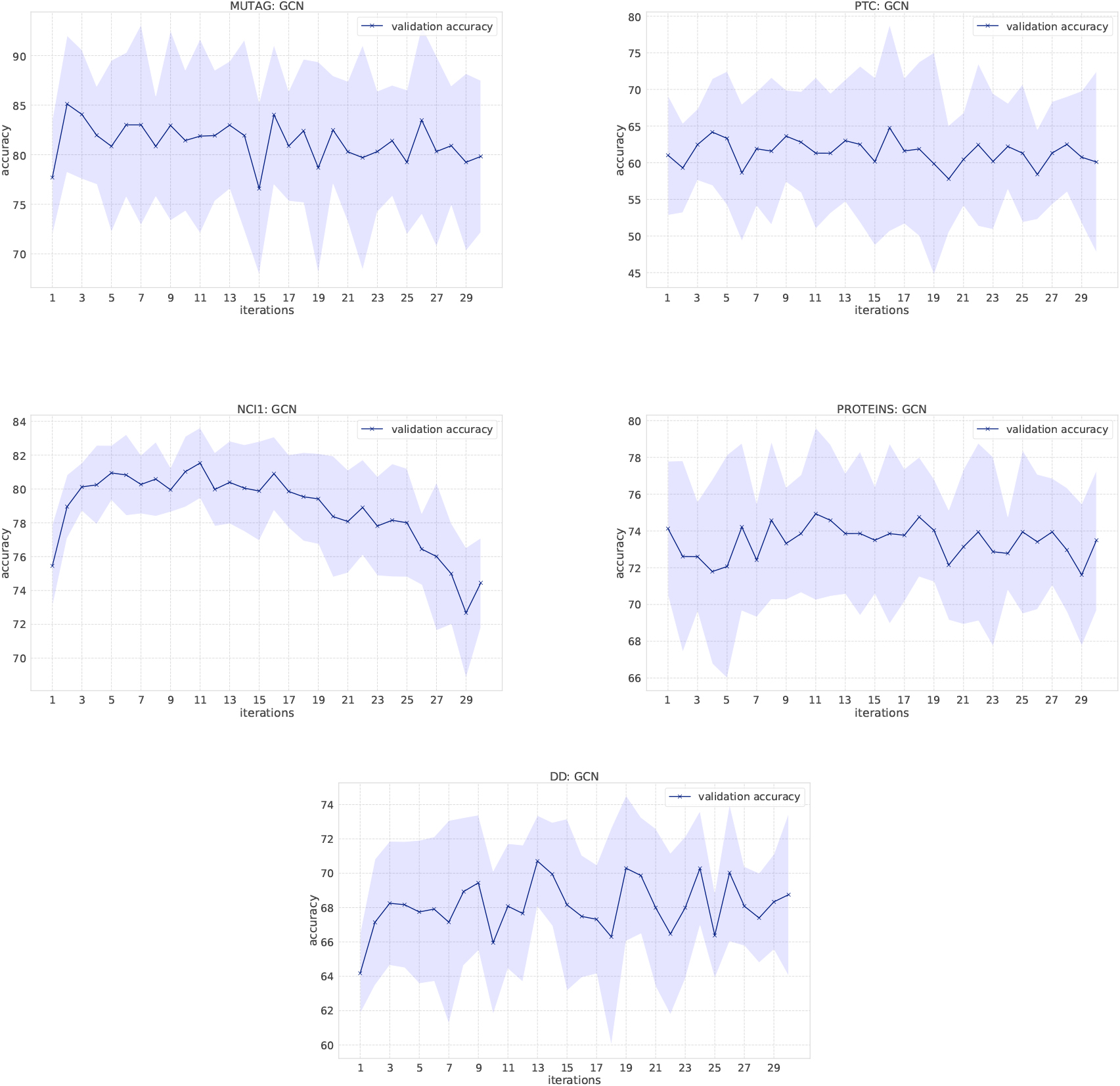
Figure 2.
Classification results of GINs on the bio-informatics dataset.
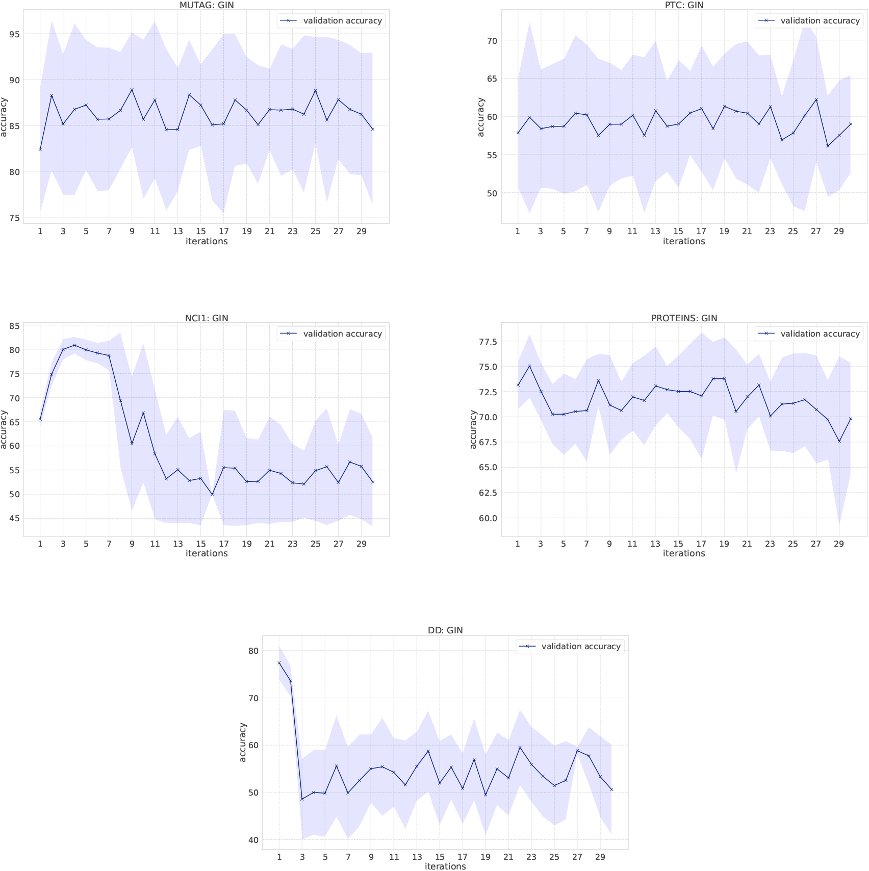
Figure 3.
Classification results on social network datasets.

Effects of the number of message passing iteration. Figures 1, 2, and 3 are classification results of GCNs and GINs when the amount of message passing increases, which investigates the impact of larger subgraph structures on its predictive performance. As the number of iterations increases, GCNs fail to appropriately learn representation of graphs in NCI1 and REDDIT-BINARY, and GINs fail in NCI1, PROTEINS, DD, REDDIT-BINARY, and IMDB-BINARY. One reason for this phenomenon is that GINs have more parameters than GCNs, so it is more difficult to effectively learn representation of node features as it is more affected by the previous ill-learned node features. However, as Tables 2 and 3 show, GINs are more powerful at learning representation of graphs on various datasets and also comparable to the WL kernel when such hyperparameters are properly tuned.
Figure 4.
Classification results of the WL kernel on Bio-informatics datasets.
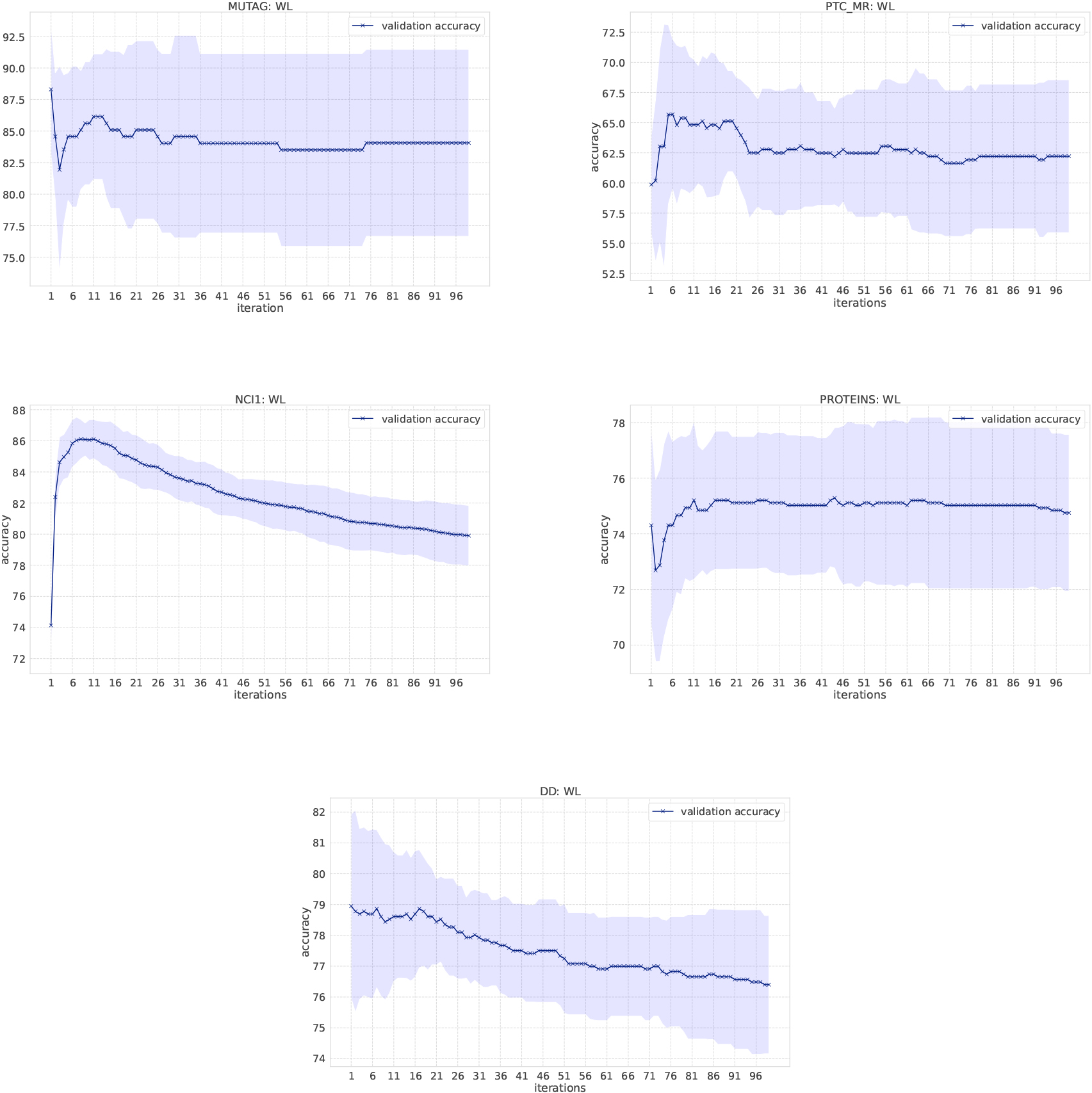
Figure 5.
Classification results on social network datasets.
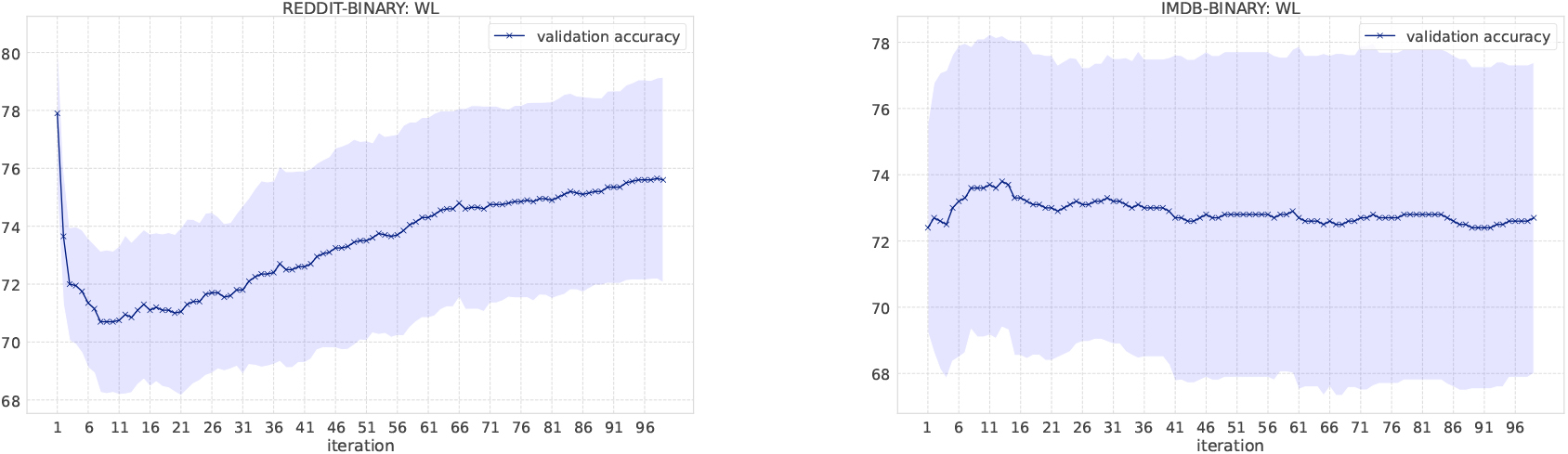
In the WL kernel, it is easy to compute the kernel even if the number of message passing iterations increases. Figure 4 shows the classification accuracy as the number of iterations increases. We have increased the number of iterations in the WL kernel up to 100. In the MUTAG dataset, labels obtained from the WL scheme become unique when iterations reach to 13, which means no more information gains. Small fluctuations of the resulting accuracy comes from the loop structure in graphs. Overall, the accuracy score is not largely affected by the number of iterations in the WL kernel, except for NCI1 and DD. One possible reason for such deteriorating accuracy in NCI1 and DD is that they have more node labels than other datasets and it becomes difficult to discriminate graphs as the number of iteration increases. Various node labels contribute to the occurrence of multiple types of unique subgraphs. Since graph kernels fundamentally measure the similarity between graphs based on subgraph matching, the kernel value gets smaller if there are many unique subgraphs. In the case of NCI1 and DD, when the number of iterations increases, more and more unique subgraphs appear, and the additional contribution to kernel values becomes smaller and smaller, resulting in the difficulty of discrimination. An interesting observation is that the accuracy on the REDDIT-BINARY dataset increases when the number of iterations increases, although the highest accuracy is at the first iteration.
Figure 6.
Accuracy and loss on MUTAG dataset.
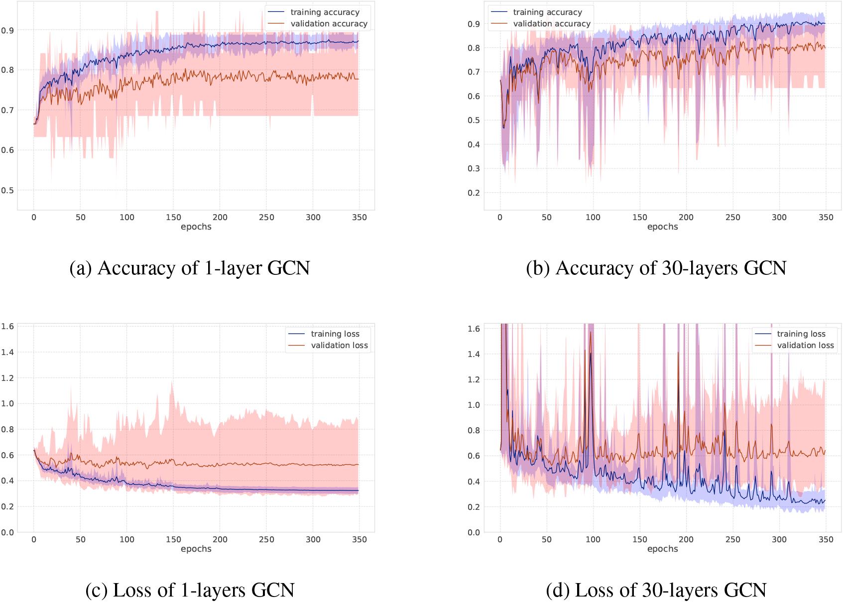
Figure 7.
Accuracy and loss on NCI1 dataset.
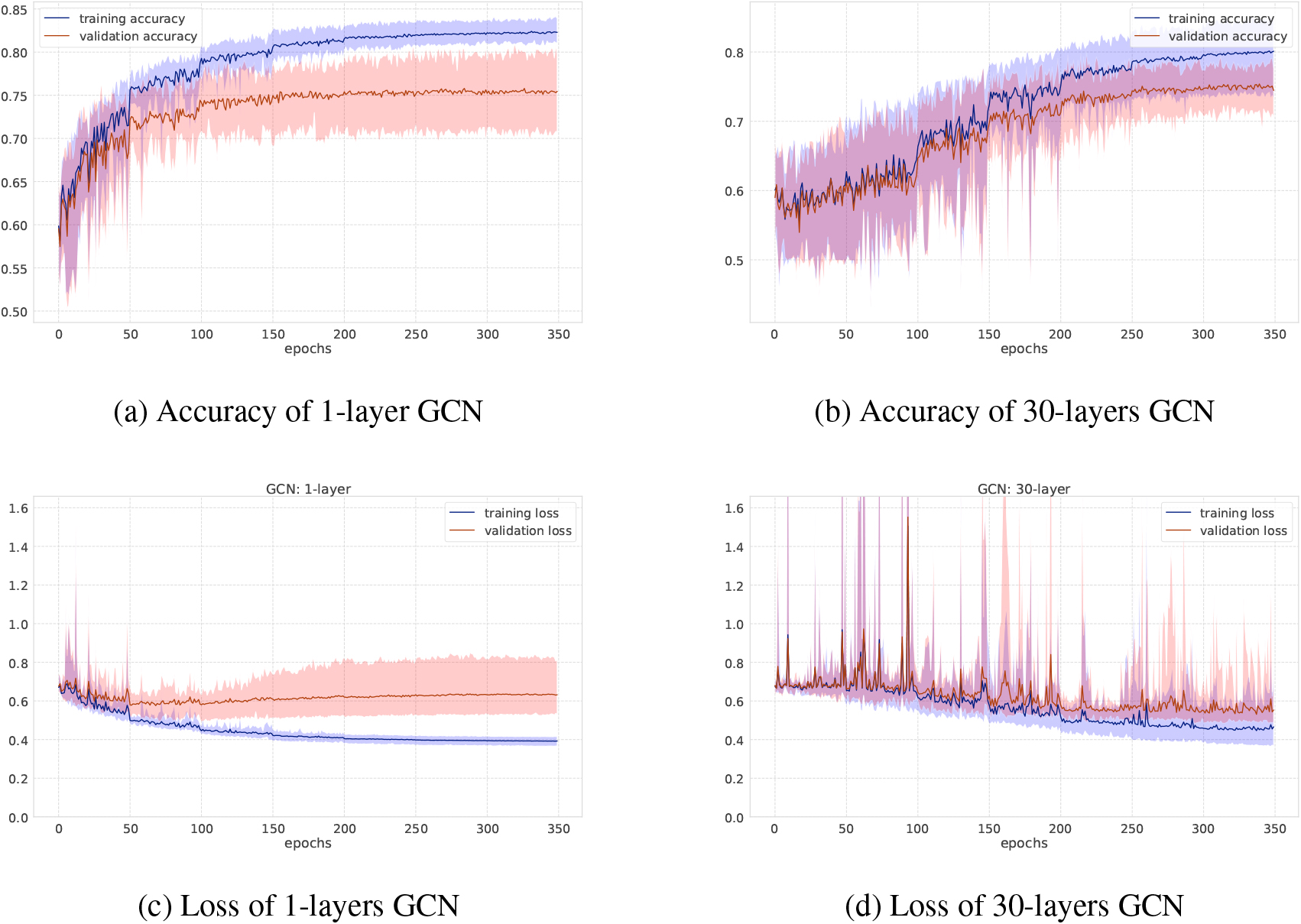
As for GCNs and GINs, Figs 6 and 7 show the training-validation loss and accuracy via 10-fold cross-validation per epoch on the MUTAG and NCI1 datasets. In each figure, left and right plots represent the training log of GCNs under the setting of the number of iterations 1 or 30, respectively. When the number of graph convolutional layers is one, the loss and accuracy of training-validation sets are rather smooth compared to the case where the number of graph convolutional layers is 30. After training after 350 epochs, the standard deviation of the training-validation loss and accuracy fluctuates greatly, although the final accuracy score is almost the same, at around 70 percent. This shows the difficulty of learning for a larger number of iterations where there are more trainable parameters as well. Figure 3 shows results on the social networks datasets. In GCNs, the accuracy does not change so much compared to GINs. All graphs on social network datasets have the same node labels, and GCNs may be easier to learn representation of node features, while GINs can get the best accuracy at the first or second steps.
Figure 8.
An example of transition of node features on MUTAG dataset. Each curve represents the averaged node feature value in a graph at each iteration step.
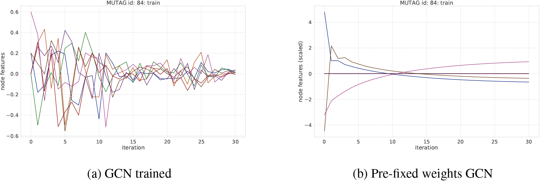
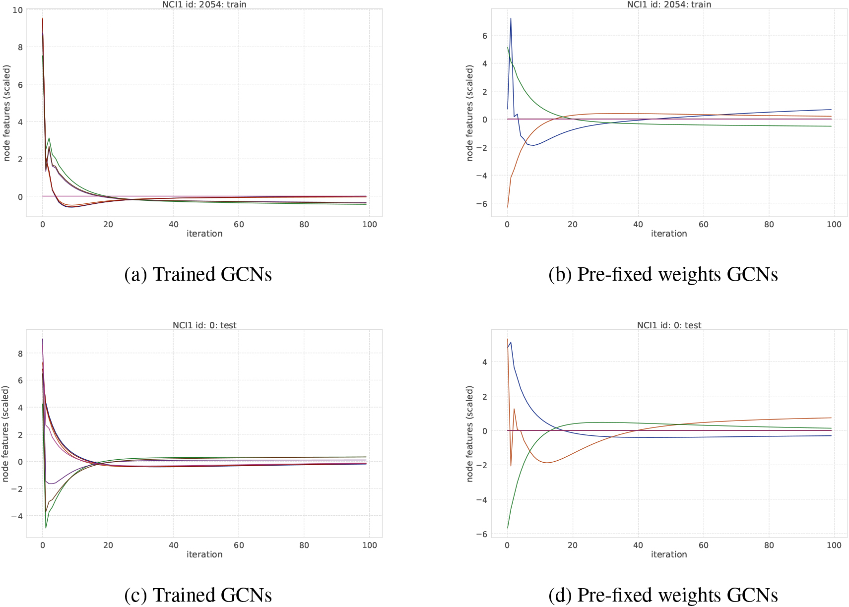
Transitions of node features over message passing iteration. To investigate how the number of message passing iterations affects the learning and how node features change through iteration, we plot the transition of node features shown in Figs 8 and 9. Figure 9 shows that node features in GCNs is likely to converge to a certain value on the NCI1 dataset, where over-smoothing is observed. Here, the size of features may be relevant to this phenomenon; that is, when the number of trainable parameters increases in graph convolutional layers, it is more difficult to learn the node features appropriately. As we can see in the MUTAG dataset in Fig. 8, when the weights are properly trained, even though the transition of node features tends to become small, the classification performance does not change.
Table 4
RMSE of holdout validation (training 70% test 30%). “
| Method | Dataset | |||||
| ESOL | Free solv | Lipophilicity | ||||
| 0-SVR | 1 | .127 | 1 | .951 | 1 | .019 |
| WL | 0 | .7686 | 1 | .112 | 0 | .6074 |
| Pre-fixed GCN SVR | 1 | .534 | 3 | .756 | 1 | .169 |
| 1-2 layers GCN | 0 | .8675 | 0 | .941334 | 0 | .688086 |
| 2 layers GCN | 1 | .270 | 1 | .3029752 | 0 | .8087 |
| 2 layers GIN | 0 | .8165 | 1 | .438 | 0 | .8118 |
| 30 layers GCN | 1 | .016 | 1 | .4068 | 1 | .219 |
| 30 layers GIN | – | 14 | .45463 | – | ||
Figure 9.
An example of transition of node features on NCI1 dataset. Each curve represents the averaged node feature value in a graph at each iteration step.
3.2.2Regression
Regression performance of each method. In addition to the classification task, we investigated the regression performance of WL kernels and GCNs. Results are shown in Table 4. In the table, 0-SVR is the linear kernel computed from the sum of initial node features across nodes, which is similar to the Vertex Histogram kernel. In chemo informatics datasets, graph features are often used as fingerprints (subgraphs in molecules) such as extended-connectivity fingerprints (ECFPs) [25] to deal with larger datasets. We chose smaller datasets for regression because ECFPs have a problem of bit collision, where fingerprints have duplication of subgraph structure in vectors. In the WL kernel, atomic numbers are directly used as node labels. The WL kernel shows the best result (the smallest RMSE) in ESOL and lipophilicity. GCNs and GINs are inferior to the WL kernel for the two datasets, while GCNs show the best score in FreeSolv using node features from two convolutional layers with their training.
Figure 10.
Regression results of SVR using node features learned from GCNs. Left plots show SVR results using features produced from each GCNs layer and right plots show SVR results using concatenating features.
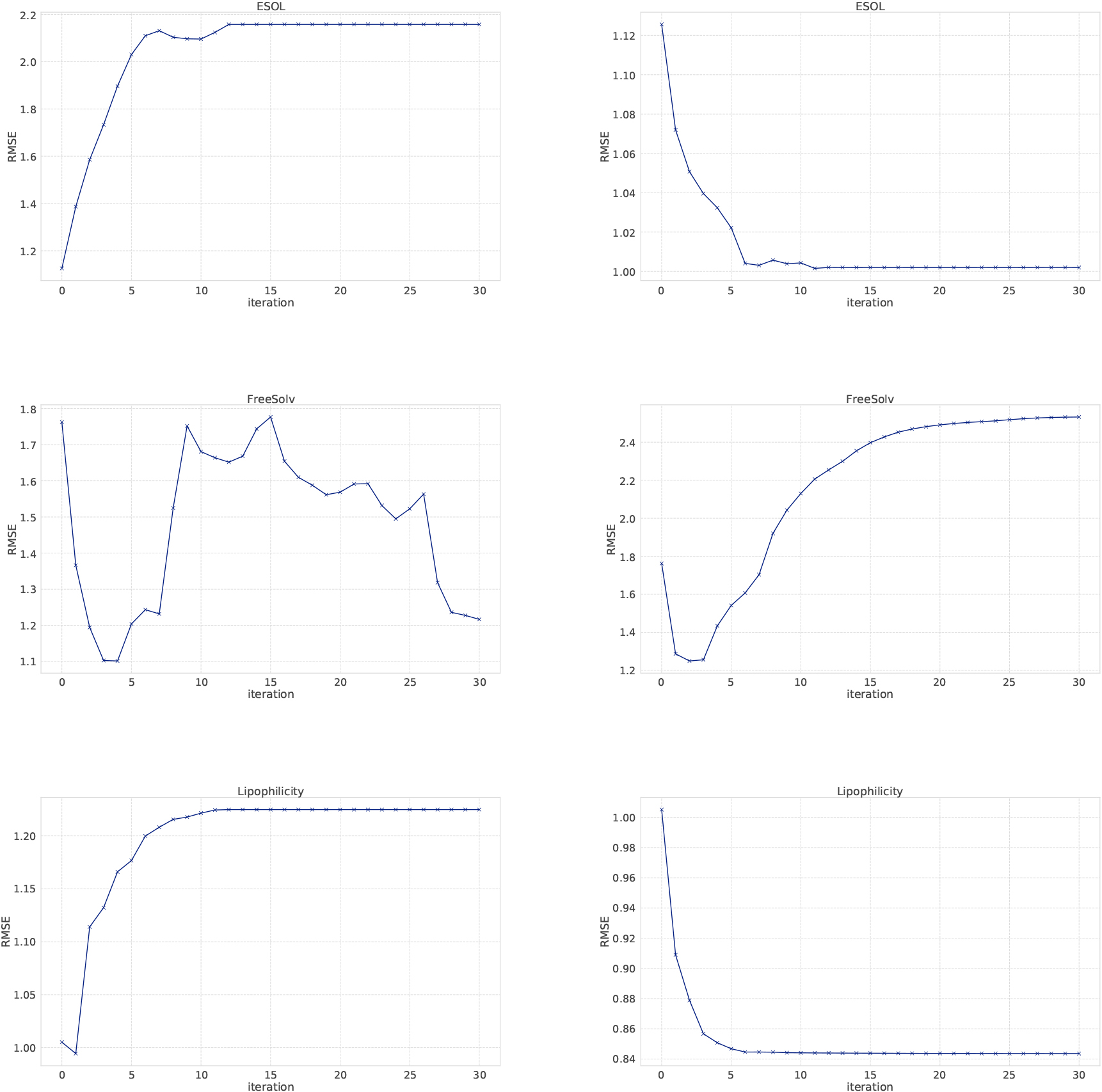
Effects of the number of message passing iteration. To investigate the impact of message passing iteration in the regression task, we plot RMSE results of SVR with node features learned from GCNs in Fig. 10. In the plots, the x-axis (iteration) means the number of message passing (graph convectional layers). In the left plots, the output of node features from each GCNs layer is used in SVR, and in the right plots, concatenated node features from GCNs are used in SVR. In ESOL and Lipophilicyty, an increase in the amount of message passing does not contribute to its predictive performance, while in FreeSolv it makes some contribution to the predictive performance. Concatenating graph features from each layers can be an effective choice when using a large number of iterations. In addition, the place where features from each GCNs layer become a plateau can provide good features. In FreeSolv, the score of GCNs with SVR fluctuates, and concatenating graph features gets the best score, at around five iterations. However, SVR is still effective and, with a little hyperparameter tuning, can learn the model with high predictive performance. The result of the RMSE of GCNs shows that increasing the number of message passing does not contribute to its predictive performance. Especially in GINs, the performance deteriorates, or learning is too unstable to train the model properly. This phenomenon often occurs, as shown in the classification section. However, as can be seen in Fig. 10, node features obtained from each layer in trained GCNs seem to be informative for SVR prediction on ESOL and lipophilicity datasets when concatenating these features. In contrast, the resulting RMSE of FreeSolv shows that calculated node features are likely to include noise because the performance of SVR decreases when they are concatenated. Therefore, as one of the options to circumvent the over-smoothing problem, we recommend empirically checking whether the iteration affects over-smoothing in SVR with node features learned from GCNs.
4.Conclusion
In this paper, we have investigated the effect of iterations of GCNs layers. In the WL kernel (which is the state-of-the-art graph kernel and shares the iteration process with GNNs to incorporate graph topological information), it usually maintains the good performance for large number of iterations in both classification and regression tasks. This may be because the WL kernel implicitly constructs a feature vector and addition of iteration means the concatenation, not the summation, of features. Since the large number of iterations means that the corresponding method tries to capture larger subgraphs, it can become insignificant if only local graph information is relevant. In GNN models such GCNs and GINs, by contrast, the number of iterations is largely affected because there are more and more trainable parameters and it is often difficult to learn them properly. Another reason could be that since node features can include noise, message passing iteration contributes to accumulate noise, resulting in worsening the performance of even the WL kernel. Since the predictive power of GCNs and GINs is comparable to that of the WL graph kernel, GNNs with mini-batch training can be an effective choice on larger dataset, as it is much more efficient than the WL kernel that requires the computation of the full kernel matrix. In our future work, we will investigate other methods such as attention-based graph neural networks.
Acknowledgments
This work was supported by JST, CREST Grant Number JPMJCR22D3, Japan, and JSPS KAKENHI Grant Number JP21H03503.
References
[1] | W.L. Hamilton, R. Ying and J. Leskovec, Inductive Representation Learning on Large Graphs, in: NIPS, (2017) . |
[2] | K. Xu, W. Hu, J. Leskovec and S. Jegelka, How Powerful are Graph Neural Networks? in: International Conference on Learning Representations, (2019) . https://openreview.net/forum?id=ryGs6iA5Km. |
[3] | P. Veličković, G. Cucurull, A. Casanova, A. Romero, P. Lió and Y. Bengio, Graph Attention Networks, in: International Conference on Learning Representations, (2018) . https://openreview.net/forum?id=rJXMpikCZ. |
[4] | J. Gilmer, S.S. Schoenholz, P.F. Riley, O. Vinyals and G.E. Dahl, Neural Message Passing for Quantum Chemistry, in: Proceedings of the 34th International Conference on Machine Learning – Volume 70, ICML’17, JMLR.org, (2017) , pp. 1263–1272. |
[5] | D. Bo, X. Wang, C. Shi and H. Shen, Beyond Low-frequency Information in Graph Convolutional Networks, arXiv, (2021) . doi: 10.48550/ARXIV.2101.00797. https://arxiv.org/abs/2101.00797. |
[6] | K. Borgwardt, E. Ghisu, F. Llinares-López, L. O’Bray and B. Rieck, Graph Kernels: State-of-the-Art and Future Challenges, Foundations and Trends® in Machine Learning 13: (5–6) ((2020) ), 531–712. doi: 10.1561/2200000076. |
[7] | H. Kashima, K. Tsuda and A. Inokuchi, Marginalized Kernels between Labeled Graphs, in: Proceedings of the Twentieth International Conference on International Conference on Machine Learning, ICML’03, AAAI Press, (2003) , pp. 321–328. ISBN 1577351894. |
[8] | M. Sugiyama and K. Borgwardt, Halting in Random Walk Kernels, in: Advances in Neural Information Processing Systems, Vol. 28, C. Cortes, N. Lawrence, D. Lee, M. Sugiyama and R. Garnett, eds, Curran Associates, Inc., (2015) . https://proceedings.neurips.cc/paper/2015/file/31b3b31a1c2f8a370206f111127c0dbd-Paper.pdf. |
[9] | N. Shervashidze, P. Schweitzer, E.J. van Leeuwen, K. Mehlhorn and K.M. Borgwardt, Weisfeiler-Lehman Graph Kernels, Journal of Machine Learning Research 12: (77) ((2011) ), 2539–2561. http://jmlr.org/papers/v12/shervashidze11a.html. |
[10] | T.N. Kipf and M. Welling, Semi-Supervised Classification with Graph Convolutional Networks, in: International Conference on Learning Representations (ICLR), (2017) . |
[11] | F. Scarselli, M. Gori, A.C. Tsoi, M. Hagenbuchner and G. Monfardini, The Graph Neural Network Model, IEEE Transactions on Neural Networks 20: (1) ((2009) ), 61–80. doi: 10.1109/TNN.2008.2005605. |
[12] | S. Brody, U. Alon and E. Yahav, How Attentive are Graph Attention Networks? arXiv, (2021) . doi: 10.48550/ARXIV.2105.14491. |
[13] | D. Chen, Y. Lin, W. Li, P. Li, J. Zhou and X. Sun, Measuring and Relieving the Over-Smoothing Problem for Graph Neural Networks from the Topological View, Proceedings of the AAAI Conference on Artificial Intelligence 34: (4) ((2020) ), 3438–3445. doi: 10.1609/aaai.v34i04.5747. |
[14] | N. Pržulj, Biological network comparison using graphlet degree distribution, Vol. 23, (2007) , pp. e177–e183. ISSN 1367-4803. doi: 10.1093/bioinformatics/btl301. |
[15] | N. Shervashidze, S. Vishwanathan, T. Petri, K. Mehlhorn and K. Borgwardt, Efficient graphlet kernels for large graph comparison, in: Proceedings of the Twelth International Conference on Artificial Intelligence and Statistics, D. van Dyk and M. Welling, eds, Proceedings of Machine Learning Research, Vol. 5, PMLR, Hilton Clearwater Beach Resort, Clearwater Beach, Florida USA, (2009) , pp. 488–495. https://proceedings.mlr.press/v5/shervashidze09a.html. |
[16] | K. Kersting, N.M. Kriege, C. Morris, P. Mutzel and M. Neumann, Benchmark Data Sets for Graph Kernels, (2016) , http://graphkernels.cs.tu-dortmund.de. |
[17] | Z. Wu, B. Ramsundar, E. Feinberg, J. Gomes, C. Geniesse, A.S. Pappu, K. Leswing and V. Pande, MoleculeNet: a benchmark for molecular machine learning, Chem. Sci. 9: ((2018) ), 513–530. doi: 10.1039/C7SC02664A. |
[18] | G. Siglidis, G. Nikolentzos, S. Limnios, C. Giatsidis, K. Skianis and M. Vazirgiannis, GraKeL: A Graph Kernel Library in Python, Journal of Machine Learning Research 21: (54) ((2020) ), 1–5. |
[19] | M. Wang, D. Zheng, Z. Ye, Q. Gan, M. Li, X. Song, J. Zhou, C. Ma, L. Yu, Y. Gai, T. Xiao, T. He, G. Karypis, J. Li and Z. Zhang, Deep Graph Library: A Graph-Centric, Highly-Performant Package for Graph Neural Networks, arXiv preprint arXiv:1909.01315, (2019) . |
[20] | M. Li, J. Zhou, J. Hu, W. Fan, Y. Zhang, Y. Gu and G. Karypis, DGL-LifeSci: An Open-Source Toolkit for Deep Learning on Graphs in Life Science, ACS Omega ((2021) ). |
[21] | A. Paszke, S. Gross, F. Massa, A. Lerer, J. Bradbury, G. Chanan, T. Killeen, Z. Lin, N. Gimelshein, L. Antiga, A. Desmaison, A. Kopf, E. Yang, Z. DeVito, M. Raison, A. Tejani, S. Chilamkurthy, B. Steiner, L. Fang, J. Bai and S. Chintala, PyTorch: An Imperative Style, High-Performance Deep Learning Library, in: Advances in Neural Information Processing Systems 32, Curran Associates, Inc., (2019) , pp. 8024–8035. http://papers.neurips.cc/paper/9015-pytorch-an-imperative-style-high-performance-deep-learning-library.pdf. |
[22] | J.H. Xifeng Yan, gSpan: Graph-Based Substructure Pattern Mining, International Conference on Data Mining ((2002) ), pp. 721–724. doi: 10.1109/ICDM.2002.1184038. |
[23] | F. Pedregosa, G. Varoquaux, A. Gramfort, V. Michel, B. Thirion, O. Grisel, M. Blondel, P. Prettenhofer, R. Weiss, V. Dubourg, J. Vanderplas, A. Passos, D. Cournapeau, M. Brucher, M. Perrot and E. Duchesnay, Scikit-learn: Machine Learning in Python, Journal of Machine Learning Research 12: ((2011) ), 2825–2830. |
[24] | D.P. Kingma and J. Ba, Adam: A Method for Stochastic Optimization, arXiv, (2014) . doi: 10.48550/ARXIV.1412.6980. |
[25] | D. Rogers and M. Hahn, Extended-Connectivity Fingerprints, Journal of Chemical Information and Modeling 50: (5) ((2010) ), 742–754. doi: 10.1021/ci100050t. |
[26] | D. Chen, Y. Lin, W. Li, P. Li, J. Zhou and X. Sun, Measuring and Relieving the Over-smoothing Problem for Graph Neural Networks from the Topological View, arXiv, (2019) . doi: 10.48550/ARXIV.1909.03211. |
[27] | C. Morris, M. Ritzert, M. Fey, W.L. Hamilton, J.E. Lenssen, G. Rattan and M. Grohe, Weisfeiler and Leman Go Neural: Higher-Order Graph Neural Networks, in: Proceedings of the Thirty-Third AAAI Conference on Artificial Intelligence and Thirty-First Innovative Applications of Artificial Intelligence Conference and Ninth AAAI Symposium on Educational Advances in Artificial Intelligence, AAAI’19/IAAI’19/EAAI’19, AAAI Press, (2019) . ISBN 978-1-57735-809-1. doi: 10.1609/aaai.v33i01.33014602. |
[28] | C. Morris, N.M. Kriege, F. Bause, K. Kersting, P. Mutzel and M. Neumann, TUDataset: A collection of benchmark datasets for learning with graphs, in: ICML 2020 Workshop on Graph Representation Learning and Beyond (GRL+ 2020), (2020) . www.graphlearning.io. |

