
sKAdam: An improved scalar extension of KAdam for function optimization
Abstract
This paper presents an improved extension of the previous algorithm of the authors called KAdam that was proposed as a combination of a first-order gradient-based optimizer of stochastic functions, known as the Adam algorithm and the Kalman filter. In the extension presented here, it is proposed to filter each parameter of the objective function using a 1-D Kalman filter; this allows us to switch from matrix and vector calculations to scalar operations. Moreover, it is reduced the impact of the measurement noise factor from the Kalman filter by using an exponential decay in function of the number of epochs for the training. Therefore in this paper, is introduced our proposed method sKAdam, a straightforward improvement over the original algorithm. This extension of KAdam presents a reduced execution time, a reduced computational complexity, and better accuracy as well as keep the properties from Adam of being well suited for problems with large datasets and/or parameters, non-stationary objectives, noisy and/or sparse gradients.
1.Introduction
In a previous work of the authors [2], the KAdam algorithm was introduced as a first-order method for stochastic function optimization. For the design of the KAdam algorithm, it was assumed that for each layer in a neural network there is an associated true state vector from a linear dynamic system, where, the predicted state estimated vector has the same dimension as the sum of the dimensions from the stacked weights and biases of its layer.
With the presentation of KAdam, it is confirmed that by using the Kalman filter [5] with Adam [6], the filter can add significant and relevant enough variations to the gradient (similar to the additive white noise randomly included to the gradient [7]) in order to find better solutions in the loss function. Furthermore, this version shows that it could be used as an initializer in on-line settings compared with: Momentum [9], RMSProp [11], and Adam [6].
However, even that KAdam presents a great performance in the carried out experiments, the time that takes to train a neural network is out of comparison with other gradient-based optimizers. The problem is that the size of the matrices from the Kalman filter depends on the number of neurons used per layer in the neural network architecture. Hence, if the number of neurons is increased, the dimension of the matrices directly affects the time that takes to compute the matrix inverse. Furthermore, the authors realized that when the loss is near to the neighborhood of the optimal minimum, KAdam starts to present a noisy behavior due to the fixed measurement noise considered for the Kalman filters. Thus, if the number of epochs needed to converge is increased, the algorithm present problems to reach lower values in the loss function.
In order to solve the identified problems, firstly, in the design of the new algorithm, it is proposed to use 1-D Kalman filters for each parameter from the loss function instead of using one Kalman filter per layer on the neural network. On the other hand, it was used an exponential decay over the measurement noise considered in the Kalman filters.
With these changes to the original algorithm, it is presented sKAdam our extension for KAdam using the scalar Kalman filter. Our method achieves to reduce the time taken to optimize a function and also improve the algorithmic complexity.
This paper is organized as follows, in the next section a quick description of the gradient descent algorithm is made, their variants and some of their most popular state-of-the-art optimizations. Then, in Section 3 a brief introduction to the Kalman filter and its implementation for a 1-D problem is provided. After that, in Section 4 the sKAdam algorithm is presented. Subsequently, in Section 5 the performance of our proposal is compared with other gradient-based optimizers for different classification and regression benchmark problems. Finally, Section 6 is devoted to conclusions and future work.
2.Gradient descent
Gradient descent is a first-order method to perform stochastic functions optimization.
Let
The gradient descent algorithm in neural networks is one of the most popular techniques used to update the parameters (weights and biases) of the model, using the loss function as the objective function to optimize.
2.1Variants
The gradient descent algorithm has three main variants: Stochastic gradient descent (SGD), Batch gradient descent (Batch GD a.k.a. Vanilla GD) and Mini-batch gradient descent (Mini-batch GD); which differs in the amount of data used to compute the gradient.
Stochastic gradient descent performs a parameters update for each pattern
(1)
Usually this variant is more accurate while it is updating the parameters, but it takes longer to finish the optimization because of the number of updates that the algorithm performs.
Batch gradient descent computes the gradient for all the patterns in the training-set, then it performs a parameters update using the average direction from all the gradients.
(2)
Compared to SGD this variant is faster when it is updating the parameters. However, this speed improvement directly affects the accuracy of the parameter updates.
Mini-batch gradient descent divides the training-set in mini-batches and performs a parameters update with each mini-batch.
(3)
This variant has the best from both worlds; it combines part of the accuracy from SGD and the speed improvement from Batch GD. Theoretically, there is an optimal mini-batch size where the performance and the computational complexity are balanced.
2.2Gradient-based optimizers
There are different methods designed in order to accelerate and improve the gradient descent algorithm and its variants. Each state-of-the-art method present its own strengths and weaknesses, see [10] for further details with a deeper overview.
From here, let
Momentum[9] introduces the idea of using a fraction
(4)
(5)
The momentum term drives the parameters into a relevant direction, accelerating the learning process and dampening oscillations on the parameters update. However, the same term could present a blind-rolling behaviour on the algorithm, because it keeps accumulating momentum from the previous update vectors.
AdaGrad[1] solved the blind-rolling behaviour by using adaptive learning rates for each parameter.
(6)
In Eq. (6),
One of the best features from AdaGrad is that it reduce the importance of tuning the learning rate manually. Nevertheless, this main advantage is also a problem at a certain point of the optimization because the learning rate start to shrink and eventually it will be infinitesimal, hence the algorithm will be no longer able to keep learning.
Adadelta[13] is an extension of AdaGrad, which solves the problem of the radically diminishing learning rates by restricting the accumulated past squared gradients to some fixed size window.
(7)
(8)
where, RMS stands for Root Mean Square. In Eq. (7), the numerator is used as an acceleration term by accumulating previous gradients similar to the momentum term, but with a fixed size window. The denominator is related to AdaGrad by saving the squared past gradient information, but with a fixed size window to ensure progress is made later in training.
RMSProp is an unpublished algorithm by Geoffrey Hinton that was reported in the Lecture 6 of his online course [11]. Moreover, this method was developed around the same time that Adadelta, and even with the same purpose of reducing the AdaGrad’s radically diminishing learning rates.
(9)
(10)
Similar to AdaGrad the RMSProp’s algorithm is storing the past squared gradients, but instead of keep accumulating them over the training, it is using an exponential moving average
Curiously, in the Adadelta’s method derivation in [13], it can be observed that before the second idea of its authors the update parameters rule is just like the update rule from RMSProp; but the authors of Adadelta considered an extra term to make a units correction over the parameters and not the gradient.
Adam[6] is one of the most popular and used optimizers in the training of neural networks. The method is described by its authors as a combinations from the advantages of AdaGrad and RMSProp.
(11)
(12)
(13)
(14)
(15)
Adam has the best from both worlds, the algorithm is using exponential moving averages over the past gradient (
3.Kalman filter
The Kalman filter [5] is a recursive state estimator for linear systems. First lets assume a dynamic linear system in the state space format:
(16)
where given the time-step
The true state vector
(17)
where,
Therefore, the Kalman filter provides estimates of some unknown variables given observed measurements over time. The estimation can be divided into a two-step process: prediction and update.
First, a predicted (a priori) state estimate
(18)
(19)
Then, for the update phase, the optimal kalman gain matrix
(20)
(21)
(22)
3.1Scalar Kalman filter
In Eqs (16) to (17) the true state, dynamical model, and measurements are described with vectors and matrices. On the other hand, if the problem described lies in 1-D vector space, then it is represented in terms of scalars and constants. Thus, the equations for the Kalman filter can be rewritten as follows:
(23)
(24)
(25)
(26)
(27)
where, the matrix operations are replaced with scalar operations and the matrix inverse is replaced with the scalar multiplicative inverse (reciprocal value).
4.sKAdam
In the design of the KAdam’s algorithm one Kalman filter for each layer of the neural network was used, i.e. assuming a neural network with
As can be seen in Eq. 20 there is an inverse matrix computed for the Kalman filter, then the algorithmic complexity is in function of the architecture for the neural network. Moreover, if this first version is used in on-line training settings the algorithm takes longer to finish the optimization compared with other gradient-based optimizers.
For sKAdam design, it is proposed to use one Kalman filter for each parameter of the loss function. Hence, the Eqs (23) to (27) can be used because now the problem lies in 1-D.
4.1Kalman filter parameters
Similar to the first version of KAdam, the variables
(28)
where
With these considerations, the Eqs (23) to (27) of the scalar Kalman filter for this particular implementation can be rewritten as follows:
(29)
(30)
(31)
(32)
(33)
4.2sKAdam algorithm
The equations for sKAdam use a
(34)
Then the equations for the first Eq. (11) and second Eq. (12) moments estimated from Adam now use the estimated gradient:
(35)
(36)
and the equations for the bias-corrected first moment estimate Eq. (13), the bias-corrected second moment estimate Eq. (14), and the parameters update rule Eq. (15), they remain the same as in the Adam algorithm.
In Algorithm 1 is shown the pseudocode for sKAdam.
sKAdam our new proposed an optimized extension of KAdam
5.Experiments
To empirically evaluate the performance of our method, different experiments werew carried out with popular benchmark classification and regression problems. In the experiments there is a comparison over the loss reduction in mini-batch and full-batch settings against other gradient-based optimizers, using feed-forward neural networks with fixed architectures (experimentally selected according each experiment) and the mean squared error (MSE) as the loss function.
In every experiment, all the models start the optimization with the same parameters (weights), which are randomly initialized. The settings for the hyper-parameters of the optimizers are the recommended by the authors of each algorithm, except for the learning-rate which is fixed here to the value of
Each experimental result and comparison is presented in two figures in order to the reader can clearly appreciate the dynamic of each algorithm because the lines that represent each algorithm behaviour overlap very often and they can occlude each other.
5.1MNIST database classification experiment
The popular classification problem for the hand written numbers. Originally the dataset consists of images of 28
Figure 1.
MNIST 2-D visualization using the t-SNE implementation from scikit-learn.
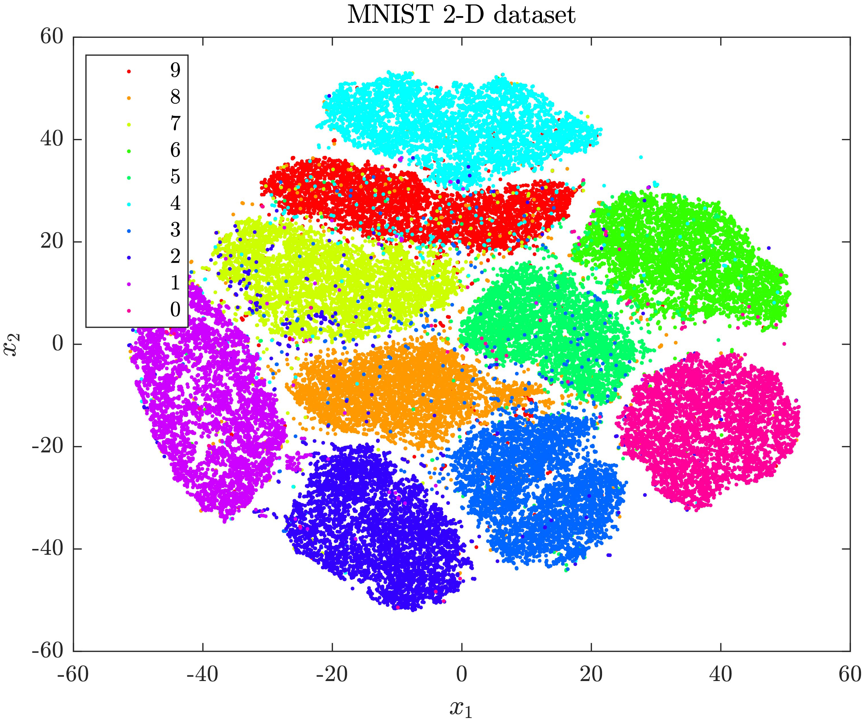
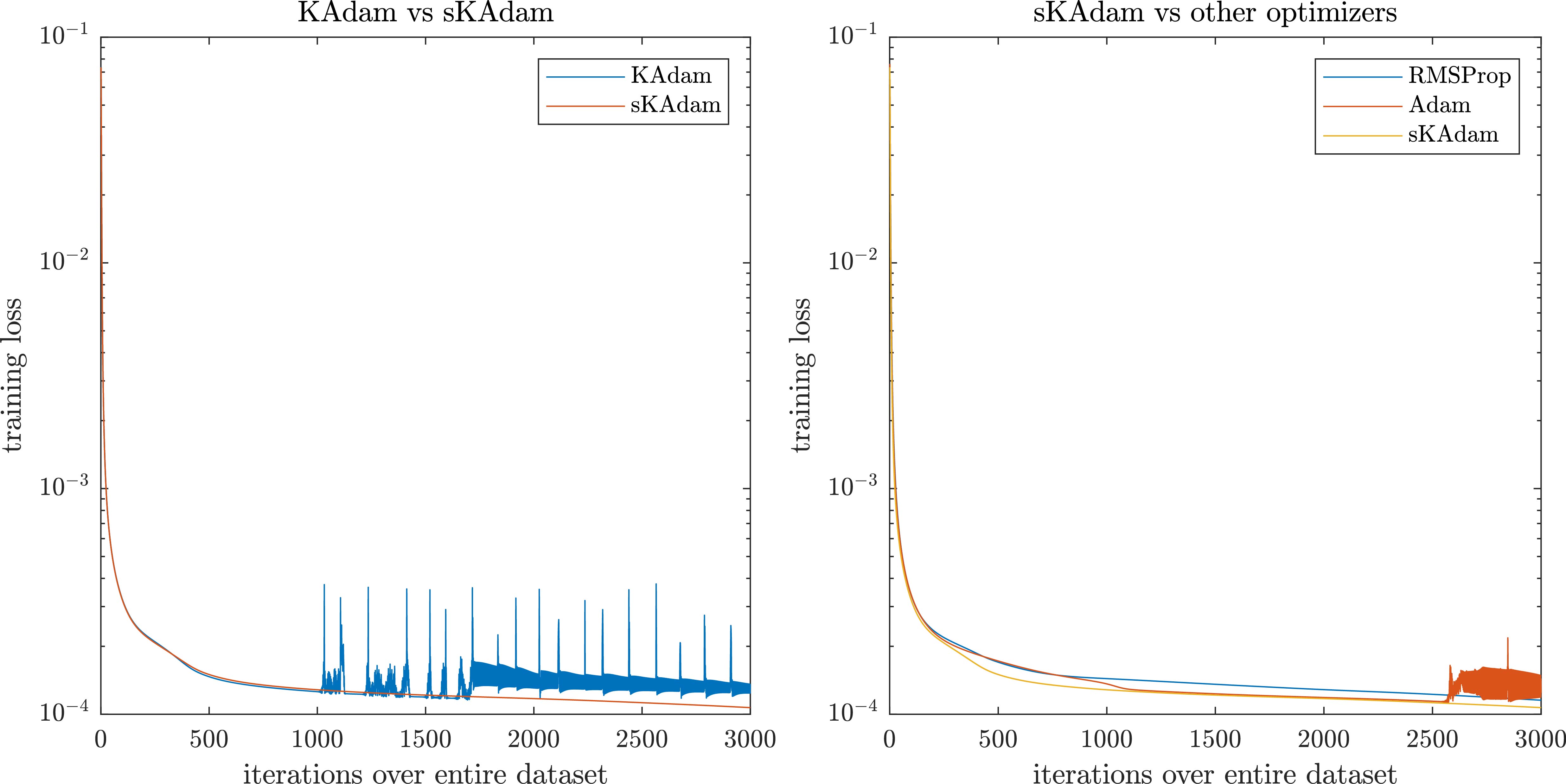
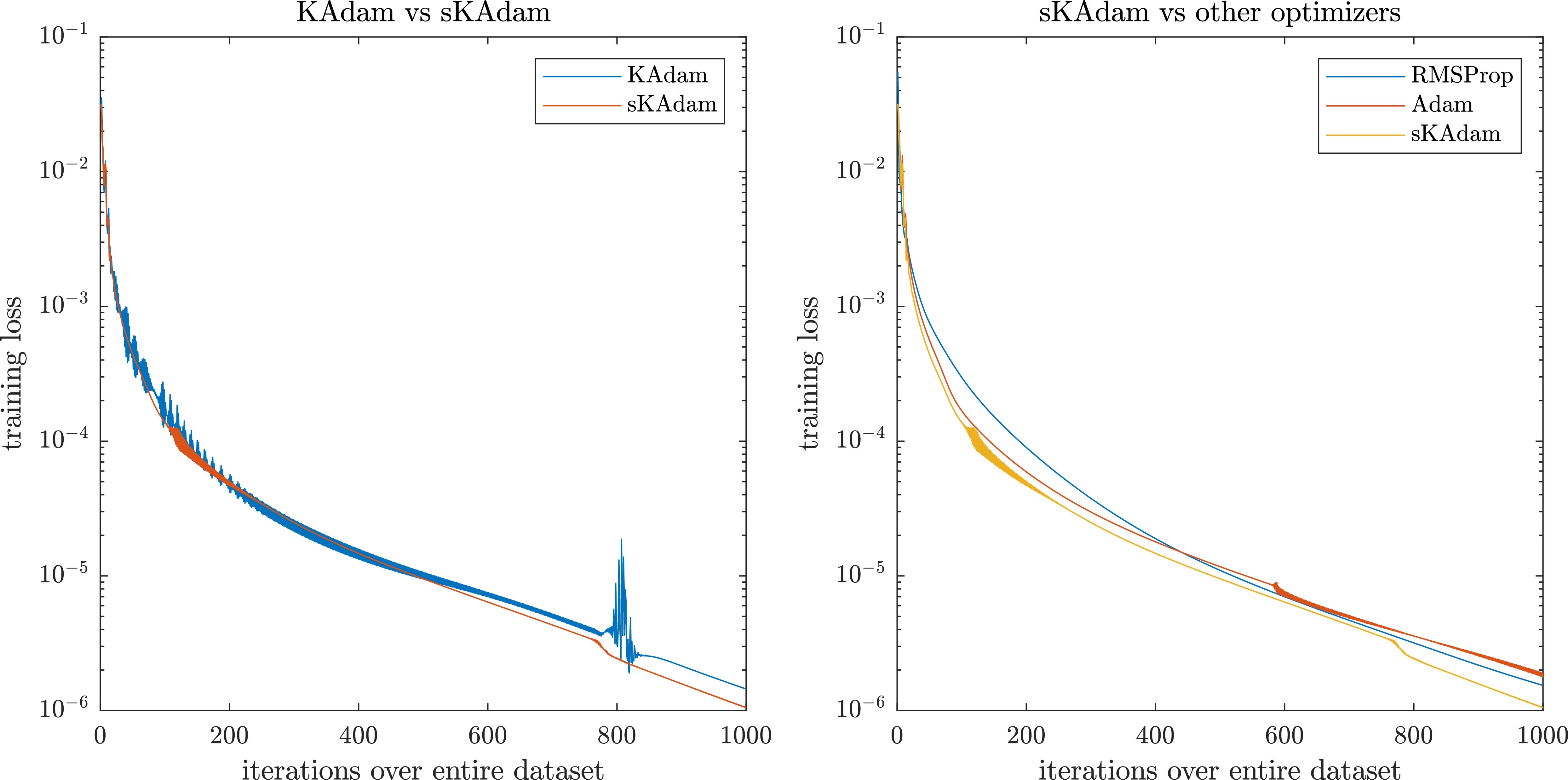
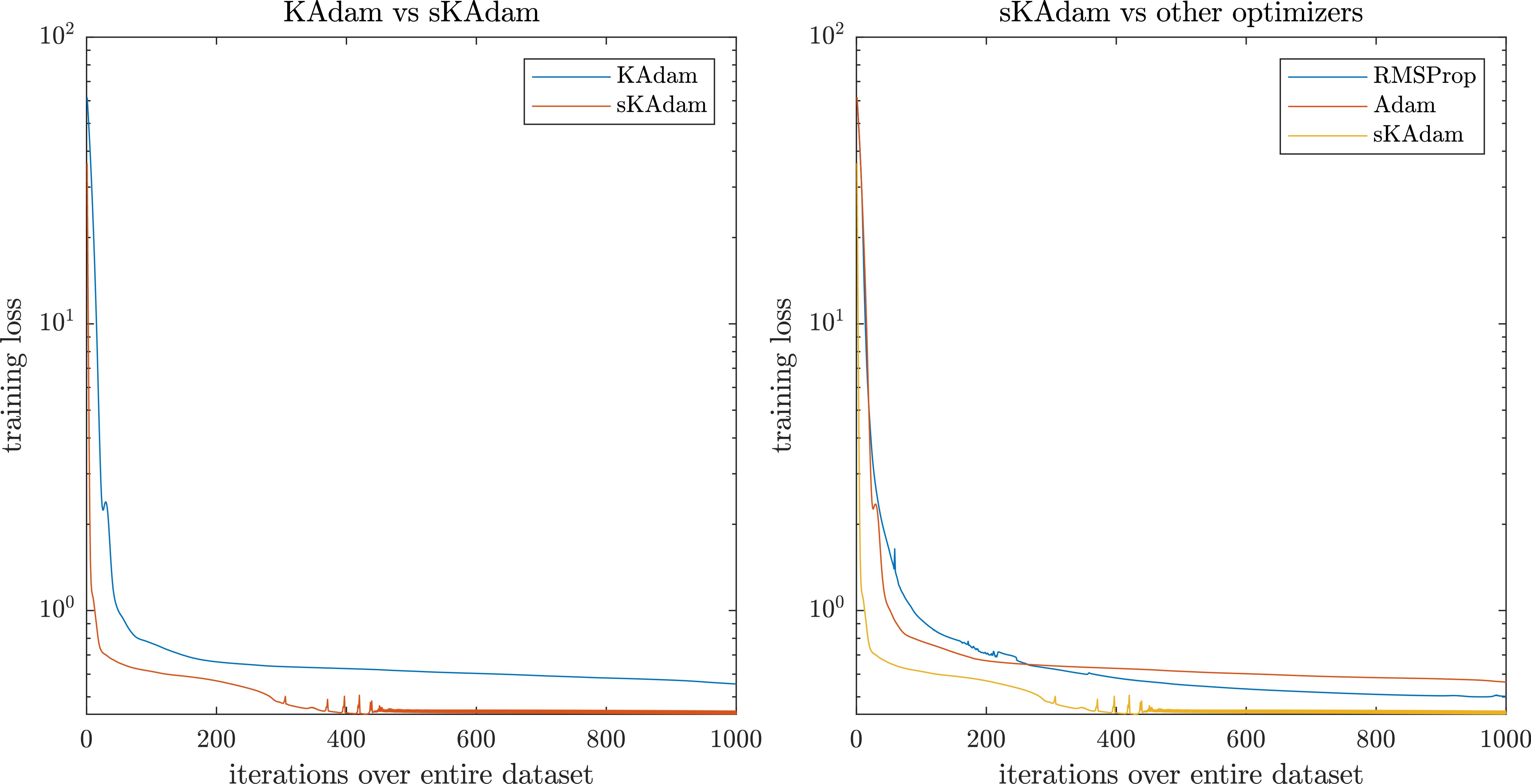
Figure 2.
MNIST experiment in mini-batch settings – comparison of the loss optimization over the trainings.
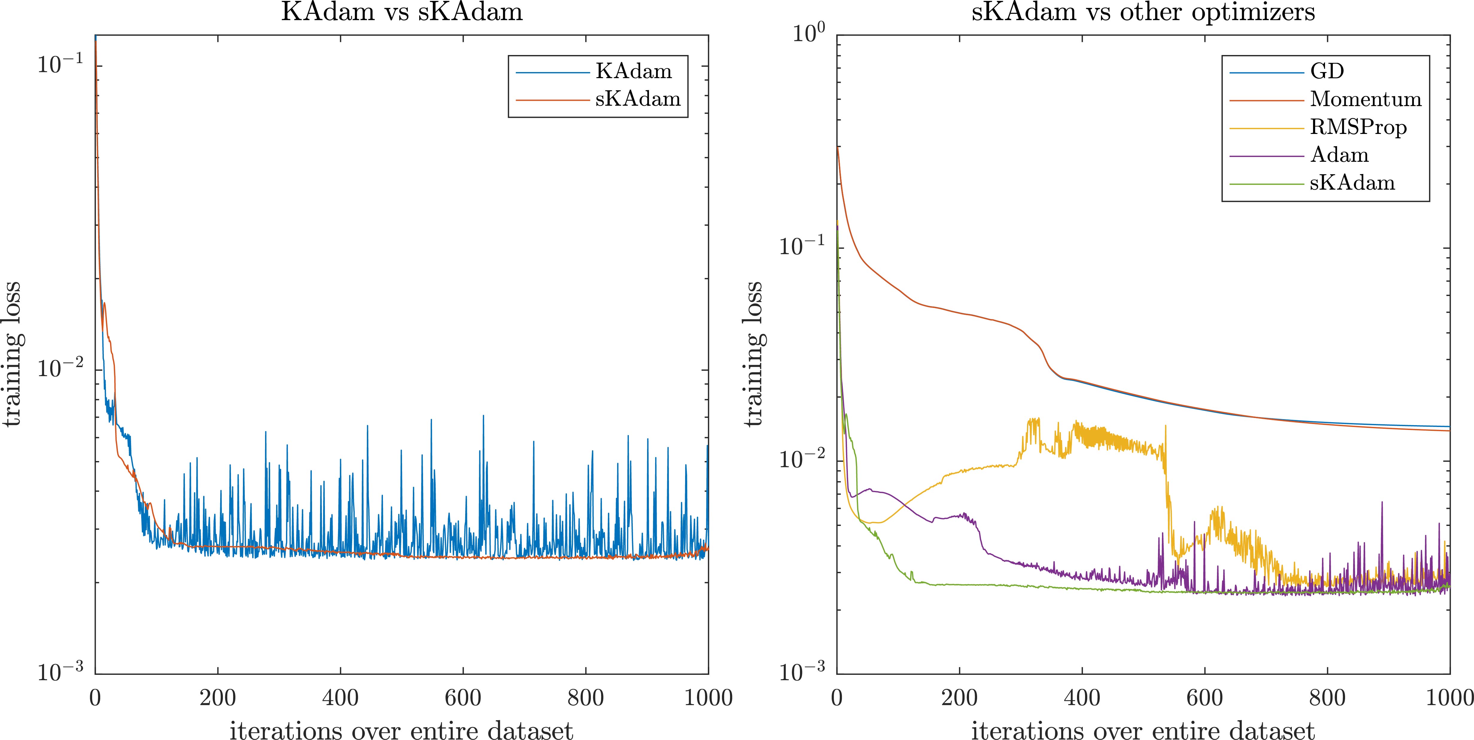
For the architectures of the neural networks were set to (10, 10) neurons, hyperbolic tangent and sigmoid as the activation functions respectively. All the algorithms performs the optimization with 60,000 patterns from the transformed dataset over 1,000 epochs.
As a first comparison, the training was run in mini-batch settings to test the improvement in the execution time that sKAdam reaches. Also, the performance in the optimization was tested and the loss reduction of our method was compared against GD, Momentum, RMSProp, Adam, and KAdam.
In Fig. 2 it can be observed the experiment in mini-batch settings. Here, on the left side, it can be seen that sKAdam presents the smoothest descent in comparison with the original KAdam’s algorithm. Furthermore, on the right side of the figure, it can be seen that sKAdam reaches an optimal value near to the epoch 120 and keeps closer to this optimal value until the end of the optimization. On the other hand, the other adaptive learning-rate methods reach similar results until the epoch 500 but with noisy behaviors, which can be undesirable in an on-line training setting where the adapted variables could have a physical interpretation and to present large variations in the values of the variables can represent a risk of damage to the system being controlled.
In a second comparison, the training was run in full-batch settings, where the authors already know that the execution time may not present a considerable difference with the original KAdam’s algorithm and the other optimizers.
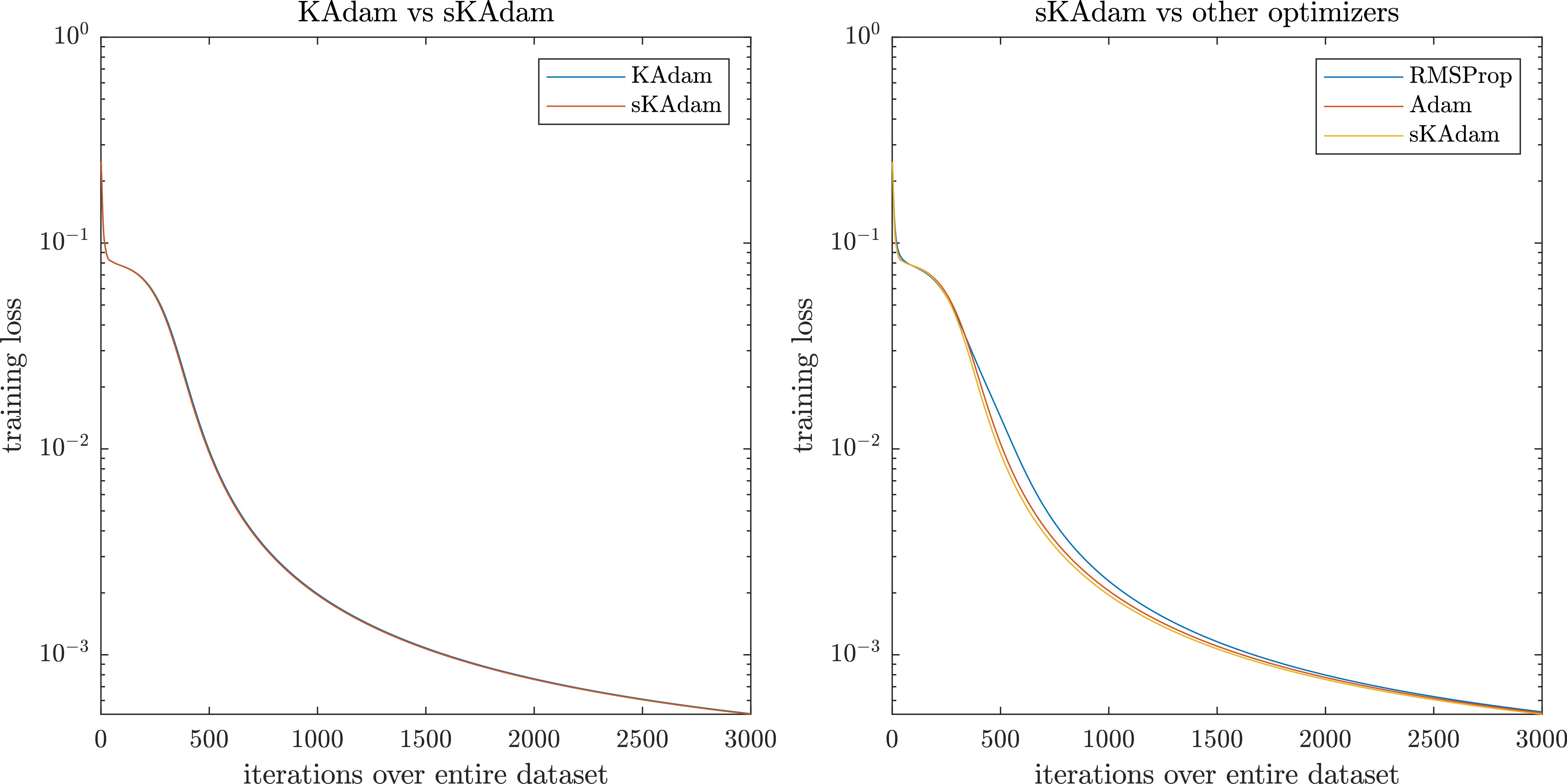
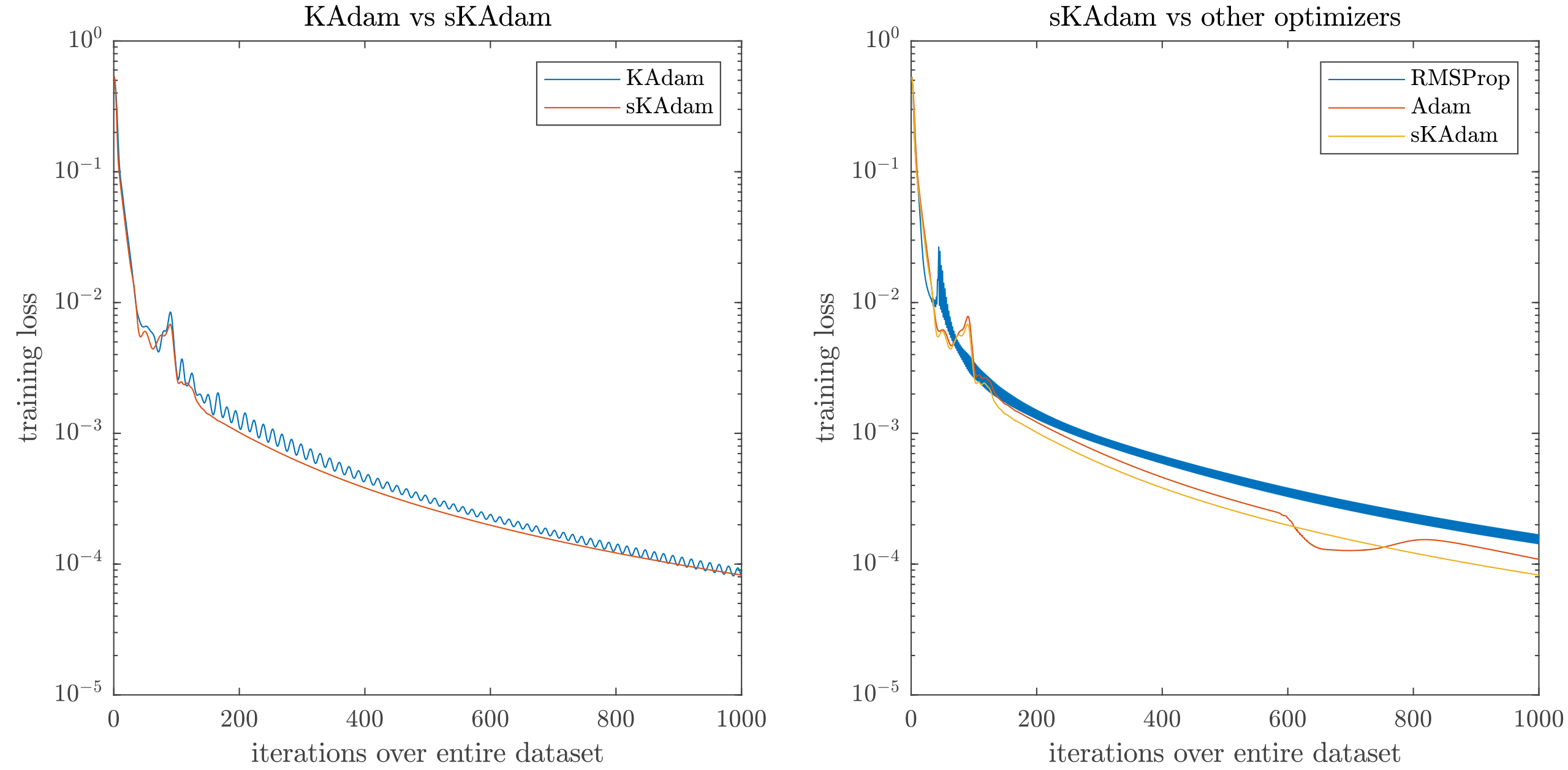
Figure 3.
MNIST experiment in full-batch settings – comparison of the loss optimization over the trainings.
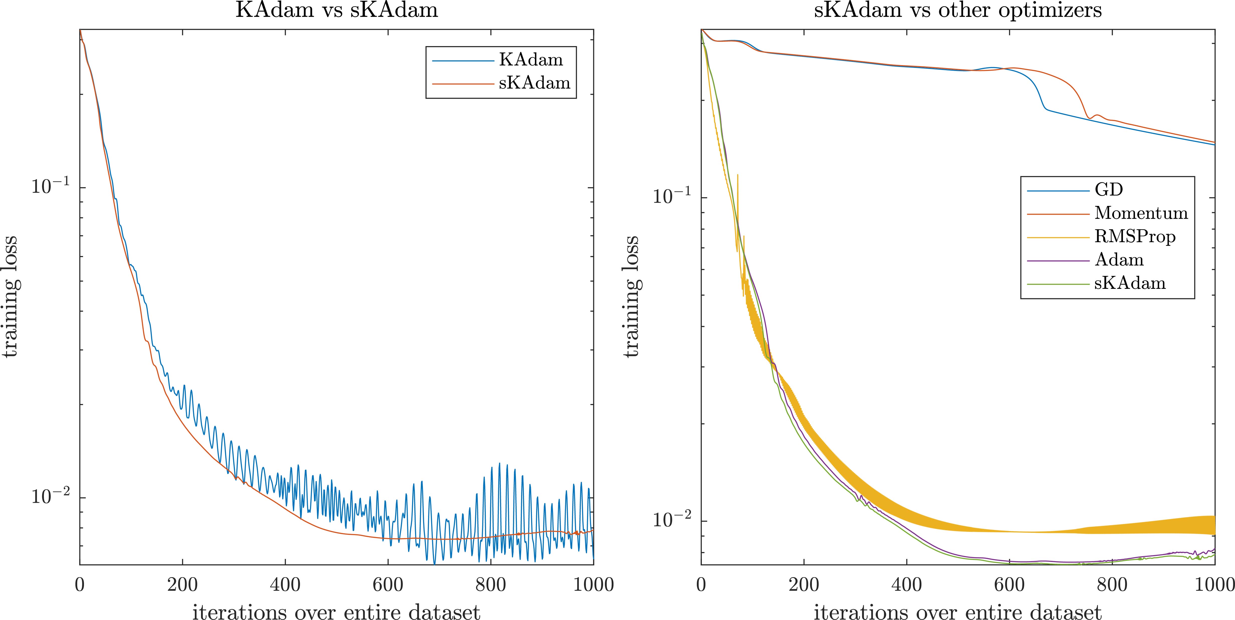
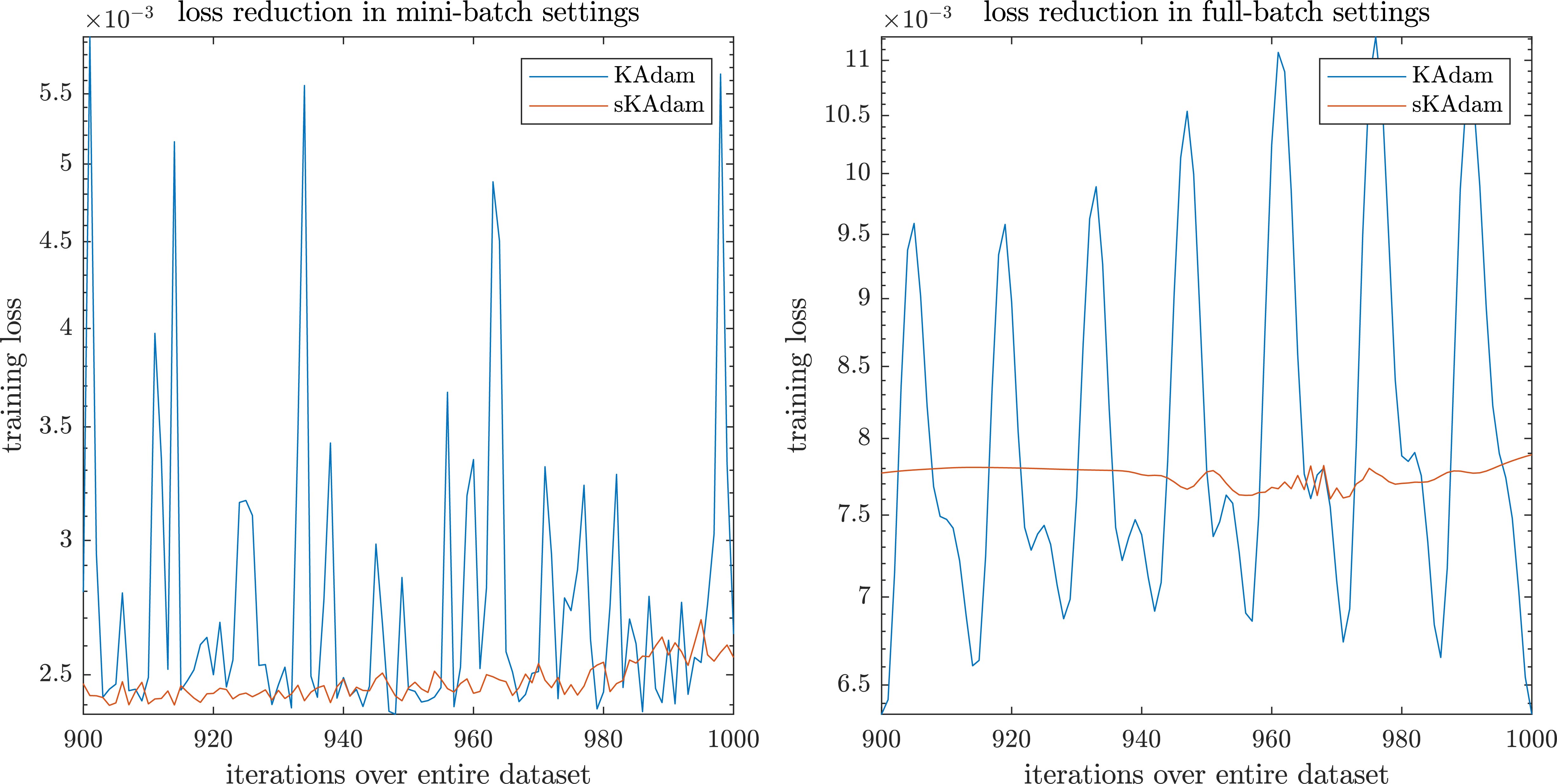
Figure 4.
MNIST experiment – last 100 epoch of the trainings.
This time, at the left side of Fig. 3 it can be seen that again sKAdam presents a smoother behavior compared with KAdam. However, on the right side, it can be observed that the adaptive learning-rate methods present similar results, and only RMSprop presents noisy behavior.
In Fig. 4 there is a close up to the dynamics of KAdam and sKAdam in the last 100 iterations of both mini-batch and full-batch trainings. Here, it is clear to see that even when KAdam and sKAdam are similar methods, they present completely different dynamics due to the noise measurement factor considered for each algorithm. As the authors previously mentioned, besides the problem of the execution time, there is another problem in KAdam related to the fixed noise measurement matrix. Which at the early stages of the optimization, this fixed matrix helps to reach new solutions with the estimated gradients as well as present a faster descent, but later in training it makes it harder to reach new solutions and also the converge of the algorithm present a noisy dynamic.
Nevertheless, as it can be observed the sKAdam method shows the importance of the exponential decay included to reduce the noise factor over the optimization.
Table 1 presents a summary of the results obtained over the optimization in both settings. Where it can be seen how even that KAdam and sKAdam are similar algorithms, they present a considerable difference in the execution time using mini-batch settings, which is a consequence of the matrix inverse computed in KAdam vs the simpler calculation of the scalar multiplicative inverse that sKAdam performs. In Table 1, the columns min. loss present the minimum value for the loss function found for each algorithm, the columns min
Table 1
MNIST – Comparison table
| Mini-batch | Full-batch | |||||
|---|---|---|---|---|---|---|
| Min. loss | Min | Time (s) | Min. loss | Min | Time (s) | |
| GD | 0.0145 | 9.4271e-04 | 130.13 | 0.1456 | 0.0027 | 212.22 |
| Momentum | 0.0139 | 9.5152e-04 | 137.27 | 0.1484 | 0.0023 | 220.97 |
| RMSProp | 0.0025 | 4.9094e-05 | 141.87 | 0.0091 | 0.0019 | 222.25 |
| Adam | 0.0023 | 3.5957e-05 | 143.90 | 0.0075 | 0.0025 | 216.23 |
| KAdam | 0.0024 | 3.3950e-05 | 488.25 | 0.0061 | 0.0025 | 225.22 |
| sKAdam | 0.0024 | 3.2303e-05 | 129.88 | 0.0073 | 0.0024 | 221.52 |
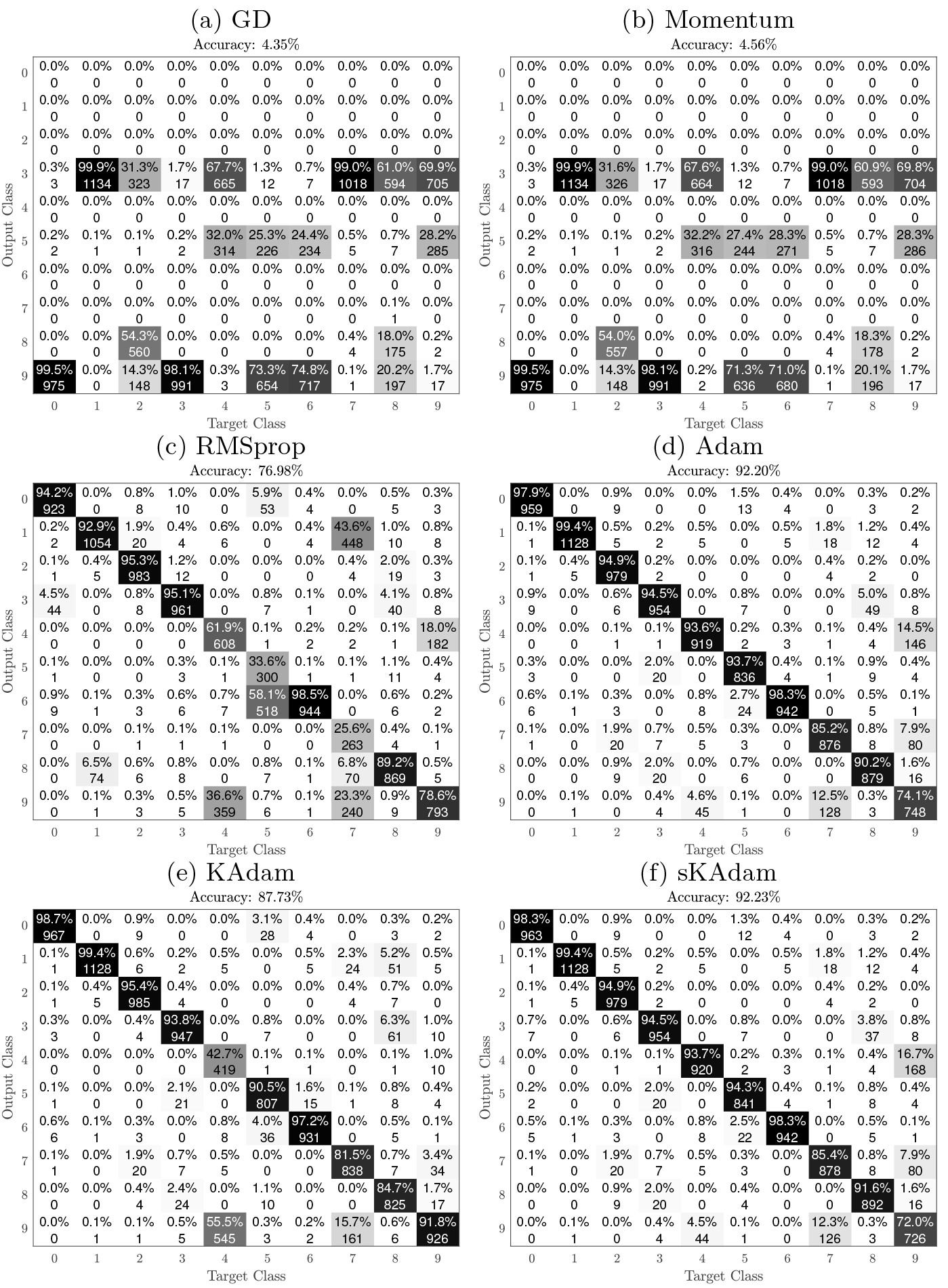
As it can be seen either in the comparisons and at the Table 1 of the experiment, the adaptive learning-rate methods as RMSProp, Adam, KAdam, and sKAdam present the best performance over the optimization. However, for the other methods, only the execution time is a remarkable feature in the comparison. Therefore in the following experiments, the gradient descent and momentum methods were removed from the comparison results.
In Fig. 5 it can be observed the confusion matrices from all the algorithms in the comparison. These matrices were calculated from the generalization performed with the trained neural networks in full-batch settings and using the test dataset, which contains 10,000 patterns.
Figure 5.
Confusion matrix for MNIST Generalization.
5.2Moon database classification experiment
In order to test the behavior of sKAdam with datasets that present a low noise factor, it was selected this experiment that deals with the classification problem of two interleaving half circles in two dimensions. The dataset contains 10,000 patterns, generated by a function22 from the scikit-learn python package [8].
The loss reduction comparison was run over 3,000 epochs and using a mini-batch size of 256. For the architecture of the neural networks, two layers were used with (10, 1) neurons, hyperbolic tangent and sigmoid as the activation functions respectively.
In Fig. 6, it can be seen again that using mini-batch settings sKAdam presents a smother behavior and is dampening the oscillations that KAdam presents during the training. Thus, sKAdam confirms again that as the authors state out when the exponential decay is used over the measurement noise factor the new method does not present the noisy behavior later in training.
Figure 6.
Moons optimization in mini-batch settings – comparison of the loss reduction over the trainings.
On the other hand, Fig. 7 shows that using full-batch settings there is not a remarkable difference in the performance from all the algorithms.
Figure 7.
Moons optimization in full-batch settings – comparison of the loss reduction over the trainings.
Nevertheless, in the summarize presented on Table 2 it is confirmed that KAdam and sKAdam present a considerable difference in the time taken to optimize even in full-batch settings due to the matrix inverse computed in KAdam vs the simpler calculation of the scalar multiplicative inverse that sKAdam performs. In Table 2, the columns min. loss present the minimum value for the loss function found for each algorithm, the columns min
Table 2
Moons – Comparisons table
| Mini-batch | Full-batch | |||||
|---|---|---|---|---|---|---|
| Min. loss | Min | Time (s) | Min. loss | Min | Time (s) | |
| RMSProp | 1.1538e-04 | 3.2804e-06 | 32.834 | 5.2815e-04 | 5.5869e-04 | 20.412 |
| Adam | 1.1193e-04 | 5.5350e-04 | 32.897 | 5.2196e-04 | 5.5350e-04 | 20.312 |
| KAdam | 1.1573e-04 | 2.8339e-06 | 64.636 | 5.1727e-04 | 5.4726e-04 | 20.551 |
| sKAdam | 1.0697e-04 | 2.8119e-06 | 38.546 | 5.1459e-04 | 5.3887e-04 | 19.192 |
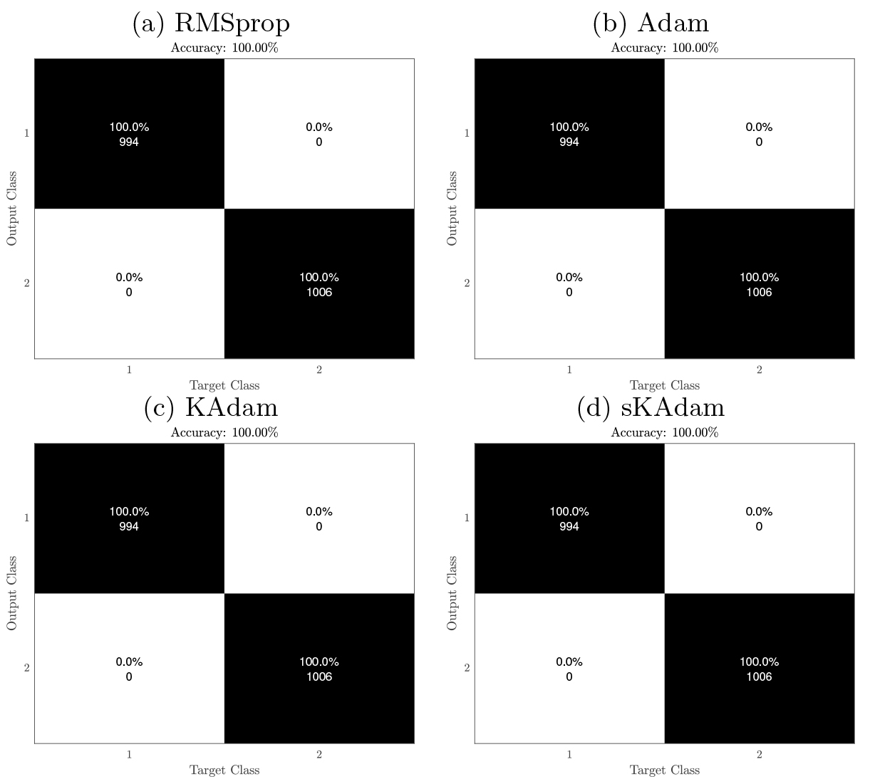
In Fig. 8 it can be observed the confusion matrices from all the algorithms in the comparison. These matrices were calculated from the generalization performed with the trained neural networks in full-batch settings and using the test dataset, which contains 2,000 patterns.
Figure 8.
Confusion matrix for Moon Generalization.
5.3Iris database classification experiment
One of the best-known dataset for pattern recognition. The problem (obtained from [4]) has four features (sepal length/width and petal length/width) to classify different iris plant species. In the classification, there are three different kinds of iris plants, but only one class is linearly separable from the others and also the latter are not linearly separable from each other. The dataset consists of 150 patterns (112 used for training) with 50 instances per class.
The loss reduction comparison was run over 1,000 epochs and using a mini-batch size of 32. For the architecture of the neural networks, two layers were used with (10, 3) neurons, hyperbolic tangent and sigmoid as the activation functions respectively.
As it can be observed in Fig. 9, this time in the mini-batch settings is where all the algorithms present close result in the loss function.
Figure 9.
Iris optimization in mini-batch settings – comparison of the loss reduction over the trainings.
On the other hand, Fig. 10 shows that in full-batch settings sKAdam presents a smoother behavior compared with RMSProp and KAdam. Moreover, it was able to make a significant change in the decent direction, thus, the algorithm presents a faster descent and a better accuracy in the loss reduction.
Figure 10.
Iris optimization in full-batch settings – comparison of the loss reduction over the trainings.
In Table 3, this time KAdam presents closer achievements in comparison with sKAdam. Nevertheless, in the mini-batch settings, the execution of KAdam takes nine times longer to finish the optimization due to the matrix inverse computed in KAdam vs the simpler calculation of the scalar multiplicative inverse that sKAdam performs. In Table 3, the columns min. loss present the minimum value for the loss function found for each algorithm, the columns min
Therefore, the execution time in KAdam increases as the the mini-batch size decrease. Thus, if its algorithm is used in a problem with a large numbers of patters and the optimization use mini-batch settings or online-settings, the problem of the execution time becomes serious.
Table 3
Iris classification – Comparisons table
| Mini-batch | Full-batch | |||||
|---|---|---|---|---|---|---|
| Min. loss | Min | Time (s) | Min. loss | Min | Time (s) | |
| RMSProp | 1.5366e-06 | 4.3371e-06 | 2.756 | 1.4322e-04 | 8.6790e-04 | 0.554 |
| Adam | 1.7771e-06 | 3.0501e-06 | 3.019 | 1.0876e-04 | 0.0011 | 0.927 |
| KAdam | 1.4457e-06 | 3.1983e-06 | 16.945 | 8.0615e-05 | 0.0011 | 2.897 |
| sKAdam | 1.0465e-06 | 2.7685e-06 | 4.894 | 8.2510e-05 | 9.0293e-04 | 0.737 |
Figure 11.
Confusion matrix for Iris Generalization.
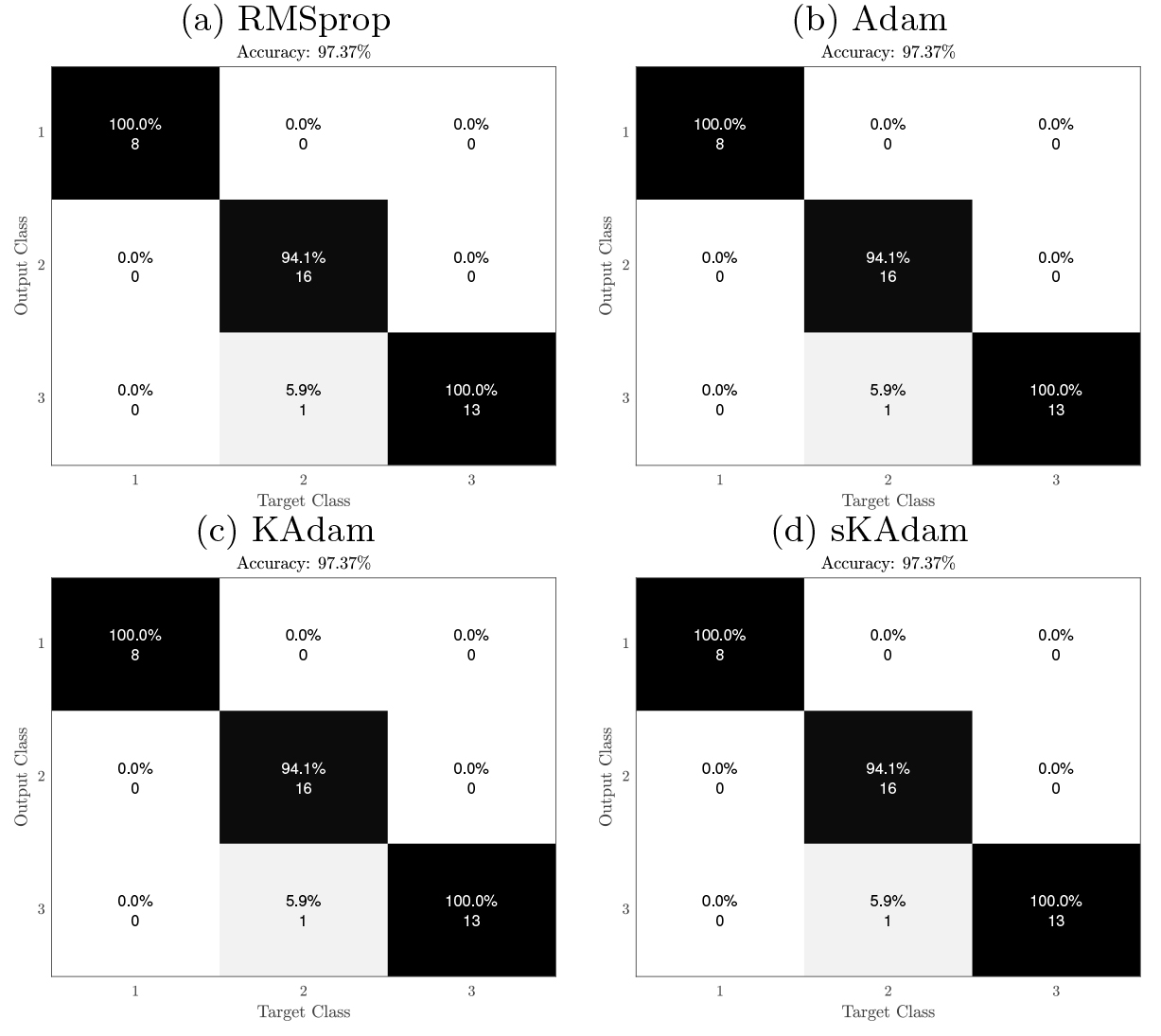
In Fig. 11 it can be observed the confusion matrices from all the algorithms in the comparison. These matrices were calculated from the generalization performed with the trained neural networks in full-batch settings and using the test dataset, which contains 38 patterns.
5.4Red wine quality regression/classification experiment
The regression/classification problem [3] for the quality of different wines. As an evaluation for the quality, there are 11 features related to physicochemical tests for each wine sample. The authors of the database shared two datasets related to the quality of different red and white wines. For this experiment, it was used the red wine dataset, which contains 1,599 samples (1,119 used for training).
The loss reduction comparison was run over 1,000 epochs and using a mini-batch size of 256. In the architectures of the neural networks, two layers were used with (20, 1) neurons, hyperbolic tangent and linear as the activation functions respectively. This experiment uses more hidden units with the objective of test the impact in the execution time.
Table 4
Red wine regression/classification – Comparisons table
| Mini-batch | Full-batch | |||||||
|---|---|---|---|---|---|---|---|---|
| Min. loss | Min | Time (s) | Min. loss | Min | Time (s) | |||
| RMSProp | 0.3924 | 0.1201 | 0.192 | 6.178 | 0.5000 | 18.6271 | 0.175 | 6.028 |
| Adam | 0.3762 | 0.1075 | 0.319 | 5.956 | 0.5630 | 19.0973 | 0.343 | 5.794 |
| KAdam | 0.3800 | 0.1031 | 0.323 | 241.950 | 0.5545 | 18.8704 | 0.141 | 55.067 |
| sKAdam | 0.3780 | 0.0162 | 0.356 | 7.615 | 0.4349 | 1.6257 | 0.359 | 7.150 |
Figure 12.
Red wine optimization in mini-batch settings – comparison of the loss reduction over the trainings.
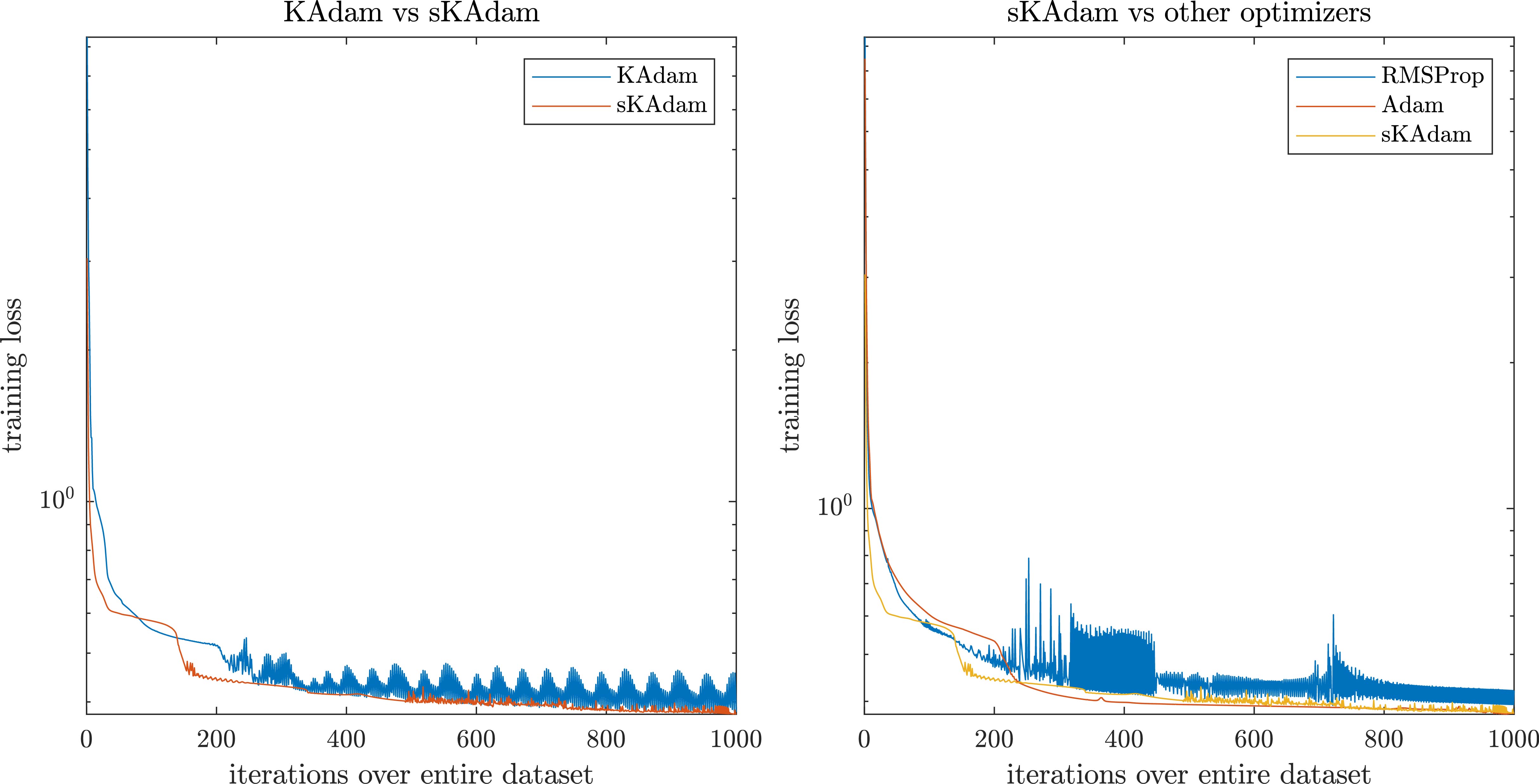
As Fig. 12 shows, in the mini-batch settings sKAdam presents a smoother and fastest descent compared with the other methods. Moreover, when all the algorithms present problems to reach low values over the loss function, our method was able to find a new and better solution even latter in training.
On the other hand, it can be seen in Fig. 13 that in full-batch settings sKAdam was close to the other methods, but near to the epoch 300 the algorithm find a new solution and it takes the advantage up to the end of the optimization.
Figure 13.
Red wine optimization in full-batch settings – comparison of the loss reduction over the trainings.
It can be seen in Table 4 that the architecture used in this experiment increase dramatically the execution time for the KAdam’s algorithm in both mini-batch and full-batch settings due to the matrix inverse computed in KAdam vs the simpler calculation of the scalar multiplicative inverse that sKAdam performs.
Furthermore, it can be observed that sKAdam does not present this problem and also handles to find new solutions over the loss function almost in the same execution time that the other optimizers.
In Table 4, the columns min. loss present the minimum value for the loss function found for each algorithm, the columns min
6.Conclusions
In this work, it was presented a new version of our state-of-the-art gradient-based optimizer. An extension of KAdam improved with the scalar Kalman filter and an exponential decay over the noise considered in the measurement process. This allows the algorithm to explore in a fraction of the optimization as well as keep following the original gradients later in training, aiming to find new and potentially better solutions.
As it has been shown with our new proposed method, it was overpassed the problem of the inverse matrix from the KAdam algorithm by using scalar operations with 1-D Kalman filters. This allows sKAdam to present a great performance in mini-batch and full-batch settings almost in the same execution time as well as present the fastest descent and reach lower values over the loss function. Furthermore, with the datasets of the experiments, it is confirmed that our proposal is well-suited for problems with large data-sets, noisy and/or sparse gradients, and non-stationary objectives.
For future work, the authors want to extend this work using the proposal in deep neural networks and with famous architectures like the ResNet.
Notes
2 https://scikit-learn.org/stable/modules/generated/sklearn.datasets.make_moons.html – using a noise factor of 0.05.
Acknowledgments
The authors thank the support of CONACYT Mexico, through Projects CB256769 and 443 CB258068 (“Project supported by Fondo Sectorial de Investigación para la Educación”) and PN-4107 (“Problemas Nacionales”).
References
[1] | J.C. Duchi, E. Hazan and Y. Singer, Adaptive subgradient methods for online learning and stochastic optimization, Journal of Machine Learning Research 12: ((2011) ), 2121–2159. |
[2] | J.D. Camacho, C. Villaseñor, A.Y. Alanis, C. Lopez-Franco and N. Arana-Daniel, Kadam: Using the kalman filter to improve adam algorithm, in: I. Nyström, Y. Hernández Heredia and V. Milián Nú nez, editors, Progress in Pattern Recognition, Image Analysis, Computer Vision, and Applications, Cham, Springer International Publishing, (2019) , pp. 429–438. |
[3] | P. Cortez, A. Cerdeira, F. Almeida, T. Matos and J. Reis, Modeling wine preferences by data mining from physicochemical properties, Decis Support Syst 47: (4) (Nov. (2009) ), 547–553. |
[4] | D. Dua and C. Graff, UCI machine learning repository, (2017) . |
[5] | R.E. Kalman, A new approach to linear filtering and prediction problems, Transactions of the ASME–Journal of Basic Engineering 82: (Series D) ((1960) ), 35–45. |
[6] | D.P. Kingma and J. Ba, Adam: A method for stochastic optimization, In 3rd International Conference on Learning Representations, ICLR 2015, San Diego, CA, USA, May 7–9, 2015, Conference Track Proceedings, (2015) . |
[7] | A. Neelakantan, L. Vilnis, Q.V. Le, I. Sutskever, L. Kaiser, K. Kurach and J. Martens, Adding gradient noise improves learning for very deep networks, CoRR, abs/1511.06807, (2015) . |
[8] | F. Pedregosa, G. Varoquaux, A. Gramfort, V. Michel, B. Thirion, O. Grisel, M. Blondel, P. Prettenhofer, R. Weiss, V. Dubourg, J. Vanderplas, A. Passos, D. Cournapeau, M. Brucher, M. Perrot and E. Duchesnay, Scikit-learn: Machine learning in Python, Journal of Machine Learning Research 12: ((2011) ), 2825–2830. |
[9] | N. Qian, On the momentum term in gradient descent learning algorithms, Neural Networks 12: (1) ((1999) ), 145–151. |
[10] | S. Ruder, An overview of gradient descent optimization algorithms, CoRR, abs/1609.04747, (2016) . |
[11] | T. Tieleman and G. Hinton, Lecture 6.5 – RMSProp, Technical report, COURSERA: Neural Networks for Machine Learning, (2012) . |
[12] | L. van der Maaten and G. Hinton, Visualizing data using t-sne, Journal of Machine Learning Research 9: ((2008) ), 2579–2605. |
[13] | M.D. Zeiler, ADADELTA: An adaptive learning rate method, CoRR abs/1212.5701 ((2012) ). |


