
Highly compressed image representation for classification and content retrieval
Abstract
In this paper, we propose a new method of representing images using highly compressed features for classification and image content retrieval – called PCA-ResFeats. They are obtained by fusing high- and low-level features from the outputs of ResNet-50 residual blocks and applying to them principal component analysis, which leads to a significant reduction in dimensionality. Further on, by applying a floating-point compression, we are able to reduce the memory required to store a single image by up to 1,200 times compared to jpg images and 220 times compared to features obtained by simple output fusion of ResNet-50. As a result, the representation of a single image from the dataset can be as low as 35 bytes on average. In comparison with the classification results on features from fusion of the last ResNet-50 residual block, we achieve a comparable accuracy (no worse than five percentage points), while preserving two orders of magnitude data compression. We also tested our method in the content-based image retrieval task, achieving better results than other known methods using sparse features. Moreover, our method enables the creation of concise summaries of image content, which can find numerous applications in databases.
1.Introduction
With virtually unlimited access to information, storing large amounts of data becomes increasingly problematic. For example, images from surveillance cameras must be overwritten due to a lack of adequate storage resources. Image datasets used in data science or video require terabytes of storage capacity to store on disks. However, such images often contain unnecessary, redundant information that can be removed to achieve significant compression while preserving the most essential information. In many classification tasks, storing the original image datasets on which classifiers are trained is unnecessary or these datasets can be offloaded to other cheaper but slower media [1]. Ultimately, the image representations given at the input are sufficient to receive the corresponding label at the output. Storing a less dimensional and compressed representation of the originals can help reduce the required storage volumes and allow a much larger number of examples to be stored, with no apparent impact on classification performance. As regards to sparse representation of images, not only the storage space is essential, but also the processing time. An example is content-based image retrieval (CBIR), which we also address in this paper. In this task, a common scenario is that a subset of the most similar representations is selected from many millions of images based on the highly compressed representations. Then, the whole process is repeated on the subset of less compact representations chosen in the previous iteration, allowing for more accurate matches and significantly reducing processing time. These two limitations, the huge storage usage of present-day datasets and the long processing time were the primary motivation for the works on the presented approach.
Such representations can be local sparse features that carry information in a very compact form, allowing inference about the image content. They can be used to search for common areas in different images, to determine camera positions, to combine photos into panoramas, or to perform 3D modeling. At the beginning of the 21st century, the most popular method for determining local features became the scale-invariant features transform (SIFT), proposed by David Lowe [2]. This work generated significant interest in sparse image descriptors and contributed to the development of many other methods. Currently, the field of image analysis is dominated by various types of neural networks [3, 4, 5, 6, 7, 8, 9, 10, 11, 12] and visual transformers [13]. We have demonstrated that the use of deep neural networks enables the construction local semantic descriptors which allow for more efficient image analysis and retrieval than known solutions.
In this paper, we propose a more compact and robust version of the ResFeats features proposed by Mahmood et al. [14, 15]. Our main contributions are as follows. First, we propose a set of dimensionality reduction methods for the original ResFeats, which count 3854 floating-point values each in their original form. In this context, we present and analyze (i) various combinations of features from output layers, (ii) principal component analysis (PCA) [16, 17], as well as (iii) feature sampling on combined high- and low-level ResNet-50 features. We also investigated (iv) the impact of a floating-point compression, called ZFP by its creators [18], on the proposed features. Second, we have extensively tested various setups in the classification tasks on six referential datasets and CBIR. The results show that the most promising is the combination of PCA with about 60 components and ZFP, which in some cases allows up to 220-fold reduction in memory consumption for the representation of features without significantly reducing or even increasing the accuracy of classification and CBIR results, as compared to other published methods.
2.Related works
The quest for the best-performing features has been the “Holy Grail” of the computer vision community for decades. We have experienced several breakthroughs in this field. After using different edge and corner detectors for a long period, the real breakthrough came in 2004 after D. Lowe published his seminal paper on the SIFT [2]. It gained many citations, as well as improvements and modifications, such as [19, 20], to name a few.
Exciting in the context of our work is the method by Ke and Sukthankar [19]. They proposed to employ PCA in the last step of the SIFT algorithm, that is, building a representation of key points based on patches. Thanks to this, the PCA-SIFT is constructed, which allowed not only for data reduction but – in many cases – also for increased classification accuracy.
The great success of SIFT spawned research in the field of sparse image descriptors and resulted in many improvements and similar methods. For example, we can mention here the speeded-up robust features method (SURF) [21], keypoint detector Features from Accelerated and Segments Test (FAST) [22], the Binary Robust Independent Elementary Feature detector (BRIEF) [23], as well as their follow-up oriented FAST and Rotated BRIEF (ORB) [24], then very efficient to compute densely DAISY [25, 26], or in the other group – the scale and affine invariant features by Mikolajczyk and Schmid [27], as well as histograms of oriented gradients (HOG) [28, 29], to name a few. However, in recent years, deep neural networks have shown their superiority also in the computation of local descriptors and sparse features for such tasks as image classification or content retrieval.
In the work of Mihai Dusmanu et al. [30], a D2-Net architecture is proposed that finds reliable keypoints under challenging imaging conditions. The approach presented there assigns a dual role to a single convolutional neural network (CNN): it is both a feature descriptor and a feature detector. The backbone of the D2-Net network is a pretrained on ImageNet VGG16 network. The proposed method achieves promising results both on the difficult Aachen Day-Night dataset with photos of objects taken during both day and night and on the InLoc benchmark dataset with photos of building interiors. In 2022, a paper was published [31] that corrected two shortcomings of D2-Net: low positioning accuracy of detected keypoints and emphasis only on the repeatability of detected keypoints, which could lead to mismatches in areas with the same texture. To increase the invariance and the correctness of local descriptor matches counted based on CNN, a paper by Liang et al. [32] proposed a Multi-Level Feature Aggregation (MLFA) module for efficient information transfer between levels. Each level extracts a feature vector, and the final descriptor concatenates them. In addition, to exploit the spatial structure within a local image fragment, the authors proposed a Spatial Context Pyramid (SCP) module to capture spatial information. The algorithm was implemented based on the Harmonic Densely Connected Network (HarDNet) framework [33]. The results obtained by the authors show that their method compares favorably with state-of-the-art (SOTA) methods. Nevertheless, these require significant computational resources and memory for data storage. There are also approaches to representing a point cloud using a single feature vector. In [34], using Self-Organizing Map (SOM), the proposed SO-Net network performs hierarchical feature extraction at individual points and processes them into a feature vector.
A method that proposed PCA to be applied directly to the last semantic layer of ResNet-50 is investigated in [35]. It shows good results in classification with spares data representation. However, the size of the features is still a few kilobytes per image. We will refer to this method in a further part of this paper.
A very influential is the work by Mahmood et al. [14]. For global feature extraction of images the features of the last residual layer called Res5c of ResNet-50 trained on the ImageNet are proposed. These
Features extracted from deeper layers perform better than those from shallower layers. However, their size is also significant due to the size of these output layers, but also because these need to be represented in the floating-point format that consumes at least 4 bytes per feature. In this paper we address this issue, proposing new ways for this size reduction even by two orders of magnitude with comparable or even better performance than the original ResFeats.
Based on superpixels and feature fusion, the solution proposed in [36] uses a codebook of size 2048 or 1024. On the other hand, Arco et al. proposed a sparse coding approach [37]. The images are first divided into tiles, and after applying PCA to these tiles, a dictionary is created. The original signals are then transformed into a linear combination of dictionary elements. The technique presented in [38], on the other hand, reduces CNN layers through an iterative process of removing neurons from the layer and tuning the network. The method presented in [39] is based on the use of wavelet packet transform (WPT)/Dual-Tree Complex Wavelet Transform (DT-CWT) to transform images from the spatial domain to the wavelet domain. The selected channels are stacked to form a tensor of the
In this paper a method is proposed for global image feature computations of extremely compact representation than in any of the aforementioned reference papers. On the other hand, despite such a high compression ratio, the most essential information is retained that allows for the classification and CBIR tasks with results that favorably compare to the other works.
3.Proposed method
Based on the assumption that deep features extracted from ResNet-50 contain redundant information, we propose the following method for obtaining highly compressed image representations. First, we combine high-level and low-level features extracted from ResNet-50 residual network blocks (see Fig. 1). Then, we apply dimensionality reduction techniques to these features. Finally, we also check the effect of lossy floating-point ZFP compression on the classification of these compact features. This allows us to store highly compressed datasets that still maintain information sufficient for high accuracy image classification or retrieval.
Figure 1.
A scheme of the ResNet-50 network architecture and subsequent ResFeats extraction layers. Adapted from [15].
![A scheme of the ResNet-50 network architecture and subsequent ResFeats extraction layers. Adapted from [15].](https://ip.ios.semcs.net:443/media/ica/2024/31-3/ica-31-3-ica230729/ica-31-ica230729-g001.jpg)
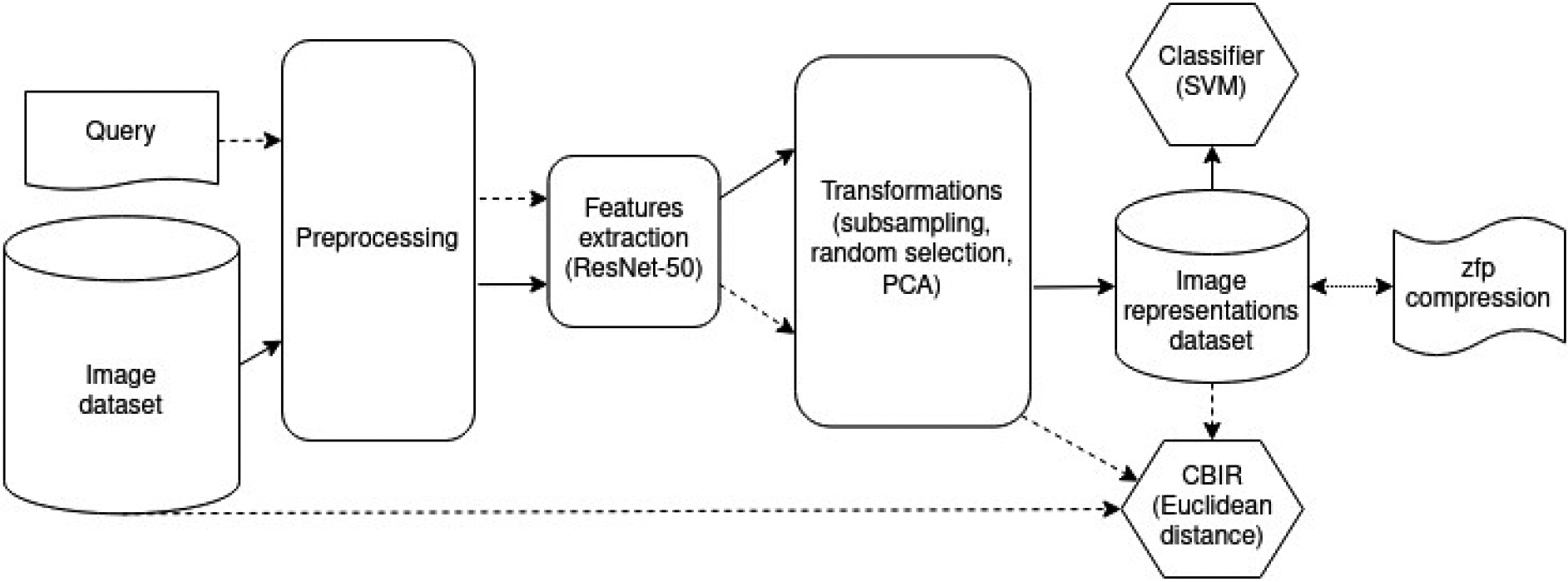
Figure 2.
A general picture of the proposed approach. The regular arrows indicate the data flow in the classification task, and the arrows with a dashed line show the data flow in the CBIR task. ZFP compression is performed on a dataset of image representations.
This work skillfully combines several concepts, approaches, techniques and components. Specifically, our main contributions are as follows.
• Investigations of various combinations of features from the (2), (3), and (4) layers of ResNet-50 and feature sampling;
• Application of PCA to various combinations of features from the (2), (3), and (4) layers of ResNet-50 that allows even two orders of magnitude size reduction – we call the new features PCA-ResFeats;
• Investigation of the floating-point compression methods to PCA-ResFeats for further required memory reduction and potential use for computing summaries of datasets. In this respect, we applied and verified (i) 32-bit to 16-bit conversion, as well as (ii) application of the ZFP method;
• Verification of PCA-ResFeats in the classification tasks of various datasets;
• Verification of PCA-ResFeats in the CBIR problem.
Figure 3.
A schematic of the ResNet-50 network architecture and various feature extraction layers used in this paper. (4a) is the ResNet-50 layer after the last average-pool block and before the fully connected one. ResFeats are composed of the (2)
![A schematic of the ResNet-50 network architecture and various feature extraction layers used in this paper. (4a) is the ResNet-50 layer after the last average-pool block and before the fully connected one. ResFeats are composed of the (2) + (3) + (4) layers, which come after the max-pool blocks. Adapted from [44].](https://ip.ios.semcs.net:443/media/ica/2024/31-3/ica-31-3-ica230729/ica-31-ica230729-g003.jpg)
A general picture of the proposed approach is shown in Fig. 2. The regular arrows indicate the data flow in the classification task, and the arrows with a dashed line show the data flow in the CBIR task. ZFP compression is performed on a dataset of image representations. The use of this compression will further reduce the necessary storage. Hence, a possible use-case scenario of our method is as follows: a database with a large number of images can be stored on a cheaper but slower medium (such as ’old’ tape technology, now reconsidered as a remedy for energy conservation [1]), while much smaller representations compressed by our method can be stored on faster media (such as SSD). Then various classification and/or data retrieval tasks, even not known at the time of PCA-ResFeat off-line computation, can be performed exclusively with the latter much more compact representation. In the next step, however, if one wishes to retrieve the original images, then these are available after an access to the former, slower database representation. All this at high speed and ensuring higher data protection during processing original data.
Another example of using our approach could be searching for particular video content based on a limited number of frames. Namely, instead of searching through the huge database with original videos (such as YouTube), we can just quickly search through the much smaller video representations in the form of our proposed PCA-ResFeats. Then, only the suitable videos in which a match was found can be retrieved from the original repository.
Since our starting setup is identical to the one from [15], we omit the exact description of the method of obtaining ResFeats features here. Nevertheless, the reader interested in the details of ResNet-50 can refer to publication [11], while the description of base ResFeats and the used SVM classifier is in [15, 17].
The following subsections describe the details of the aforementioned feature preprocessing methods.
3.132-bit to 16-bit floating-point conversion
The outputs of successive residual units of the residual neural network ResNet-50 pretreated on the ImageNet, used to extract ResFeats, are stored in the 32-bit floating-point (float32) representation [43]. Using data conversion from float32 to float16, should halve the memory size required to store image representations. However, this reduction may adversely affect the classification results. The experiments are designed to determine whether the increased efficiency due to this type of conversion comes at the cost of decreased accuracy during classification.
3.2Selection of a subset of ResFeats coordinates
Mahmood et al. in [15] proposed to concatenate the outputs of the second (2), third (3), and fourth (4) residual units of the ResNet-50 network after the max pooling operation, which have lengths 512, 1024 and 2048, respectively. For more information about ResFeats, our study compared classification results obtained with various variants of ResFeats. Namely, we investigated feature vectors formed by concatenating the outputs of third (3) and fourth (4), second (2) and fourth (4), as well as second (2) and third (3) of the residual block. The corresponding tensors with lengths of 3072, 2560, and 1536 respectively – carry more information than the outputs separately and may contain less noise than the original ResFeats. Using them would reduce the memory needed to store the image representations by about 14%, 29%, and 57%, respectively. Figure 3 shows the simplified ResNet-50 architecture and the extraction locations of ResFeats and their proposed modifications. In addition to the new features from the fusion layers of ResNet-50, the experimental results of selecting a subset of ResFeats vector coordinates by randomizing and sampling each
Table 1
Essential information about the datasets used in the experiments, such as the number of classes (classes), the number of samples given in thousands (samples [in K]), the size of the smallest class (min class size), the size of the images (image size), and the difficulty of the dataset (difficulty)
| Dataset | Classes | Samples [in K] | Min class size | Image size | Difficulty |
|---|---|---|---|---|---|
| MLC2008 | 9 | 43 | 471 | 312 | Complex |
| EuroSAT | 10 | 27 | 2000 | 64 | Medium |
| Caltech-101 | 101 | 9 | 31 | Varied | Medium |
| Caltech-256 | 256 | 30 | 80 | Varied | Complex |
| Oxford Flowers | 102 | 8 | 40 | Varied | Medium |
| Dog vs Cat | 2 | 25 | 12500 | Varied | Simple |
3.3PCA-ResFeats =
A well-known technique for data dimensionality reduction is the principal component analysis (PCA) [16, 17, 29]. Since applying this method to the SIFT [19] allowed to increase the efficiency, given the suspected correlation of the data in the tensors of ResFeats, our proposition is to employ PCA also in this case. The study aimed to find the number of components for which the classification results on most of the datasets proposed for the evaluation would decrease by about five percentage points relative to those obtained with the ResNet-50 output (4a).
3.4Floating-point compression of PCA-ResFeats
The necessity of feature representation in the floating-point (FP) format is a frequently overlooked property. This negatively influences the size of the output representation since the common FP representations occupy either 8 or 4 bytes. In effect, also the response time is negatively affected. Hence, to reduce the memory needed to store image representations, apart from the PCA, we also propose the use of the ZFP compression method, initially presented by Lindstrom et al. to computer graphics applications [45, 18, 46]. It is a lossy method for compressing tensors with FP values, where it is possible to set up the maximum acceptable error threshold for a single FP value in a tensor compared to its decompressed value. As shown, ZFP compression significantly reduces the memory required to store floating-point data. Our method proposes the use of ZFP for PCA-ResFeats. Analysis of the classification results on the representations after decompression compared to those obtained without compression will determine whether the losses resulting from its application have a significant impact. Another advantage of the ZFP method is its ability to recover a single value from the compressed representation, i.e. it is not necessary to decompress the entire representation.
4.Experiments
4.1Datasets
Six datasets were used to determine the quality of image classification methods. Four of them were used by the authors [14, 15]. These are: MLC2008, Caltech-101, Caltech-256, Oxford Flowers. We added the EuroSAT and Dog vs Cat datasets. These last two datasets were selected for further evaluation because they are from different domains and have different difficulty levels. Table 1 provides a summary of information about the datasets used in the experiments, such as the number of classes, the number of samples given in thousands, the size of the smallest class, the size of the images, and the difficulty of the dataset.
4.2Experimental settings
Some datasets proposed for evaluation are imbalanced, which negatively affects the classification. To perform the classification, we balanced these datasets as follows: we performed 10 draws
4.3Classification
Following the original work on ResFeats [14, 15], the same type of classifier, SVM, with a linear kernel and the accuracy metric were also used. During the initial research, dozens of experiments were performed with different SVM kernels: linear, radial (RBF), polynomial, and sigmoid. However, the results did not show that any kernels performed noticeably better. Therefore, in this work we only present results with a linear kernel.
4.4Results
In the following results, we refer to the ResFeats as features obtained after max-pooling and concatenating the outputs of any ResNet-50 residual units. In contrast, the basic ResFeats refer to concatenation of exactly (2)
4.4.1Various combinations of ResFeats
The results of different ResFeats combinations are compared in Table 2. The output of the ResNet-50 network (column 4a), often used for feature extraction, was compared with various variants (the numbers in the column name indicate the numbers of the residual units whose outputs were used for extraction). Basic ResFeats [15] is placed in the last column.
Table 2
Classification results for various ResFeats combinations on six datasets. (4a) denotes only the last layer of ResNet-50 after the average-pooling (i.e., “standard” ResNet-50 feature extraction); all others are combinations of (2), (3), and (4) layers after the max-pooling; the last combination 2_3_4 denotes the basic ResFeats, described in [15]
| Dataset | 4a | 2_3 | 2_4 | 3_4 | 2_3_4 |
|---|---|---|---|---|---|
| MLC2008 | 72.48 | 73.42 | 68.35 | 68.90 | 68.86 |
| EuroSAT | 95.12 | 95.59 | 93.35 | 93.53 | 93.70 |
| Caltech-101 | 90.10 | 84.14 | 90.32 | 90.23 | 90.58 |
| Caltech-256 | 83.72 | 72.92 | 83.97 | 84.05 | 84.04 |
| Oxford Flowers | 91.24 | 94.11 | 91.67 | 91.92 | 91.93 |
| Dog vs Cat | 98.99 | 97.25 | 98.89 | 98.89 | 98.90 |
The best results were obtained (for half of the datasets) for concatenated outputs of the second and third residual units. Subsequent layers of the residual units convey different information, so their combinations may provide better results, depending on the tested dataset. Results in Table 2 indicate that the first choice can be just the combination (2)
Several thousand experiments have shown that storing data in the float16 type, as compared to the float32, has a negligible effect on the classification results, so all subsequent experiments were conducted only with the former representation, simply due to a smaller size (compression of the representation by half).
4.4.2Selection of a subset of ResFeats coordinates and PCA
Since it was suspected that ResFeats convey redundant information, appropriate techniques to reduce their size were used. For ease of comparison, let
Figure 4.
A comparison of classification results on various datasets depending on the dimensionality reduction factor
Figure 5.
A comparison of classification results on datasets depending on the dimensionality reduction factor
For all datasets, the best results were obtained by using PCA. Increasing the dimensionality reduction causes a decrease in the classification results, while it happens the slowest with PCA. Reducing the feature vector by 60 times for almost all datasets (except for Caltech-256, where the result is slightly lower) does not cause a decrease in accuracy below the previously assumed five percentage points threshold. Moreover, for half of the datasets (the simpler ones), even after reducing the feature vector 100 times, the results remain similar to those obtained with the basic ResFeats. On the other hand, choosing a subset of the coordinates of the feature vector gives lower results, while it is usually better to randomize a subset of coordinates than to take every
Table 3
Classification results on the data obtained after decompression of ZFP compressed PCA-ResFeats with 60 components and the tolerance
|
|
| 0.01 | 0.05 | 0.1 | 0.5 | 1 | 5 | 10 | 50 | 100 |
|---|---|---|---|---|---|---|---|---|---|---|
| MLC2008 | 69.20 | 69.21 | 69.19 | 69.21 | 69.25 | 69.24 | 69.26 | 69.41 | 69.33 | 66.41 |
| EuroSAT | 93.00 | 93.00 | 93.00 | 92.99 | 92.98 | 93.00 | 93.02 | 93.08 | 92.98 | 91.54 |
| Caltech-101 | 86.62 | 86.62 | 86.62 | 86.63 | 86.65 | 86.63 | 86.57 | 86.50 | 85.19 | 81.59 |
| Caltech-256 | 76.90 | 76.90 | 76.91 | 76.90 | 76.90 | 76.89 | 76.84 | 76.78 | 75.10 | 70.75 |
| Oxford Flowers | 90.75 | 90.75 | 90.75 | 90.75 | 90.73 | 90.76 | 90.71 | 90.55 | 88.34 | 82.40 |
| Dog vs Cat | 99.13 | 99.13 | 99.13 | 99.13 | 99.13 | 99.12 | 99.13 | 99.13 | 99.10 | 98.88 |
Table 4
Compression ratios of ZFP PCA-ResFeats representations, depending on the tolerance
|
| 0.01 | 0.05 | 0.1 | 0.5 | 1 | 5 | 10 | 50 | 100 |
|---|---|---|---|---|---|---|---|---|---|
| MLC2008 | 2.20 | 2.55 | 2.78 | 3.75 | 4.25 | 5.79 | 7.08 | 12.82 | 20.95 |
| EuroSAT | 2.22 | 2.58 | 2.81 | 3.81 | 4.32 | 5.92 | 7.26 | 13.43 | 22.15 |
| Caltech-101 | 2.20 | 2.55 | 2.77 | 3.73 | 4.23 | 5.75 | 7.01 | 12.60 | 20.60 |
| Caltech-256 | 2.20 | 2.55 | 2.78 | 3.75 | 4.25 | 5.79 | 7.07 | 12.79 | 21.09 |
| Oxford Flowers | 2.21 | 2.56 | 2.78 | 3.76 | 4.26 | 5.81 | 7.11 | 12.92 | 21.32 |
| Dog vs Cat | 2.19 | 2.54 | 2.75 | 3.71 | 4.20 | 5.69 | 6.93 | 12.32 | 20.20 |
As in previous experiments on the MLC2008 and EuroSAT datasets, the PCA-ResFeats classification achieved the best results for combinations of outputs from the second (2) and third (3) residual units. Unfortunately, for the more difficult two Caltech datasets, significantly lower results were obtained. The results of the other feature combinations are close to each other. Reducing the feature vector by 60 times compared to the basic ResFeats, using PCA (to get 60 components that explain most of the variance), results in no more than the assumed five percentage point deterioration away from classification with the (4a) layer (i.e., ResNet-50 output before Fully Connected Layer) for all datasets, except for the most difficult Caltech-256, for which we got slightly worse results. This means that each image can be represented by 60 float16 values, occupying only 120 bytes. This also means 120 times reduction of storage size compared to the basic ResFeats stored as float32. For the simplest set of Dog vs Cat, even after reducing the feature vector 100 times, i.e., selecting only the 36 most important components (only 72 bytes per image), the classification results are still at the same value as for the base ResFeats (i.e., about 99%). Thus, depending on a dataset, it is necessary to experimentally choose the best performing number of PCA-ResFeats components.
4.4.3Influence of the ZFP compression
To make the storage and transfer of the PCA-ResFeats representation even more compact, we propose to use the ZFP compression method of its floating-point values [45]. Since this is a lossy compression technique, a comparison was made to see how the classification results are affected by the compression ratio, which is controlled by a tolerance parameter. Namely, a tolerance of
Figure 6.
Comparison of classification results (with standard deviation bars) before ZFP compression (values in parentheses) and after decompression of ZFP compressed data, with a tolerance
Figure 6 shows a comparison of classification results (including standard deviations) after decompression of ZFP compressed data with a tolerance
4.5PCA-ResFeats in CBIR problem
PCA-ResFeats can be effectively used not only directly in the classification task but also in the well-known CBIR problem [48, 49]. Experiments were performed on the most challenging Caltech-256 dataset in two versions: balanced minimal (with 80 random images in each class, analogous to the previous classification task) and imbalanced (original). The datasets from both versions were divided into a training set and a test set in a ratio of 6:4 in 10 splits. On the training dataset, the images were preprocessed and passed through a network to determine the float16 basic ResFeats (2)
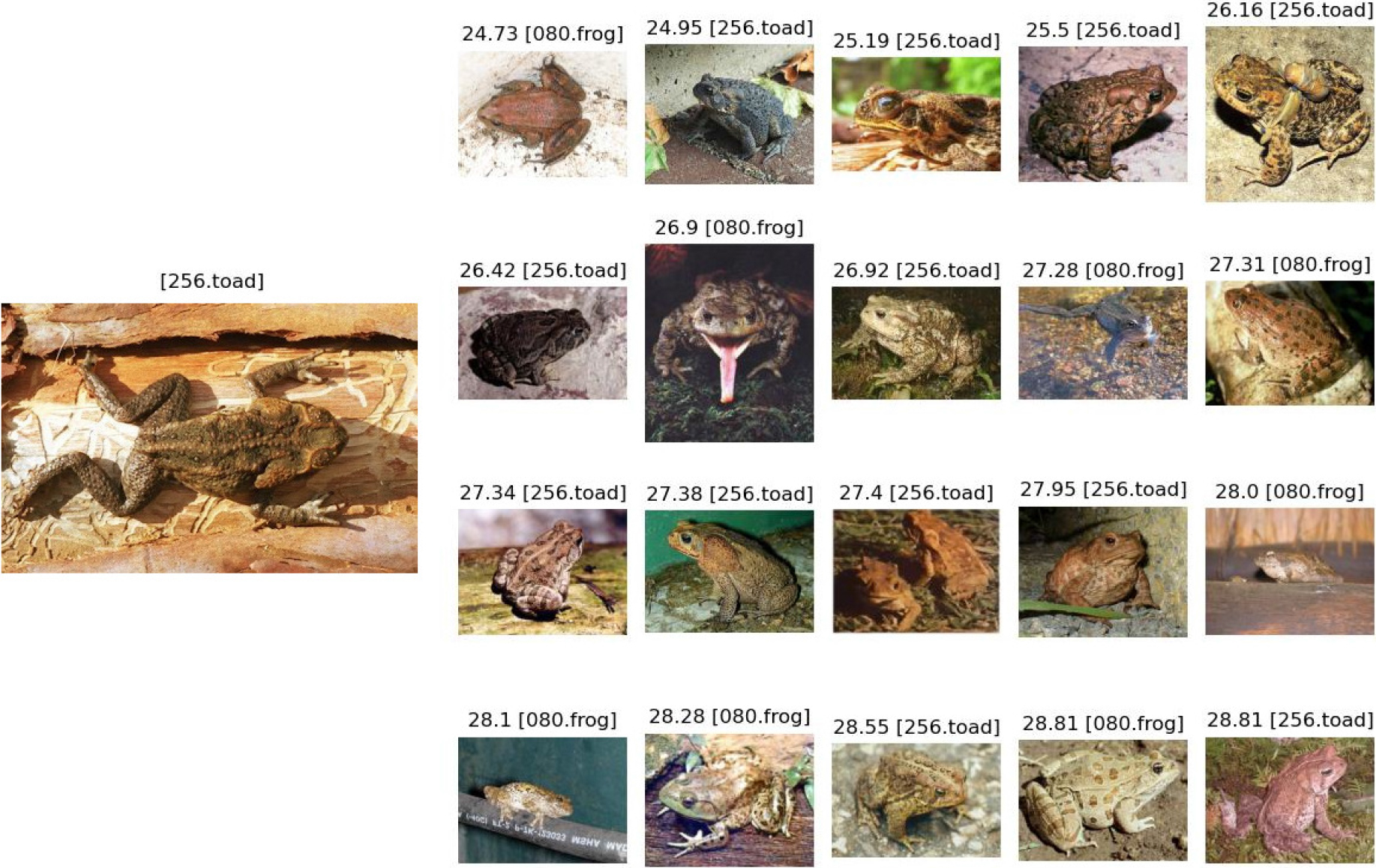
Figure 7.
On the left, the query image (256_0081.jpg) from the Caltech-256 toad class. On the right, the 20 images whose PCA-ResFeats were closest to the PCA-ResFeats obtained for the query. The distances and the classes of the examples are given above the images.
For evaluation, the metrics commonly used in the CBIR tasks were used: precision for
(1)
(2)
(3)
(4)
(5)
where
Table 5
MAP for the full and minimal version of Caltech-256, along with a comparison to SOTA method, for
| Caltech-256 | Full | Minimal | LB-CBIR [40] |
|---|---|---|---|
|
| 47.13% | 44.44% | |
|
| 51.77% | 44.44% | 32.12% |
| mAP | 46.73% | 43.02% |
Table 6
MAP results comparison on minimal Caltech-256 version
| Performance | PCAResFeats | BoW model [50] | Q-Way [51] | Dense SIFT [52] |
|---|---|---|---|---|
| MAP | 44.44%(43.02%) | 38.98% | 38.56% | 38.57% |
Figure 8.
MAP@k based on Eq. (3) (left) and based on Eq. (4) (right), as a function of requested first best responses

Figure 7 shows an example of a CBIR task. It presents the first 20 images with the smallest distance to the query image on the left. In this interesting case, just 60% of the responses indicate the correct class (i.e., “toad”), while the other returned images, not belonging to the valid class, are also “visually” similar and probably only an expert in the field can better distinguish between “toad” and “frog” classes.
The mAP (based on Eq. (5) for Caltech-256 reached 46.73% in the full version and 43.02% in the minimal (balanced) version. Figure 8 represents MAP@k from Eqs (3) and (4) respectively, as a function of the number
Table 6 compares the results of the proposed method based on PCA-ResFeats with other published methods used in the CBIR task for Caltech-256. The results clearly show that the proposed method performs about four percentage points better in the CBIR problem than other published methods, even choosing the least favorable way to compute MAP (43.02% vs. 38.98%). In addition, Caltech-256 contains very similar classes, such as “frog” and “toad”, as shown in Fig. 7.
5.Results and discussion
Based on the results, the proposed PCA-ResFeats with an experimentally determined length of 60 components are particularly interesting. Table 7 shows a cross-sectional summary of the averaged accuracy results obtained for the following classification variants:
• (4a) obtained from the output of the fourth residual unit ResNet-50, after average-pooling, of length 2048 and float16 type;
• (res) that are basic ResFeats of length 3584 and float16 type. The results from [15] for MLC2008, Caltech-101, Caltech-256, Oxford Flowers are 84.7%, 94.7%, 82.4%, 93.3% respectively;
• (2_3) obtained after concatenating the outputs of the second (2) and third (3) residual units after max-pooling, with a length of 1536 and float16 type;
• (4a_p60) obtained from the representation (4a) after PCA with 60 components, of length 60 and float16 type;
• (res_p60) that are PCA-ResFeats of length 60 and float16 type;
• (2_3_p60) obtained from the layers (2)
• (res_r60) obtained from the basic ResFeats, after drawing 60 features of float16 type;
• (res_s60) obtained from the layers (2)
Table 7
Comparison of classification results with variants of ResFeats on six datasets
| Dataset | Basic features | PCA-ResFeats | Sampled features | |||||
|---|---|---|---|---|---|---|---|---|
| Feature combination | 4a | res | 2_3 | 4a_p60 | res_p60 | 2_3_p60 | res_r60 | res_s60 |
| Feature vector length | 2048 | 3584 | 1536 | 60 | 60 | |||
| MLC2008 | 72.48 | 68.87 | 73.42 | 68.43 | 69.2 | 71.92 | 54.97 | 52.74 |
| EuroSAT | 95.13 | 93.70 | 95.59 | 92.58 | 93.00 | 94.35 | 81.75 | 83.22 |
| Caltech-101 | 90.10 | 90.58 | 84.14 | 87.17 | 86.62 | 75.38 | 57.92 | 55.95 |
| Caltech-256 | 83.72 | 84.03 | 72.92 | 78.25 | 76.90 | 59.95 | 47.79 | 46.27 |
| Oxford Flowers | 91.24 | 91.93 | 94.11 | 87.56 | 90.75 | 90.31 | 52.73 | 52.86 |
| Dog vs Cat | 98.99 | 98.90 | 97.25 | 99.09 | 99.13 | 97.61 | 95.63 | 95.67 |
Table 8
Comparison of our results with SOTA methods
| Dataset | S&FF [36] | ARC [38] | DTCWT | WPT | PCA-ResFeats |
|---|---|---|---|---|---|
| Caltech-101 | 74.50 | 83.20 | – | – | 87.17 |
| Caltech-256 | 43.33 | 77.50 | 72.24 | 71.02 | 78.25 |
Table 9
The storage (in MB) required to store images vs. PCA-ResFeats in different formats and representations; (ratio) denotes a ratio of memory used to store a dataset in zip format to the proposed ZFP format; (zfp_res_p60_acc) contains the accuracy obtained for the ZFP decompressed (res_p60) features
| Dataset | jpg | zip | res | res_p60 | zfp | ratio | zfp_res_p60_acc |
|---|---|---|---|---|---|---|---|
| MLC2008 | 65.835 | 66.005 | 24.321 | 0.407 | 0.115 | 574 | 69.41 |
| EuroSAT | 54.843 | 56.822 | 114.688 | 1.920 | 0.529 | 107 | 93.08 |
| Caltech-101 | 36.278 | 36.146 | 18.099 | 0.303 | 0.087 | 415 | 86.50 |
| Caltech-256 | 666.678 | 653.870 | 117.441 | 1.966 | 0.556 | 1176 | 76.78 |
| Oxford Flowers | 138.592 | 138.550 | 23.396 | 0.392 | 0.110 | 1260 | 90.55 |
| Dog vs Cat | 457.215 | 457.456 | 143.360 | 2.400 | 0.693 | 660 | 99.13 |
For half of the datasets, the best classification results were obtained for ResFeats extracted from the output of the second (2) and third (3) residual units. In addition, these features have the shortest length (compared to other combinations). However, the Caltech classification results are significantly worse than the other features. Therefore, in the case of these two complicated datasets, the best trade-off between accuracy and feature size is the output (4a) of ResNet-50 as the image representation since the classification results are closest to the best results.
Using PCA, dimensionality can be reduced by up to several orders of magnitude. Our research has shown that selecting only 60 principal components makes it possible to reduce memory by almost 60 times without classification accuracy drop by more than 5pp compared to the raw representation. The best results were obtained for PCA-ResFeats layers (2)
PCA-ResFeats can be further compressed using the ZFP method, in order to store their several times smaller representations. Table 9 shows how much disk space (in MB) is occupied by each training dataset (in which all classes have the same number of samples), in the following representations:
• (jpg) dataset in .jpg format;
• (zip) ZIP compressed (jpg) files;
• (res) data in the numpy (.npy) format, containing representations of images (basic ResFeats) in float16 type;
• (res_p60) proposed in this paper PCA-ResFeats, of length 60 and .npy format;
• (zfp) proposed in this paper PCA-ResFeats, in float32, then ZFP compressed with an
The column (ratio) shows the ratio between the storage used by the zipped dataset (zip) and used by the ZFP compressed PCA-ResFeats, with
By storing a dataset as ZFP compressed PCA-ResFeats with
The CBIR task completion time was also measured for the balanced Caltech-256. The results are as follows: it lasted 2593.44 seconds to perform CBIR on features extracted from the second, third, and fourth layers of ResNet-50 with a length of 3584. It lasted 49.14 seconds to perform the same experiment with additional PCA calculation and computation of PCA-Resfeats with a size of 60 from the basic features. It lasted just 45.55 seconds to perform the CBIR task on the cached PCA-Resfeats (without determining them). This means a more than 60-fold reduction in computation time and shows the advantage of using our proposed features for this task. A possible additional cost would be to refer to the database containing the original to return a user-interpretable image. However, it is more affordable than calculations performed on more extended features.
All experiments, but the CBIR, were repeated 100 times (10 random splits of datasets in each of the 10 drawn datasets) for each combination of the method and its parameters and six data sets. This gives the total number of more than 222,000 experiments. These have shown that our proposed PCA-ResFeats performs well in image classification sets while achieving a high compression ratio for the representation of these datasets.
The method also has potential practical applications. A huge image database can be stored hierarchically on a large storage device, disk, or tape (which is increasingly becoming a storage [1]). It is combined with a high-speed layer containing access to equivalent image representations (PCA-ResFeats). The experiments have shown that in such a case, it is worthwhile to perform CBIR on small but informative representations and then perform another search limited only to the images obtained in the previous step. Such a process can be repeated iteratively for representations compressed to varying degrees. With successive iterations, the number of examples returned can also be reduced, further optimizing the process. Using our approach can significantly speed up the entire process.
5.1Data and code availability
All accuracy values, averaged results with standard deviations, ZFP compression reports and also other CBIR images are available here: https://aghedupl-my.sharepoint.com/:f:/g/personal/slazewsk_agh_edu_pl/EpE8LQmXBIpDpVU44eYjuMYBMBCdbs3gO0EtEz9LIfo02w?e=TaumAv. We also provide a repository with code: https://github.com/Stanislaw-Lazewski/PCA-ResFeats.
The experiments were conducted on a server with an AMD Ryzen Threadripper 3990X 64-Core Processor. The code was written in Python using the Pytorch library.
6.Conclusions and future work
In this paper, we propose methods to improve the efficiency of image analysis using features derived from the ResNet-50 convolutional neural network – PCA-ResFeats. This is a significant extension and improvement of the results obtained by the method of Mahmood et al. [15]. Computation of PCA-ResFeats consists of several steps. First, ResFeats – feature vectors consisting of no more than 3584 floating-point values – are extracted as a concatenation of outputs (after max-pooling) of residual units of ResNet-50, pretrained on ImageNet. However, we also tested different combinations of the output layers, showing their usefulness. Then, thanks to PCA, we reduce the size of the feature vector to 60 floating-point values. Research has shown that they can be stored in the float16 format without losing information. The proposed technique gives classification accuracy not worse than 5pp when compared with much larger basic ResFeats on the benchmark datasets MLC2008, EuroSAT, Caltech-101, Caltech-256, Oxford Flowers or Dog vs Cat. At the same time, they achieve significant storage reduction.
The second contribution proposed in this paper is the further compression of PCA-ResFeats with the ZFP method. An additional 3.5 compression ratio and up to about 220-fold memory reduction can be achieved compared to storing basic ResFeats.
Our approach has also been tested in the CBIR task. For example, for the difficult dataset Caltech-256 using the proposed PCA-ResFeats with 60 components, results outperforming other published methods were obtained, and this is the third contribution of this paper. In conclusion, compared to other studies, the developed method of representing images with semantic local descriptors PCA-ResFeats, combined with the ZFP compression, achieved SOTA. It can also be successfully used to prepare summaries of datasets.
In the future, we will explore the use of other network architectures, such as densely connected convolutional networks (DenseNet) [53] or MobileNet [54, 55], as well as network ensembles [56], to extract raw features and see if they contain redundant information with little impact on classification. We will also test the application of our approach to medical data [57, 58, 59, 60]. We plan to generalize our approach to 3D representations of medical images [61], such as whole scan imaging (WSI) in histopathology. In this case, our approach can be very effective due to the enormous size of the WSI data. We will also compare the results of PCA-ResFeats extracted from the network pre-trained on ImageNet with those extracted from the network after fine-tuning the domain dataset. In this case, our method can be used in many other fields that use compact image representation, e.g. construction, various production lines, transport, autonomous vehicles, etc. [62, 63, 64, 65, 66]. The next subject of study will be a fusion of the features obtained from different neural networks. Another direction for future research may be the issue of image preprocessing. Perhaps the approach presented in [67] would enable the application of our method to thermal images. We can also explore the modern image binarization [68].
Acknowledgments
This work has been supported by the AGH University of Krakow under subvention funds no. 16.16.230.434.
References
[1] | Velvet Wu. Tape Storage Might Be Computing’s Climate Savior; (2023) . Online; accessed 15-October-2023. https://spectrum.ieee.org/tape-storage-sustainable-option. |
[2] | Lowe DG. Distinctive image features from scale-invariant keypoints. International Journal of Computer Vision. (2004) ; 60: (2): 91–110. |
[3] | Hung SL, Adeli H. A parallel genetic/neural network learning algorithm for MIMD shared memory machines. IEEE Transactions on Neural Networks. (1994) ; 5: (6): 900–909. |
[4] | Hung SL, Adeli H. Object-oriented backpropagation and its application to structural design. Neurocomputing. (1994) ; 6: (1): 45–55. |
[5] | Adeli H, Hung SL. Machine learning: neural networks, genetic algorithms, and fuzzy systems. John Wiley & Sons, Inc.; (1994) . |
[6] | Li H, Wang G, Lu J, Kiritsis D. Cognitive twin construction for system of systems operation based on semantic integration and high-level architecture. Integrated Computer-Aided Engineering. (2022) ; 29: (3): 277–295. |
[7] | Wu H, He F, Duan Y, Yan X. Perceptual metric-guided human image generation. Integrated Computer-Aided Engineering. (2022) ; 29: (2): 141–151. |
[8] | Hua Y, Shu X, Wang Z, Zhang L. Uncertainty-guided voxel-level supervised contrastive learning for semi-supervised medical image segmentation. International Journal of Neural Systems. (2022) ; 32: (04): 2250016. |
[9] | Wang K, Wang Y, Zhan B, Yang Y, Zu C, Wu X, et al. An efficient semi-supervised framework with multi-task and curriculum learning for medical image segmentation. International Journal of Neural Systems. (2022) ; 32: (09): 2250043. |
[10] | Alam KMR, Siddique N, Adeli H. A dynamic ensemble learning algorithm for neural networks. Neural Computing and Applications. (2020) ; 32: : 8675–8690. |
[11] | He K, Zhang X, Ren S, Sun J. Deep Residual Learning for Image Recognition. In: 2016 IEEE Conference on Computer Vision and Pattern Recognition (CVPR). (2016) . pp. 770–778. |
[12] | Ga̧sienica-Józkowy J, Knapik M, Cyganek B. An ensemble deep learning method with optimized weights for drone-based water rescue and surveillance. Integrated Computer-Aided Engineering. (2021) 01; 1–15. |
[13] | De Nardin A, Mishra P, Foresti GL, Piciarelli C. Masked transformer for image anomaly localization. International Journal of Neural Systems. (2022) ; 32: (07): 2250030. |
[14] | Mahmood A, Bennamoun M, An S, Sohel F. Resfeats: Residual network based features for image classification. In: 2017 IEEE International Conference on Image Processing (ICIP). IEEE; (2017) . pp. 1597–1601. |
[15] | Mahmood A, Bennamoun M, An S, Sohel F, Boussaid F. ResFeats: Residual network based features for underwater image classification. Image and Vision Computing. (2020) ; 93: : 103811. |
[16] | Jolliffe IT, Cadima J. Principal component analysis: A review and recent developments. Philos Trans A Math Phys Eng Sci. (2016) Apr; 374: (2065): 1–16. |
[17] | Cyganek B. Object detection and recognition in digital images: theory and practice. John Wiley & Sons; (2013) . |
[18] | Lindstrom P. Fixed-rate compressed floating-point arrays. IEEE Transactions on Visualization and Computer Graphics. (2014) ; 20: (12): 2674–2683. |
[19] | Ke Y, Sukthankar R. PCA-SIFT: A more distinctive representation for local image descriptors. In: Proceedings of the 2004 IEEE Computer Society Conference on Computer Vision and Pattern Recognition, 2004. CVPR 2004. vol. 2. IEEE; (2004) . pp. II–II. |
[20] | Arandjelović R, Zisserman A. Three things everyone should know to improve object retrieval. In: 2012 IEEE Conference on Computer Vision and Pattern Recognition. IEEE; (2012) . pp. 2911–2918. |
[21] | Bay H, Tuytelaars T, Van Gool L. SURF: Speeded Up Robust Features. In: Leonardis A, Bischof H, Pinz A, editors. Computer Vision – ECCV 2006. Berlin, Heidelberg: Springer Berlin Heidelberg; (2006) . pp. 404–417. |
[22] | Rosten E, Drummond T. Machine learning for high-speed corner detection. In: European Conference on Computer Vision. Springer; (2006) . pp. 430–443. |
[23] | Calonder M, Lepetit V, Strecha C, Fua P. Brief: Binary robust independent elementary features. In: European Conference on Computer Vision. Springer; (2010) . pp. 778–792. |
[24] | Rublee E, Rabaud V, Konolige K, Bradski G. ORB: An efficient alternative to SIFT or SURF. In: 2011 International Conference on Computer Vision. Ieee; (2011) . pp. 2564–2571. |
[25] | Tola E, Lepetit V, Fua P. DAISY: An efficient dense descriptor applied to wide-baseline stereo. IEEE Transactions on Pattern Analysis and Machine Intelligence. (2010) ; 32: (5): 815–830. |
[26] | Knapik M, Cyganek B. Comparison of Sparse Image Descriptors for Eyes Detection in Thermal Images. In: Proceedings of the 14th International Joint Conference on Computer Vision, Imaging and Computer Graphics Theory and Applications – Volume 5: VISAPP, INSTICC. SciTePress; (2019) . pp. 638–644. |
[27] | Mikolajczyk K, Schmid C. Scale & affine invariant interest point detectors. International Journal of Computer Vision. (2004) Oct; 60: (1): 63–86. Available from: doi: 10.1023/B:VISI.0000027790.02288.f2. |
[28] | Dalal N, Triggs B. Histograms of oriented gradients for human detection. In: 2005 IEEE Computer Society Conference on Computer Vision and Pattern Recognition (CVPR’05). vol. 1; (2005) . pp. 886–893. |
[29] | Bukała A, Koziarski M, Cyganek B, Koş ON, Kara A. The impact of distortions on the image recognition with histograms of oriented gradients. In: Image Processing and Communications: Techniques, Algorithms and Applications 11. Springer; (2020) . pp. 166–178. |
[30] | Dusmanu M, Rocco I, Pajdla T, Pollefeys M, Sivic J, Torii A, et al. D2-net: A trainable cnn for joint detection and description of local features. arXiv preprint arXiv:190503561. (2019) . |
[31] | Yang N, Han Y, Fang J, Zhong W, Xu A. UP-Net: Unique keyPoint description and detection net. Machine Vision and Applications. (2022) ; 33: (1): 1–13. |
[32] | Liang P, Ji H, Cheng E, Chai Y, Wang L, Ling H. Learning local descriptors with multi-level feature aggregation and spatial context pyramid. Neurocomputing. (2021) ; 461: : 99–108. |
[33] | Chao P, Kao CY, Ruan YS, Huang CH, Lin YL. HarDNet: A low memory traffic network. In: Proceedings of the IEEE/CVF International Conference on Computer Vision. (2019) . pp. 3552–3561. |
[34] | Li J, Chen BM, Lee GH. So-net: Self-organizing network for point cloud analysis. In: Proceedings of the IEEE Conference on Computer Vision and Pattern Recognition. (2018) . pp. 9397–9406. |
[35] | Koul A, Ganju S, Kasam M. Practical Deep Learning for Cloud, Mobile, and Edge: Real-World AI & Computer-Vision Projects Using Python, Keras & TensorFlow. O’Reilly Media; (2019) . |
[36] | Yang F, Ma Z, Xie M. Image classification with superpixels and feature fusion method. Journal of Electronic Science and Technology. (2021) ; 19: (1): 100096. |
[37] | Arco JE, Ortiz A, Ramírez J, Zhang YD, Górriz JM. Tiled sparse coding in eigenspaces for image classification. International Journal of Neural Systems. (2022) ; 32: (03): 2250007. |
[38] | Shah MA, Raj B. Deriving compact feature representations via annealed contraction. In: ICASSP 2020–2020 IEEE International Conference on Acoustics, Speech and Signal Processing (ICASSP). IEEE; (2020) . pp. 2068–2072. |
[39] | Wang L, Sun Y. Image classification using convolutional neural network with wavelet domain inputs. IET Image Processing. (2022) ; 16: (8): 2037–2048. |
[40] | Taheri F, Rahbar K, Salimi P. Effective features in content-based image retrieval from a combination of low-level features and deep Boltzmann machine. Multimedia Tools and Applications. (2022) ; 1–24. |
[41] | Fenton K, Bishop V, Simske S. Enhanced computer vision using automated optimized neural network image pre-processing. Archiving Conference. (2022) 06; 19: : 30–34. |
[42] | Grabek J, Cyganek B. An impact of tensor-based data compression methods on deep neural network accuracy. vol. 26; (2021) ; 3–11. |
[43] | Kukreja N. Python wrapper over the zfp compression library; (2019) . Available at https://pypi.org/project/pyzfp. |
[44] | Rastogi A. ResNet-50 Architecture; (2022) . Available at https://blog.devgenius.io/resnet50-6b42934db431. |
[45] | Lindstrom P. zfp: Compressed Floating-Point and Integer Arrays; (2019) . Available at https://computing.llnl.gov/projects/zfp. |
[46] | Diffenderfer J, Fox AL, Hittinger JA, Sanders G, Lindstrom PG. Error analysis of zfp compression for floating-point data. SIAM Journal on Scientific Computing. (2019) ; 41: (3): A1867–A1898. |
[47] | Pytorch Documentation TC. torchvision.models; (2017) . Online; accessed 15-October-2023. https://pytorch.org/vision/0.8/models.html. |
[48] | Gudivada VN, Raghavan VV. Content based image retrieval systems. Computer. (1995) ; 28: (9): 18–22. |
[49] | Vishraj R, Gupta S, Singh S. A comprehensive review of content-based image retrieval systems using deep learning and hand-crafted features in medical imaging: Research challenges and future directions. Computers and Electrical Engineering. (2022) ; 104: : 108450. |
[50] | Jabeen S, Mehmood Z, Mahmood T, Saba T, Rehman A, Mahmood MT. An effective content-based image retrieval technique for image visuals representation based on the bag-of-visual-words model. PloS one. (2018) ; 13: (4): e0194526. |
[51] | Mai TD, Ngo TD, Le DD, Duong DA, Hoang K, Satoh S. Efficient large-scale multi-class image classification by learning balanced trees. Computer Vision and Image Understanding. (2017) ; 156: : 151–161. |
[52] | Mai TD, Ngo TD, Le DD, Duong DA, Hoang K, Satoh S. Learning Balanced Trees for Large Scale Image Classification. In: Image Analysis and Processing – ICIAP 2015: 18th International Conference, Genoa, Italy, September 7–11, 2015, Proceedings, Part II 18. Springer; (2015) . pp. 3–13. |
[53] | Huang G, Liu Z, Van Der Maaten L, Weinberger KQ. Densely connected convolutional networks. In: Proceedings of the IEEE Conference on Computer Vision and Pattern Recognition. (2017) . pp. 4700–4708. |
[54] | Howard AG, Zhu M, Chen B, Kalenichenko D, Wang W, Weyand T, et al. Mobilenets: Efficient convolutional neural networks for mobile vision applications. arXiv preprint arXiv: 170404861. (2017) . |
[55] | Jodas DS, Yojo T, Brazolin S, Velasco GDN, Papa JP. Detection of trees on street-view images using a convolutional neural network. International Journal of Neural Systems. (2022) ; 32: (01): 2150042. |
[56] | Rafiei MH, Adeli H. A new neural dynamic classification algorithm. IEEE Transactions on Neural Networks and Learning Systems. (2017) ; 28: (12): 3074–3083. |
[57] | Nogay HS, Adeli H. Machine learning (ML) for the diagnosis of autism spectrum disorder (ASD) using brain imaging. Reviews in the Neurosciences. (2020) ; 31: (8): 825–841. |
[58] | Nogay HS, Adeli H. Detection of epileptic seizure using pretrained deep convolutional neural network and transfer learning. European Neurology. (2021) ; 83: (6): 602–614. |
[59] | Nogay HS, Adeli H. Diagnostic of autism spectrum disorder based on structural brain MRI images using, grid search optimization, and convolutional neural networks. Biomedical Signal Processing and Control. (2023) ; 79: : 104234. |
[60] | Rafiei MH, Gauthier LV, Adeli H, Takabi D. Self-supervised learning for electroencephalography. IEEE Transactions on Neural Networks and Learning Systems. (2022) . |
[61] | Li L, He F, Fan R, Fan B, Yan X. 3D reconstruction based on hierarchical reinforcement learning with transferability. Integrated Computer-Aided Engineering. (2023) ; (Preprint): 1–13. |
[62] | Xu Z, Zhang F, Wu Y, Yang Y, Wu Y. Building height calculation for an urban area based on street view images and deep learning. Computer-Aided Civil and Infrastructure Engineering. (2023) ; 38: (7): 892–906. |
[63] | Li D, Wu J, Zhu F, Chen T, Wong YD. Modeling adaptive platoon and reservation-based intersection control for connected and autonomous vehicles employing deep reinforcement learning. Computer-Aided Civil and Infrastructure Engineering. (2023) ; 38: (10): 1346–1364. |
[64] | Liu C, Xu N, Weng Z, Li Y, Du Y, Cao J. Effective pavement skid resistance measurement using multi-scale textures and deep fusion network. Computer-Aided Civil and Infrastructure Engineering. (2023) ; 38: (8): 1041–1058. |
[65] | Hassanpour A, Moradikia M, Adeli H, Khayami SR, Shamsinejadbabaki P. A novel end-to-end deep learning scheme for classifying multi-class motor imagery electroencephalography signals. Expert Systems. (2019) ; 36: (6): e12494. |
[66] | Martins GB, Papa JP, Adeli H. Deep learning techniques for recommender systems based on collaborative filtering. Expert Systems. (2020) ; 37: (6): e12647. |
[67] | Chaverot M, Carré M, Jourlin M, Bensrhair A, Grisel R. Improvement of small objects detection in thermal images. Integrated Computer-Aided Engineering. (2023) ; (Preprint): 1–15. |
[68] | Ćurković M, Ćurković A, Vučina D. Image binarization method for markers tracking in extreme light conditions. Integrated Computer-Aided Engineering. (2022) ; 29: (2): 175–188. |


