
Enhancing smart home appliance recognition with wavelet and scalogram analysis using data augmentation
Abstract
The development of smart homes, equipped with devices connected to the Internet of Things (IoT), has opened up new possibilities to monitor and control energy consumption. In this context, non-intrusive load monitoring (NILM) techniques have emerged as a promising solution for the disaggregation of total energy consumption into the consumption of individual appliances. The classification of electrical appliances in a smart home remains a challenging task for machine learning algorithms. In the present study, we propose comparing and evaluating the performance of two different algorithms, namely Multi-Label K-Nearest Neighbors (MLkNN) and Convolutional Neural Networks (CNN), for NILM in two different scenarios: without and with data augmentation (DAUG). Our results show how the classification results can be better interpreted by generating a scalogram image from the power consumption signal data and processing it with CNNs. The results indicate that the CNN model with the proposed data augmentation performed significantly higher, obtaining a mean F1-score of 0.484 (an improvement of
1.Introduction
In recent years, the increasing availability of smart homes has led to an explosion of data related to the use of household appliances. These data provide valuable information for many applications, such as predicting energy consumption, device fault detection, and user behavior analysis. Furthermore, with rising energy costs and growing concerns about climate change, there is a growing need for innovative solutions to help reduce energy waste and promote more sustainable energy use.
Accurate appliance recognition plays a crucial role in the realm of energy conservation [1]. Gaining a comprehensive understanding of the energy consumption patterns exhibited by individual appliances enables building managers and consumers to identify energy-saving opportunities and make informed decisions about their energy use. An in-depth study of appliance consumption patterns holds particular significance in this context. By disaggregating the power consumption data for each appliance, it becomes possible to identify the energy usage patterns of individual appliances, as well as the overall energy consumption of the household. This information can be used to develop more sophisticated energy management systems and provide personalized feedback to consumers, empowering them to make well-informed choices about their energy use and actively reduce their consumption. Emphasizing the importance of accurate appliance recognition as an integral part of energy conservation reinforces the importance of understanding and controlling energy consumption in the home.
The development of smart homes, equipped with devices connected to the Internet of Things (IoT) [2, 3], has opened up new possibilities for monitoring and controlling energy use. In this context, non-intrusive load monitoring (NILM) techniques have emerged as a promising solution for the disaggregation of total energy consumption into the consumption of individual appliances. Some studies indicate that it can help households save electricity [4, 5, 6, 7, 8]. For this reason, the analysis of the consumption of electrical energy by households has gradually become a research field that is attracting attention.
One of the most challenging tasks in NILM is to accurately identify the operation of each appliance. This problem has traditionally been tackled with supervised learning algorithms, such as k-Nearest Neighbors (kNN) and Support Vector Machines (SVM), among others [9, 10, 11, 12]. More recently, deep learning techniques [13, 14], such as Convolutional Neural Networks (CNNs) [15], or Long Short-Term Memory (LSTM), have shown promising results in NILM applications [16, 17, 18].
On the other hand, in the case of household appliances, a refrigerator that works 24 hours a day does not have the same use as a washing machine that is used more occasionally, resulting in a lack of sufficient labels for some appliances. When using classification algorithms, it is essential that the models know the behavior of all appliances. For this, sufficient samples are needed to represent the variability of the data in different situations.
Therefore, a data augmentation algorithm is recommendable, and, in our case, we compare the results with and without data augmentation. This data augmentation is based on generating new data by adding the consumption of appliances with other disaggregated energy consumption of household appliances in another time window. In this way, the model is trained to identify the appliance in other situations that would make it challenging to identify and allows one to obtain a model with better generalization.
In this work, we propose comparing and evaluating the performance of two different multiclass classification algorithms, namely Multi-Label K-Nearest Neighbors (MLkNN) and Convolutional Neural Networks (CNN), for NILM. This comparison will be carried out on two datasets: one original from the REDD dataset [19], and an augmented version of the same dataset. The augmented dataset aims to increase the variability of the original data and improve the generalizability of the algorithms. In addition, we will use the data in two different ways: on the one hand we will use the CWT which is a mathematical technique used to analyze signals or data in both the time and frequency domains, and provides a way to examine the time-varying frequency content of a signal at different scales. And on the other hand, we use scalograms which are a visual representation used in signal processing and time-frequency analysis. It is derived from the CWT and provides a way to analyze the frequency content of a signal over time. The scalogram is typically presented as a two-dimensional plot, where the vertical axis represents frequency and the horizontal axis represents time. It helps in identifying the presence of specific frequencies or patterns in a time-varying signal. Therefore, on one side we will use CWTs for MLkNN, and on the other side, scalograms to work with CNNs.
In summary, this paper presents three major contributions to the classification of disaggregated power consumption by appliance.
1. An innovative method for enhancing the interpretability of classification results in energy consumption data. By converting power consumption signals into scalogram images and analyzing them with Convolutional Neural Networks (CNNs), we offer a novel approach that surpasses traditional methods in both accuracy and interpretability.
2. The introduction of novel data augmentation techniques, commonly utilized in machine learning, to energy consumption data classification. This approach not only expands the dataset size and diversity but also demonstrates a significant improvement in classification performance, contributing a novel methodology to the field.
3. A comprehensive comparative analysis of two prevalent classification algorithms in energy consumption data analysis: MLkNN and CNN. This analysis goes beyond mere comparison, offering valuable insights into the efficacy of these algorithms in disaggregating electrical consumption by appliances, thereby advancing the current state of knowledge in this domain.
These three contributions represent a significant step forward in developing techniques for classifying disaggregated power consumption by appliance. A potential application of our research is to integrate an appliance containing the trained model with the smart meter in a home. This device would provide real-time appliance classification to the end user. By disaggregating the energy consumption of individual appliances, NILM enables users to gain insight into how each device contributes to their overall energy usage. With real-time appliance classification and the availability of appliance-level energy data, users can identify which devices consume the most energy in their homes. This detailed understanding allows them to make informed decisions about how to optimize their energy use and make adjustments to reduce consumption. Moreover, by having appliance-specific energy consumption data in real-time, users can identify inefficient or wasteful usage patterns. This presents an opportunity for them to modify their daily habits and routines to use energy more efficiently. In addition, the system could provide personalized feedback and energy-saving tips to users. For example, it could alert users when a specific appliance is consuming more energy than usual or suggest specific actions to reduce consumption, such as using energy-efficient appliances or scheduling the use of certain devices during periods of lower demand. In summary, integrating NILM with the trained model and the smart meter empowers users with detailed energy information at the appliance level. This enables them to make more informed decisions, optimize their energy usage, and embrace sustainable practices. By promoting energy-conscious behaviors and efficient energy utilization, NILM contributes to a more sustainable approach to energy consumption.
The remainder of the paper is organized as follows. Section 2 reviews the state-of-the-art with NILM-related studies. Section 3 describes the data used and the proposed methodology followed by the results in Section 4. The last section concludes the study and highlights future work.
2.Related work
Efficient energy management is an increasingly important issue in the current context of climate change and growth in energy demand. With this in mind, non-intrusive load monitoring (NILM) [20] has been presented as a valuable tool to identify the energy consumption of different electrical devices in a home or building without the need to install sensors on each device. Traditional NILM methods are based on voltage and current measurement techniques. However, these methods can be challenging to implement and may require costly installation. For this reason, the use of machine learning algorithms for non-intrusive load monitoring has been explored in recent years. Machine learning algorithms have been used to identify patterns in energy consumption data, allowing us to distinguish the different electrical appliances that consume energy in a home or building.
The most common machine learning techniques used in NILM are classification, regression, and clustering. In the classification technique, machine learning models are used to classify the power consumption of different devices. In the regression technique, machine learning models are used to predict the power consumption of a specific device based on global power consumption data. The clustering technique uses machine learning models to cluster the power consumption of different devices based on the patterns identified in the power consumption data.
We can find numerous articles in the literature that address this problem, done through different methodologies. Xie et al. [21] propose a solution that involves identifying the different types of appliances in a power load environment with a probabilistic clustering principle to evaluate the characteristics of the load appliance. On the other hand, we can find numerous articles dealing with the problem by applying deep learning techniques. For instance, Kelly and Knottenbelt [17] studied in 2015 the effectiveness of deep learning methods in NILM for energy disaggregation. They enhanced the state-of-the-art by introducing three approaches (LSTM, denoising autoencoders, and regressive neural network).
The process of disaggregating electricity consumption can provide a high level of detail, but it may not always be required for specific users or applications. In such scenarios, classifying appliances as events could prove to be a more appropriate approach. This method can help identify high-energy-consuming devices or monitor specific appliance usage patterns. In this regard, several research studies have proposed different classification approaches.
In 2018, Machlev et al. [22] proposed a novel algorithm for classifying appliance state events by modifying the cross-entropy (CE) method. Their main contribution lies in presenting a formulation and solution using the CE method as a constrained optimization problem, which they term the modified CE method. Their approach shows promising results in terms of accuracy and computational efficiency, especially when compared to traditional CE-based approaches.
Singh and Majumdar presented a different approach [23] in 2019, a modified sparse representation-based classification (SRC) specifically tailored for multi-label classification problems. The original SRC technique was primarily developed for computer vision applications and has since been utilized across various domains. One of the key advantages of the SRC method is its ability to learn from limited samples, making it a valuable addition to the field of NILM.
The authors Verma et al. [24], in 2021, have accounted for the first time the dynamic modeling of the system while posing it as a multi-label classification problem. Their approach hinges on an LSTM autoencoder where the representation from the deepest layer of the encoder maps directly to the appliance labels. This method presents an innovative way of understanding and tackling the complexity of the NILM problem condition by recognizing the dynamic nature of appliance usage patterns.
Hur et al. [25], in their study, optimize domain adaptation by employing various techniques such as robust knowledge distillation based on the teacher-student structure, reduced complexity of feature distribution based on gkMMD, TCN-based feature extraction, and pseudo-labeling-based domain stabilization. They perform classification tasks for device usage detection in NILM by incorporating powerful feature information distillation based on the teacher-student structure and pseudo-labeling into domain adaptation.
Recently, CNN has shown promising potential in the field of NILM as indicated by new studies. Shahab et al. [26] proposed a seq2-[3]-point CNN model to tackle problems in both home and site-NILM. They built upon the existing 2D-CNN models, like AlexNet, ResNet-18, and DenseNet-121, by training them on two custom datasets incorporating wavelets and STFT-based 2D electrical signatures of appliances.
The CWT, which has gained significant attention in the field, is widely recognized as an effective approach to address this problem. Several studies have acknowledged the efficacy of wavelet-based methods in various applications [27, 28, 29]. The CWT is one of the trends in addressing this issue. Ferrandez et al. [30] propose a method based on the CWT to decompose energy into a more straightforward time series, corresponding to the consumption of household appliances. We can also find a publication that works with two datasets, GREEND [31] and REDD, to show a NILM system that reads the data and then, using the wavelet, applies an ensemble bagging tree classifier [32]. The results of this work were correct for a set of 29 household appliances, which confirms that they can be easily identified. A review of the techniques used for NILM can be found in [33]. This review analyzed the state-of-the-art learning algorithms and feature sets used to develop classifiers. Supervised learning techniques are the most widely used and typical features are based on the time domain and the frequency domain (wavelet).
Tabatabaei et al. [9] used the CWT to classify NILM in two houses from the REDD dataset. In this case, the authors applied two multi-label classification algorithms: Random sets of k-label (RAKEL) and Multi-Label k-NearestNeighbor (MLkNN) and obtained promising results; however, the algorithms did not perform well for all the appliances studied. The study pointed out that multilabel classifiers are more practical, but less studied.
On the other hand, as mentioned in Section 1, numerous studies have worked with the scalogram, but in different domains than the one we are working on. Copiaco et al. [34] carry out a study in which they show that the use of scalograms as a feature of the data model significantly improves the results in the classification of, in this case, domestic acoustic sounds.
The use of scalograms has other applications in the field of forecasting. We can see in [35] the proposal of a deep learning framework to predict earthquakes in real time. In this work, the authors propose to transform the data to encode them in a time-frequency representation, which results in the scalogram. The results of this work are promising and proof of its performance. There is work aimed at predicting epileptic seizures [36]. They use the data generated by the electroencephalogram. This is transformed by the CWT and then into scalograms. After this transformation, they proposed a neural network architecture that obtained excellent results with the data used.
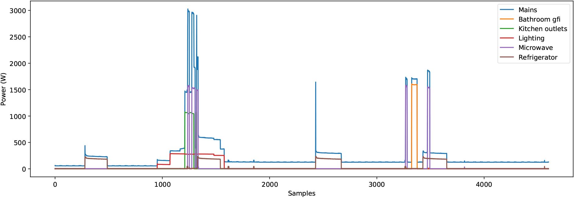
Figure 1.
REDD sample of the power consumption of different household appliances and the aggregated consumption.
Several approaches [37, 38, 39] use the CWT and scalograms applied to NILM to detect two new features that help identify the appliance: Centroid and boundary points of the CWT. The main difference from our approach is that they use the scalogram to detect a feature. Still, we process the entire scalogram using CNNs to detect and classify the operating appliances.
In summary, many studies address the problem of detecting and classifying household appliances according to their energy consumption. As mentioned above, several machine learning techniques have been applied to achieve this goal, including deep learning architectures, and satisfactory results have been obtained. On the other hand, numerous works on detection or classification use scalograms generated from the data. This type of data transformation has been applied in other domains, but to the best of our knowledge, it has not been applied to the problem of home appliance detection. Another difference between our approach and the state-of-the-art is the comparison of machine learning techniques with and without data augmentation, which shows the strong influence of data augmentation.
3.Materials and methods
In this section, we present the dataset and the methodology proposed for the experimental study. First, we will analyze the content and characteristics of the dataset we have been working on. Finally, the experimental framework is described step by step along with the procedure followed.
All experiments were carried out on a machine equipped with a 4.35 GHz AMD Ryzen 7 3700x CPU, 32GB of DDR4 3200 RAM, and an NVIDIA GeForce 3080 graphics card with 10GB of GDDR6X memory. Python 3.9 has been used to perform all the experiments, and among the libraries used, we can find: scikit-learn, for machine learning functions; scaleogram, for the generation of the scalograms; and matplotlib, for the creation of the graphs. The source code used in this study is available in the GitHub repository [40]. The repository contains implementations of the machine learning models used as well as the datasets used in our experiments.
3.1REDD dataset
For this work, we have selected the Reference Energy Disaggregation Data Set (REDD) [19]. The dataset contains 24 hours power consumption data from six residential buildings in the United States with a total duration of 119 days. The dataset contains the house’s total power consumption, that is, with the sum of the appliances (aggregated consumption) and the consumption of each appliance separately (disaggregated consumption). The measurements consist of two types of data sampling frequencies. The mains data are recorded at a sampling period of 1 second, while the appliances’ measurements are taken at a sampling period of 3 seconds. Additionally, high-frequency current and voltage measurements are available, sampled at a frequency of 15 kHz. Figure 1 shows the sample data we will work with. The graph represents the energy consumption (y-axis) of different appliances over time (x-axis). As seen, the “Mains” time series represents the aggregate energy. In contrast, multiple series shows the power consumption of different appliances, such as the washing machine, the dishwasher, or the microwave.
An approach to evaluating the performance of a machine learning model on a dataset with a limited number of observations is to use cross-validation. This study used a six-fold cross-validation (one per house) to consider each house as a test split and improve the model’s generalizability. To perform cross-validation, the dataset was divided into six equal folds. In each cross-validation iteration, one of the six houses was used as the test set, and the other five houses were used as the training set.
The model was trained in the training set with five houses and its performance in the test set was evaluated. We repeated this process six times, each with a different house held as the test set.
Using a 6-fold cross-validation, we obtained an estimate of the model’s generalization performance on the entire dataset. This approach allowed us to evaluate the performance of the model in each individual house as well as the overall performance in all six houses.
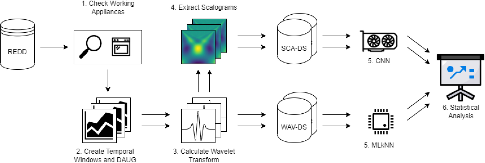
Figure 2.
Summary representation of the methodology followed. The arrows indicate the number of datasets passed to the next step. Two arrows indicate when the step produces a result with and without data augmentation.
To carry out the experiments, different transformations were made to the dataset. These transformations are detailed in the following section (Section 3.2).
3.2Methodology
This section develops the methodology used to carry out the study. Starting from the dataset documented in Section 3.1, in order to obtain the datasets on which to work and thus apply machine learning techniques, some transformations have been applied and are summarized in Fig. 2.
As shown in Fig. 2, the methodology consists of the following six steps: First, based on the REDD data set, it is necessary to check and verify which devices are working at any given time (1). Second, the data are divided into sliding temporal windows to improve data processing, with a window size of 600 samples and a temporal shift of 200 samples. In this step, we also apply a data augmentation algorithm to enhance the dataset. From this step, we start working in parallel with the original data and the data with data augmentation (DAUG) (2); in the third place, the Continuous Wavelet Transform (CWT) is computed for each time window, and the wavelet dataset (WAV-DS) is built (3); in the fourth place, the scalograms are extracted from the CWT of the previous step, and with this set of images, the scalogram dataset (SCA-DS) is built (4). In the fifth step, the machine learning method (MLkNN) and the deep learning method (CNN) are applied to the generated datasets (5 and 6). Finally, the results are discussed, and a statistical analysis is performed. It should be noted that when the methodology starts working with the original data set and with those with data augmentation, it is illustrated in Fig. 2 with two arrows.
3.2.1Data preprocessing
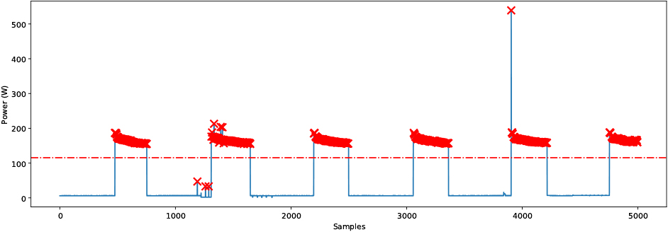
As mentioned above, the methodology starts with REDD. The first step is to check which appliances are working at any given time. Considering that REDD has aggregated and disaggregated data, it is possible to know at any moment in time which appliance is working. Therefore, using the disaggregated datasets, a threshold value is calculated by which we will know whether the appliance is active or not. Therefore, a threshold value was calculated for each household appliance to confirm that it is working at that moment and therefore use this as a binary class. To achieve this, the threshold was calculated based on the mean value of the consumption peaks and adjusted for a bias error of 30%. In other words, the consumption peaks of these appliances were calculated and if their value exceeded the threshold, it was confirmed that this appliance was activated. In Fig. 3 we can see an example of the calculation of this threshold for the refrigerator case. Here, we can see an extract of the refrigerator’s consumption and those consumption peaks derived from this appliance marked in red. Furthermore, we can see a horizontal line in the graph that represents the threshold calculated by which we will define whether the refrigerator is working. In this way, the refrigerator operates when the consumption of the refrigerator is above this threshold.
Figure 3.
Bias threshold calculation sample for the refrigerator.
Once we have identified when each device operates in the time series, we move on to the next step: generating the time series window. This study aims to identify which devices are working within a time period, and in this step we define the time-space window with which we will work. After several tests focusing on the system’s usability for the end user, it was concluded that a time window of 600 seconds with a shift of 200 samples would be optimal. By analyzing the data, we observed that certain devices tended to operate in at specific time intervals. For example, some appliances have recurring patterns of activity every 10 minutes such as the refrigerator. Therefore, by setting a time window of 600 seconds (10 minutes) and a shift of 200 samples, we could effectively capture the operating patterns of such devices. A time window of 600 seconds allows us to examine a sufficiently long duration to identify recurring activity patterns and to extract meaningful insights from the data. The shift of 200 samples ensures that we capture overlapping segments within the time window, which allows us to detect the activity of devices in adjacent intervals. Through iterative testing and analysis, we found that this configuration provided a good balance between capturing device performance at the desired interval. It allowed to effectively identify and monitor devices operating at 10-minute intervals, which is valuable information to understand energy consumption patterns and making informed decisions. Next, we divide our entire dataset into 10-minute intervals where we know which devices are running at that time.
3.2.2Data augmentation
In this step, the data augmentation algorithm is applied. As mentioned in Section 1, one of the key findings of this study is the improvement of the models by using data augmentation to identify applications by power consumption. New windows, including new appliance uses, were added to the original time-series window dataset to perform data augmentation. In other words, new windows were created in which different appliances were aggregated.
The idea is to increase the frequency of the appearance of household appliances. To this end, new windows have been created based on the disaggregated consumption of each household appliance. For each window of our training set, we disaggregate the consumption of each appliance and select another random window from that set as the target. Given the disaggregated consumption and the window of another random time, both energy consumptions are aggregated, thus generating a new window with the same appliance but in a new situation. In this way, the data of each appliance is augmented, allowing the network to identify it with other appliances that may hinder its detection. The proposed data augmentation method is also detailed on Pseudo-Code 1.
: Pseudo-code of Energy-Based Data Augmentation.[1] min_augmentations: minimum number of augmentations per label. max_occurrences: maximum number of occurrences per label not to apply data augmentation. windows_per_label
annotations
label, daug_factor in daug_factors window, appliances, _, _ in annotations appliance in appliances meter
annotations
Table 1
Number of samples used in the two different types of datasets. The quantity of samples after DAUG corresponds to the maximum number of augmented samples per house. The DAUG Factor column indicates the factor of data augmentation applied to each appliance. In bold are the labels that will be used to evaluate the models
| Appliance | # Samples | After DAUG | DAUG factor |
|---|---|---|---|
| air_conditioning | 330 | 9,630 | 10 |
| bathroom_gfi | 216 | 4,479 | 14 |
| dishwasher | 169 | 4,284 | 18 |
| disposal | 57 | 3,260 | 53 |
| electric_heat | 44 | 6,116 | 69 |
| electronics | 220 | 4,401 | 14 |
| furnace | 577 | 7,321 | 6 |
| kitchen_outlets | 469 | 6,615 | 7 |
| lighting | 2,710 | 25,431 | 2 |
| microwave | 527 | 6,589 | 6 |
| miscellaneous | 6 | 3,006 | 500 |
| none | 1,894 | 1,894 | 0 |
| outlets_unknown | 529 | 7,917 | 6 |
| oven | 54 | 6,102 | 56 |
| refrigerator | 6,273 | 44,120 | 1 |
| smoke_alarms | 6 | 3,026 | 500 |
| stove | 98 | 3,518 | 31 |
| subpanel | 88 | 5,128 | 35 |
| washer_dryer | 258 | 6,643 | 12 |
In this way, new windows are created, including situations where one or more appliances operate simultaneously. At the end of this step, we will work with two sets of time series: one containing the original REDD data and a second set of time series containing data generated by the data augmentation algorithm (DAUG).
Table 1 shows the number of examples we have obtained for each appliance. The number of samples in the “# Samples” column indicates the number of samples containing the data in which the appliance operates. The column “After DAUG” shows the maximum number of samples after applying the data augmentation. Since data augmentation uses random windows in the training set, some appliances have more presence than others. However, since this selection of windows is random, the number of samples per appliance in each run will vary. Therefore, the maximum number obtained from each appliance is shown. This is the maximum contemplated and may be slightly lower due to some iterations due to the random selection of windows during data augmentation. The “DAUG Factor” column indicates the factor of data augmentation. A factor of “1” indicates that a new sample is created for each original sample.
As appliances may appear in windows of data augmentation that contain other appliances, it is possible that the data augmentation factor may not correspond to the maximum number of samples generated. This happens because when we increase an appliance, for example, “microwave”, we have to add it to a new random window containing other appliances, for example, a window with the appliances “refrigerator” and “oven”. Therefore, even if we do not want to increase the “refrigerator” anymore directly, it appears again through the newly created window. Consequently, although the refrigerator increase factor is “1” and this should correspond to 12,546 instances, 44,120 samples have been counted, with a difference of 31,574 samples resulting from the occurrence of increases in other appliances. This allows the model to learn from appliances such as microwaves alongside more common appliances such as refrigerators and less common appliances such as ovens.
As can be seen, there is a large variability in the data between appliances, where we can see that appliances such as the smoke alarm have only 6 scalograms. On the contrary, we have 6,273 samples from the refrigerator. This situation occurs because we are using real data. Therefore, we use appliances that are used 24 hours a day and others that consume only energy when necessary, such as the smoke detector. Considering that there are certain appliances for which there are not enough data available, data augmentation (DAUG) techniques have been applied to work with a sufficient dataset. Therefore, at this point, the study is carried out taking into account these two different types of datasets: the first one, in which deep learning techniques are applied to the transformation calculated based on the initial data; and a second type of dataset in which, in addition to the initial data, also includes the augmented data from the DAUG algorithm. However, not all the appliances listed will be used in the experiments because the six houses used do not have all of them. Therefore, we will keep only the appliances that have at least, for each fold, five samples on test and also contain that label on training. These appliances are in bold in Table 1.
Table 2
Mean consumption per appliance in the different houses. The presented value corresponds to the mean consumption in watts of the appliances when they are considered active. In bold are the labels that will be used to evaluate the models
| Appliance | House 1 | House 2 | House 3 | House 4 | House 5 | House 6 |
|---|---|---|---|---|---|---|
| air_conditioning | 974.39 | |||||
| bathroom_gfi | 1,606.44 | 1,275.04 | 1,146.83 | 1,610.10 | 946.04 | |
| dishwaser | 1,072.46 | 1,198.56 | 736.86 | 1,317.63 | 1,249.69 | |
| disposal | 394.29 | 358.26 | ||||
| electric_heat | 804.79 | 444.31 | ||||
| electronics | 210.89 | 242.14 | 486.92 | |||
| furance | 679.45 | 594.26 | 652.96 | |||
| kitchen_outlets | 1,522.48 | 1,054.50 | 755.18 | 516.46 | ||
| lighting | 152.29 | 191.23 | 141.57 | 393.74 | 125.53 | |
| microwave | 1,519.50 | 1,836.58 | 1,712.79 | |||
| miscellaeneous | 41.00 | |||||
| outlets_unknown | 121.15 | 79.50 | 201.19 | |||
| oven | 2,051.95 | |||||
| refrigerator | 201.07 | 171.52 | 128.82 | 173.47 | 148.93 | |
| smoke_alarms | 44.00 | 29.00 | ||||
| stove | 1,502.10 | 1,671.89 | ||||
| subpanel | 265.32 | |||||
| washer_dryer | 2,700.21 | 2,519.77 | 784.81 |
The DAUG function combines disaggregated consumption and the total consumption of other intervals, thus generating new wavelets with different overlaps of appliances. In addition, to add more variety, random time shifts are performed, adding more variety to the augmented data. Table 1 in the column “After DAUG” shows the total number of examples available after data augmentation.
We established a minimum number of 3,000 instances per appliance to perform data augmentation, thus ensuring a minimum amount for a proper training process. However, this number may increase due to the accumulation of other appliances as they appear in other windows during their generation.
As can be seen, much more data is now available. We can see how we have gone from having 169 dishwasher scalograms to having 4,479, or from having 57 examples where the disposal was used to having 3,260. At this point, we could consider that we have enough data for the Deep Learning algorithms in the second scenario to obtain better results.
Table 2 presents the mean consumption obtained in Watts for the different household appliances. It is important to recognize that households may differ in terms of the appliances they have. Among the available appliances, the most prevalent are “bathroom_gfi”, “dishwaser”, “lighting” and “refrigerator”, which are found in five out of six homes. Furthermore, it can be observed that there are some appliances that have a lower consumption compared to others, such as the “refrigerator”, with a mean consumption of 164.76 W, which has a much lower consumption than, for example, “bathroom_gfi”, with a mean consumption of 1316.89 W.
In summary, we have two different scenarios. In each scenario, we have two different types of dataset, that is, first, we have a scenario in which we will work with the wavelet transformed data (WAV-DS); and a second scenario in which we will work with the scalograms extracted from these wavelet transforms (SCA-DS). In each of these scenarios, we have worked with two datasets on each: one in which we work with the original data, which is composed of 8,972 instances; and a second dataset which includes the data augmentation in which a maximum of 58,031 instances are used.
3.2.3Wavelet and scalogram transformations
Once we have the sets of time intervals, we apply the CWT [41] to the data. The CWT is a signal processing technique that uses a wavelet function to analyze signals in the time-frequency domain. This allows for identifying features in the signal that change over time and can provide valuable information about the signal’s properties.
The wavelet is shifted and scaled to analyze the signal at various positions and scales to compare the signal. Scaling is accomplished by dilating or compressing the wavelet, which is equivalent to modifying its width, and shifting refers to moving the wavelet along the signal. The CWT produces a function of two variables, known as the wavelet coefficient function, by comparing the signal to the wavelet at various scales and positions. Figure 4 shows an example of the convolution undergone by an example interval of the time series with the Morlet wavelet.
Figure 4.
Example of consumption signal (a), wavelet with a width of 1 and frequency of 2 (b), and the convolution of the selected wavelet with the signal (c).
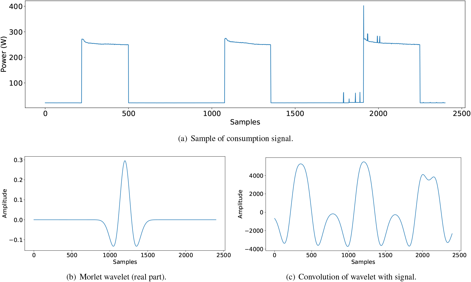
Figure 5.
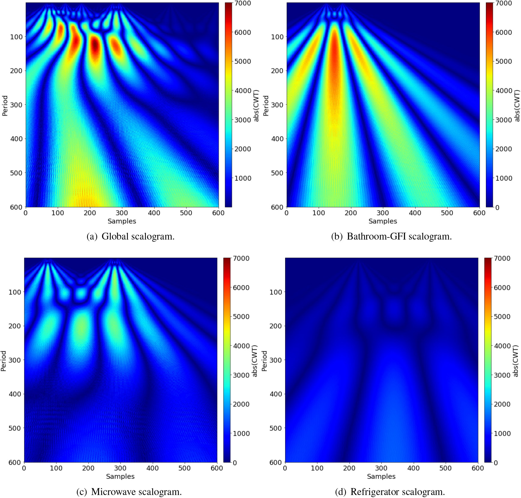
Scalograms generated from a window with a) the consumption of three appliances (bathroom-gfi, microwave, and refrigerator); b) the disaggregated consumption of bathroom-gfi appliance; c) the disaggregated consumption of microwave appliance; d) the disaggregated consumption of refrigerator appliance.
The wavelet coefficient function obtained from the CWT provides a detailed representation of the signal frequency content at different scales and positions, making it a powerful tool for signal analysis. It can be used to identify and characterize different patterns or structures within the signal that are not easily observable using other methods. The CWT is a valuable technique for analyzing signals with complex frequency content and temporal dynamics.
In the present work, it has been used to decompose the power consumption signal from each house into different time and frequency scales, which would help identify specific patterns and trends in power consumption over time. In this way, we will go from having time series intervals to wavelet transforms. As mentioned above, WAV-DS is built with a set of wavelet transforms. It is worth recalling that after executing this step, we will obtain WAV-DS without and with DAUG.
Finally, once we have our sets of wavelet transforms (without and with DAUG), the fourth part of the methodology is reached. In this case, the scalograms are extracted for each wavelet transform by using pywavelets library [42]. A scalogram is a graphical representation of the results of the continuous wavelet transform. It is a two-dimensional graph that displays the wavelet coefficient function, which provides information about the signal’s frequency content at different scales and positions. The x-axis of the scalogram represents the time and the y-axis represents the wavelet scale used for the analysis. The intensity of the color or shading of each point in the plot corresponds to the amplitude of the wavelet coefficient function, which provides information about the signal’s energy at a particular scale and time.
In this way, it is possible to build a dataset composed of a set of images that are the WAV-DS scalograms. In this work, the scalograms have been used to visualize the patterns and trends in the power consumption data for each time interval and to be able to use these images to apply Deep Learning techniques and perform comparisons between the different techniques. Figure 5 shows different examples of scalograms in the same window with total and disaggregated consumption of appliances in house 1.
Therefore, we go from having a dataset composed of time series of the aggregate power consumption to having a set of wavelet transforms (WAV-DS) and scalograms from those wavelets (SCA-DS) of 10-minute time windows. It should be noted that, for each of these datasets, we will work with the versions without and with DAUG.
3.2.4Classification models
The next step of the methodology (Step 5 in Fig. 2) is given by applying two different classification algorithms. On the one hand, we will use the MLkNN algorithm. MLkNN is a classification algorithm used for multi-label classification problems [43], which is necessary for this problem, as more than one appliance may appear in the same time window. The algorithm is based on the K-Nearest Neighbor (KNN) method and uses a supervised learning technique to assign labels to new instances. The main goal is that for each data instance, the K-Nearest Neighbors of it in the feature space are searched, and their labels are used to assign a label to the current instance. The labels are considered as binary vectors, where each label represents a distinct class. The algorithm aims to find the k nearest neighbors in the feature space and assign labels based on the majority voting of the labels from the neighbors. In addition, this algorithm has been chosen because it is one of the most widely used in the literature [44, 45, 46]. This algorithm works with numerical data, so, in our study, we have used as input the WAV-DS composed of the wavelets extracted from the data and discussed in the previous Section.
On the other hand, we will use one of the most widely used Deep Learning techniques, such as the classification architecture based on Convolutional Neural Networks (CNN), and more specifically the ResNet-50 architecture [47]. ResNet-50 is a deep convolutional neural network (CNN) architecture commonly used for image recognition tasks. This architecture uses a technique called “residual connection” to allow the network to learn deeper representations of images. A residual connection is a way to allow information to flow directly through a layer without additional processing. This helps avoid the problem of gradient fading, which can make it challenging to train very deep neural networks. ResNet-50 consists of 50 layers including convolutional layers, pooling layers, and fully connected layers. Specifically, the ResNet-50 architecture comprises five stages, each with a different number of residual blocks. The number of layers in each stage is as follows:
• Stage 1: 1 convolutional layer
• Stage 2: 3 residual blocks, each containing 3 convolutional layers
• Stage 3: 4 residual blocks, each containing 4 convolutional layers
• Stage 4: 6 residual blocks, each containing 6 convolutional layers
• Stage 5: 3 residual blocks, each containing 3 convolutional layers
In this study, ResNet-50 is used to classify multiple categories of appliances from the sliding window scalogram, detailed in Section 3.2.
The Binary Cross Entropy (BCE) loss with an initial sigmoid function was selected to implement this multicategory problem on ResNet-50. BCE is a commonly used loss function in machine learning for binary classification problems, such as the appearance or non-appearance of a household appliance. This loss measures the difference between the predicted probability distribution and the true probability distribution. Nevertheless, the BCE loss must be modified to handle one-hot-encoded vectors when dealing with multicategory classification problems, where the output has more than two possible classes, such as the appearance of multiple household appliances. The output of this network consists of the probability distribution for each class as a vector. To obtain a binary classification for each class, an activation threshold of 0.5 was established, as this presents a correct detection ratio. However, this value could be modified to reduce false positives at the cost of losing true positives if necessary.
The experiment was carried out following the cross-validation method, where the selected folds correspond to the six houses of the REDD dataset. Hence, six experiments were carried out for each model with the combination of use and non-use of augmentations. Each fold uses as training the rest of the houses available for training and the one selected as validation.
The results shown in this study correspond to the mean and standard deviation obtained over all the folds, considering only labels with at least five samples in their test set. The labels that meet this support are bathroom_gfi, dishwasher, disposal, electronics, furnace, kitchen_outlets, lighting, microwave, outlets_unknown, refrigerator, and washer_dryer.
Therefore, the MLkNN algorithm will work with WAV-DS; on the other hand, CNN will process SCA-DS. It should be noted that each algorithm will use its corresponding dataset with the original data and another with the data after applying the data augmentation algorithm.
As a last step, comparative tables will be shown and the results will be discussed in Section 4.
Table 3
MLkNN results for WAV-DS regarding precision, recall, F1-score, and support for each appliance. The highest F1-score for each appliance is in bold
| Normal | DAUG | |||||||
|---|---|---|---|---|---|---|---|---|
| Appliance | Precision | Recall | F1-score | Precision | Recall | F1-score | Support | |
| bathroom_gfi | 0.19 | 0.11 | 0.13 | 0.22 | 0.22 |
0.19 | 53.250 | |
| dishwasher | 0.31 | 0.51 | 0.36 | 0.43 | 0.55 |
0.480 | 33.800 | |
| disposal | 0.05 | 0.02 |
0.03 | 0.00 | 0.00 | 0.00 | 28.500 | |
| electronics | 0.16 | 0.03 | 0.05 | 0.37 | 0.19 |
0.25 | 181.000 | |
| furnace | 0.42 | 0.183 | 0.26 | 0.46 | 0.50 |
0.48 | 120.000 | |
| kitchen_outlets | 0.12 | 0.09 | 0.16 | 0.23 | 0.16 |
0.18 | 74.667 | |
| lighting | 0.48 | 0.68 |
0.52 | 0.42 | 0.63 | 0.45 | 356.167 | |
| microwave | 0.48 | 0.17 | 0.22 | 0.77 | 0.38 |
0.49 | 175.667 | |
| outlets_unknown | 0.13 | 0.33 |
0.19 | 0.07 | 0.29 | 0.10 | 82.000 | |
| refrigerator | 0.94 | 0.62 | 0.72 | 0.96 | 0.63 |
0.76 | 1254.600 | |
| washer_dryer | 0.31 | 0.09 | 0.14 | 0.64 | 0.09 |
0.16 | 59.000 | |
3.2.5Statistical tests
To verify the performance of the different algorithms proposed, a statistical framework has been applied in two steps: Friedman’s statistical test and Holm post-hoc procedure. The Friedman test is a non-parametric test used to compare the effects of several conditions or treatments on an ordinal dependent variable. The purpose of the test is to determine whether there are significant differences between the treatments evaluated, such as the methods in our study [48] i.e., if at least one of them has a different effect than the others. If the null hypothesis is rejected, it can be concluded that at least one treatment is different from the others. Once the Friedman test is performed and the null hypothesis is rejected, a post-hoc procedure is applied to determine which treatments are significantly different from each other. In this case, the Holm post-hoc procedure will be used [49]. The Holm post-hoc procedure is a correction for multiple comparisons that is used to adjust the
In summary, the Friedman test is going to be used to determine if there are significant differences between the evaluated algorithms, while the Holm post-hoc procedure is used to determine which methods are significantly different from each other after the null hypothesis has been rejected.
4.Results and discussion
This section details the results after applying the methodology developed in the previous section. This section is divided into two sections: first, the results of applying the MLkNN algorithm to the original data and the augmented data are presented (Section 4.1); and second, the results of using ResNet-50 on both data sets are shown (Section 4.2). Then, a statistical test will be applied and the results obtained in both models will be discussed.
Table 4
CNN results for SCA-DS without data augmentation regarding precision, recall, F1-score, and support for each appliance. The highest F1-score for each appliance is in bold
| Normal | DAUG | |||||||
|---|---|---|---|---|---|---|---|---|
| Appliance | Precision | Recall | F1-score | Precision | Recall | F1-score | Support | |
| bathroom_gfi | 0.12 | 0.07 | 0.05 | 0.36 | 0.38 |
0.35 | 53.250 | |
| dishwasher | 0.10 | 0.02 | 0.03 | 0.38 | 0.52 |
0.42 | 33.800 | |
| disposal | 0.00 | 0.00 | 0.00 | 0.35 | 0.23 |
0.27 | 28.500 | |
| electronics | 0.00 | 0.00 | 0.00 | 0.28 | 0.41 |
0.33 | 181.000 | |
| furnace | 0.76 | 0.35 | 0.48 | 0.61 | 0.69 |
0.65 | 120.000 | |
| kitchen_outlets | 0.32 | 0.15 | 0.16 | 0.53 | 0.61 |
0.55 | 74.667 | |
| lighting | 0.47 | 0.61 |
0.49 | 0.34 | 0.64 | 0.40 | 356.167 | |
| microwave | 0.41 | 0.17 | 0.18 | 0.74 | 0.63 |
0.65 | 175.667 | |
| outlets_unknown | 0.07 | 0.09 | 0.08 | 0.16 | 0.26 |
0.19 | 82.000 | |
| refrigerator | 0.90 | 0.75 | 0.81 | 0.92 | 0.82 |
0.86 | 1254.600 | |
| washer_dryer | 0.59 | 0.39 | 0.47 | 0.66 | 0.65 |
0.65 | 59.000 | |
4.1MLkNN results
The results after applying MLkNN to the two data sets are presented in this section. The same cross-validation was applied for both datasets, with the results presented being the mean metric for all folds. In addition, Grid Search CV has been used to optimize the parameters, taking the number of neighbors (
Table 3 shows the MLkNN results regarding precision, recall, F1-Score, and support for each appliance, for both the normal dataset and DAUG. The results are the mean values of the validation for all the houses; therefore, the mean is shown together with the standard deviation for each value. Additionally, the values in bold indicate the highest F1-Score for each appliance. Precision measures how many of the predicted positive cases are actually true positives, while recall is calculated as the ratio of true positives to the sum of true positives and false negatives. The F1-Score is a harmonic mean between precision and recall. Support refers to the mean number of cases in the test split per fold.
In this case, the results show that the models perform poorly for most labels. It can be seen that no F1-score higher than 0.5 is achieved for all appliances except the refrigerator and lighting, where 0.76 and 0.52, in DAUG and normal, respectively, are achieved. Furthermore, it should be noted that the refrigerator label has a precision of 94.2 and 96.4 in both models, suggesting that the model can effectively identify this class. Furthermore, we can see that the microwave has also achieved proper precision, reaching 77.3 in the DAUG model, from 48 without data augmentation. However, there are appliances whose prediction has not been good, as is the case of outlets_unknown, which has obtained a precision of 0.13 and 0.65 in each model. Unfortunately, we did not find a reasonable explanation as to why for this appliance, compared to the rest, the models obtain results that can be significantly improved.
4.2CNN results
This Section presents the results of CNN. In this case, the scalograms generated from the wavelets were used as data to train the model. The results are presented for SCA-DS without and with data augmentation (DAUG). The Resnet-50 architecture and a fine-tuning with the same configuration for both datasets: 4 epochs with frozen weights and 20 epochs with unfrozen weights, and a base learning rate of 0.003. The results of these models are shown in Table 4. As in Table 3, the best result in terms of F1-score for each appliance is shown in bold.
As can be seen, the results obtained by the CNN applied to the scalograms have obtained good results. We can see how, in terms of F1-Score, the highest values are in the model that has used data augmentation. It should be noted that the furnace, the kitchen_outlet, the microwave, the refrigerator, and the washer_dryer obtained F1-Score above 0.5, with the fridge the highest with 0.864 for DAUG. This means that the model has identified some positive examples for this class, but has missed many others, resulting in low recall.
In this table, we can see that the algorithm has improved significantly in terms of precision, recall, and F1-Score for most of the labels compared to the results of MLkNN. In particular, the CNN-DAUG method has significantly improved the classification of disposal, kitchen_outlets, and washer_dryer appliances, which were difficult to classify in MLkNN, even with data augmentation.
In addition, it has improved the recall and precision of the washer_dryer and furnace appliances. In particular, the classification of the washer_dryer label stands out, with a much higher recall value compared to MLkNN, achieving an improvement of
The results indicate that the CNN model with the proposed data augmentation has achieved significantly better performance in classifying most appliances than the MLkNN model. However, the most significant change is in data augmentation, which has led to detections where previously this was not possible.
As can be seen, there has been a notable improvement in the use of data augmentation, in general, in all household appliances. It can be seen that the disposal and electronics have obtained an F1-Score of 0.269 and 0.333 respectively, while in the SCA-DS without DAUG, they obtained 0.0. Furthermore, we can see that in the case of the kitchen_outlets and microwave, the result has improved significantly, achieving a gain in F1-Score of
Finally, we compare the results obtained with MLkNN and CNNs with and without data augmentation in Fig. 6. The figure illustrates the results for each algorithm in terms of the F1-Score for the appliances.
Focusing on the MLkNN results, it can be seen at a glance that the MLkNN-DAUG results generally improve MLkNN. However, if we analyze the details, it can be observed that the result of some appliances was better in MLkNN. On the one hand, we find appliances where the results between the two models are similar, like lighting and washer_dryer. There are other cases in which the DAUG has had a slight negative influence, such as in the case of outlets_unknown. We also found other appliances whose identification has been facilitated by the DAUG, such as electronics, furnaces, dishwashers, and microwaves. It could be affirmed that, in general, DAUG has helped identify the appliances, as the results are improved in 8 of the 11 appliances shown. Moreover, the improvement is very noticeable in
Figure 6.
Comparative between CNN and MLkNN F1-Scores for the appliances with and without data augmentation.
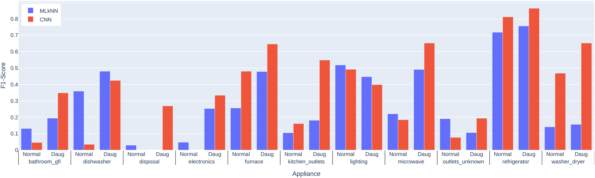
some cases, such as those with high consumption, such as in the furnace or the microwave. However, some appliances, such as lighting, do not improve with DAUG, and this may be due to the fact that the consumption of this one has a shape that could lead to confusion with others.
It was observed that the “refrigerator” label had the best results in all algorithms evaluated. In contrast, the labels “dishwasher” and “microwave” presented the lowest performance, and this could be because these techniques do not perform well in minority classes, since classes with a more significant amount of real data will exhibit better predictive performance. In general, it can be concluded that classifying electrical appliances in a smart home remains a challenge for machine learning algorithms. The results suggest that the choice of algorithm is highly dependent on the classification label considered and that further exploration and experimentation with different machine learning techniques are still needed to improve the performance of appliance classification in a smart home.
The results indicate that the CNN and CNN-DAUG algorithms achieved the best results for most appliances, with F1-Scores that reach 0.86 in the refrigerator. In contrast, the MLkNN and MLkNN-DAUG algorithms had lower performance, especially in detecting appliances such as disposal, kitchen_outlets, and washer_dryer. It is important to note that the results presented may depend on various factors, such as the quality and quantity of training data, the selection of features, and the parameters used in classification algorithms. In addition, a statistical evaluation would be of interest to determine whether the differences between the algorithms are significant. In general, the results suggest that using convolutional neural networks (CNN) with the proposed data augmentation can effectively detect home appliances, obtaining more significant results in minority classes.
4.3Statistical analysis
This section presents the results of the statistical analysis. To carry out the statistical test, the mean F1-Score of the appliances for each MLkNN and CNN was taken into account, without and with data augmentation. To determine whether these performance differences were statistically significant, the non-parametric Friedman test and the Holm post hoc test were used to determine any significant differences between the performances of multiple results. The test uses a chi-square distribution to calculate a
Table 5
Sorted ranked mean for Friedman’s test
| Algorithm | Ranking |
|---|---|
| CNN-DAUG | 2.48 |
| MLkNN-DAUG | 4.54 |
| MLkNN | 5.45 |
| CNN | 5.70 |
Table 6
Post-hoc Holm procedure results using CNN-DAUG as the control method
| Algorithm |
|
|
|---|---|---|
| MLkNN-DAUG | 0.0389 | 2.0643 |
| MLkNN | 0.0059 | 2.9726 |
| CNN | 0.0038 | 3.2203 |
According to the Friedman test and the mean ranking in Table 5, CNN-DAUG is the best algorithm, followed by MLkNN-DAUG and MLkNN, and CNN in the last position. Furthermore, according to Holm’s post hoc test (Table 6), there are significant differences between CNN-DAUG and the other algorithms, as the
4.4Comparison with state-of-the-art
In this section, we will compare the performance of our proposed algorithms with the current state-of-the-art methods in the field. We will consider a wide range of popular and well-established techniques as benchmarks to ensure a fair and comprehensive comparison. These methods will be evaluated using the same dataset and performance metrics used for our algorithms. This will ensure that the comparison is based on the same ground and hence, provide a reliable assessment of the performance of our proposed approaches.
Nevertheless, some state-of-the-art studies do not sufficiently specify the partitions established and the data treatment performed. For this reason, when they do not determine the house used as validation, we compare them with the average obtained by all the houses, which will be specified in the description of the results.
In contrast to Machlev et al. [22], our study focuses on all available appliances, validating with 11 due to the number of sample restrictions. Nonetheless, we have used the four appliances that overlap with their research for this comparison. To establish a basis, we utilized the first scenario, household two. This was deemed appropriate since other scenarios do not encompass the entirety of electricity usage in a household or use different datasets.
Table 7 reveals a significant improvement in the classification of “dishwasher”, with a gain of
Table 7
Comparison of F1-Score over four appliances on House 2 between Machlev et al. [22] and our proposed method
| Appliance | Machlev et al. | Our |
|---|---|---|
| Dishwasher | 0.36 | 0.55 |
| Kitchen Outlet | 0.72 | 0.79 |
| Refrigerator | 0.98 | 0.97 |
| Microwave | 0.77 | 0.72 |
Our next step was to compare our results with those from the studies by Singh et al. [23], and Verma et al. [24]. Although these studies did not present the validation data, we assumed they evaluated a random selection, given that they only indicated the percentage used. We used the average obtained in our experiments to compare our results, validated using independent houses. We also included the standard deviation of these results. As in the previous study, we compared the coinciding ones as they do not have many classes.
Table 8 compares our proposed algorithms’ performance with existing studies, where “dishwasher”, “Kitchen Outlet” and “Lighting” show inferior results. The “Washer Dryer” scores similarly, considering the standard deviation, while our proposal demonstrates superior outcomes in the “refrigerator” category, with a gain of
Table 8
Comparison of F1-Score over five appliances between Singh et al. [23], Verma et al. [24] and our proposed method
| Appliance | Singh et al. | Verma et al. | Our |
|---|---|---|---|
| Dishwasher | 0.74 | – | 0.43 |
| Kitchen outlet | 0.66 | 0.76 | 0.55 |
| Lighting | 0.70 | 0.72 | 0.40 |
| Washer dryer | 0.70 | 0.74 | 0.65 |
| Refrigerator | – | 0.76 | 0.86 |
We compared our study with the one by Hur et al. [25], which had two similar appliances. Their study included House 1 and House 3, training with one and validating with the other. However, their model could result in low generalization when applied to an actual system. To avoid this, our training data included the remaining houses, even if this means a deterioration in performance.
Table 9 displays the outcomes obtained from testing the “refrigerator” and “microwave” appliances in two houses, comparing the study of Hur et al. [25] and ours. It is noticeable that the “refrigerator” results are lower in House 1, possibly due to differences in consumption patterns compared to the other houses. However, compared to Hur et al.’s study, our “refrigerator” results in House 3 show an improvement of
Table 9
Comparison of F1-Score over two appliances on House 1 and House 3 between Hur et al. [25] and our proposed method
| Hur et al. | Our | |||
|---|---|---|---|---|
| Appliance | H.1 | H.3 | H.1 | H.3 |
| Refrigerator | 0.84 | 0.85 | 0.46 | 0.97 |
| Microwave | 0.81 | 0.82 | 0.60 | 0.64 |
Finally, we compared our results with the most recent study presented, which, like us, utilizes 2D-CNN models and wavelets, thereby giving a more direct comparison standpoint. In their research, Shahab et al. [26] used four appliances to test their system, for which we will provide comparative results. Furthermore, in this case, the metric used is accuracy, as they used it in their study to showcase their per-appliance results.
Table 10 shows the average accuracy obtained in our study with different houses, accompanied by standard deviation, compared to the study by Shahab et al. [26]. As their research does not specify which houses were used for training and testing, we assume that the partition selection is random over the entire set. Based on these results, we can see that our system surpasses the accuracy obtained in the “Dish Washer” class with an improvement of
Table 10
Comparison of accuracy over four appliances between Shahab et al. [26] and our proposed method
| Appliance | Shahab et al. | Our |
|---|---|---|
| Dish washer | 94.60% | 97.76% |
| Microwave | 94.41% | 94.09% |
| Refrigerator | 86.58% | 81.71% |
| Washer dryer | 89.97% | 98.95% |
5.Conclusions
In this study, we have conducted a thorough evaluation of two machine learning algorithms, MLKnn and CNN, in the context of appliance classification within a smart home environment. Our analysis focused on comparing these algorithms in terms of precision, recall, and F1-Score using both an original dataset and one augmented with data augmentation techniques. The results have clearly demonstrated that the CNN model, particularly when enhanced with our proposed data augmentation techniques, exhibits superior performance over MLKnn in handling the complexities of NILM tasks. This combination of advanced modeling with customized data enhancement represents a significant advancement in the classification of electrical appliances, effectively addressing both the challenges of data scarcity and the variability inherent in appliance energy usage patterns.
However, while our findings indicate a notable improvement, we also observed that the classification metrics for many appliances did not reach the high standards anticipated. This highlights a critical aspect of our research, showcasing the intricate challenges inherent in NILM due to the diverse and variable nature of appliance behavior and energy consumption patterns. These results underscore the need for the ongoing refinement and development of more sophisticated models and approaches in this domain.
In addition, the practical implications of our study are significant. The deployment of our system in homes or buildings with access to real-time electrical consumption data, facilitated by low-cost sensors or smart meters, opens up possibilities for detailed energy use analysis. This could lead to substantial reductions in energy waste, lower energy bills, and a decrease in greenhouse gas emissions, contributing to environmental sustainability.
Future research directions, as identified from our study, include exploring diverse data preprocessing techniques to enhance the quality of input data and further deepening the investigation into the impact of data augmentation. Testing our methodology with varied datasets such as UK-DALE [50], SynD [51], or ENERTALK [52] will help assess its applicability in different scenarios and domains. Additionally, the exploration of new and emerging Deep Learning architectures and machine learning techniques, including Neural Dynamic Classification algorithms [53], Dynamic Ensemble Learning Algorithms [54] and self-supervised learning [55], holds promise for uncovering more nuanced and complex patterns in energy consumption data.
In conclusion, the results of this study are poised to make a substantial contribution to the field of smart home appliance classification. They provide a foundation for future research aimed at developing more accurate and efficient methods for NILM, ultimately helping in the global effort to promote more sustainable and efficient energy use in households and buildings.
Acknowledgments
This research is supported by the project PDC2021-121197-C21 funded by MCIN/AEI/10.13039/5011000 11033 and by the European Union Next Generation EU/PRTR, and by the project PID2020-117954RB-C22 funded by MCIN/AEI/10.13039/501100011033. We would like to express our appreciation to Jesús González Martí for his valuable and constructive suggestions while planning this research work.
References
[1] | Lee Sc, Lin Gy, Jih Wr, Hsu JYj. Appliance Recognition and Unattended Appliance Detection for Energy Conservation. In: Plan, Activity, and Intent Recognition. (2010) . pp. 37–44. |
[2] | Shi W, Cao J, Zhang Q, Li Y, Xu L. Edge computing: Vision and challenges. IEEE Internet of Things Journal. (2016) ; 3: (5): 637–646. |
[3] | Roda-Sanchez L, Olivares T, Garrido-Hidalgo C, de la Vara JL, Fernández-Caballero A. Human-robot interaction in Industry 4.0 based on an Internet of Things real-time gesture control system. Integrated Computer-Aided Engineering. (2020) 07; 28: : 1–17. |
[4] | Armel KC, Gupta A, Shrimali G, Albert A. Is disaggregation the holy grail of energy efficiency? The case of electricity. Energy Policy. (2013) ; 52: : 213–34. |
[5] | Angelis GF, Timplalexis C, Krinidis S, Ioannidis D, Tzovaras D. NILM applications: Literature review of learning approaches, recent developments and challenges. Energy and Buildings. (2022) ; 261: : 111951. |
[6] | Ahn S, Lee S, Bahn H. A smart elevator scheduler that considers dynamic changes of energy cost and user traffic. Integrated Computer-Aided Engineering. (2017) 01; 24: : 1–16. |
[7] | Torres J, Galicia de Castro A, Troncoso A, Martínez-Álvarez F. A scalable approach based on deep learning for big data time series forecasting. Integrated Computer-Aided Engineering. (2018) 08; 25: : 1–14. |
[8] | Fernandes F, Morais H, Vale Z. Near real-time management of appliances, distributed generation and electric vehicles for demand response participation. Integrated Computer-Aided Engineering. (2022) 04; 29: : 1–20. |
[9] | Tabatabaei SM, Dick S, Xu W. Toward non-intrusive load monitoring via multi-label classification. IEEE Transactions on Smart Grid. (2017) ; 8: (1): 26–40. |
[10] | Batra N, Wang H, Singh A, Whitehouse K. Matrix factorisation for scalable energy breakdown. Proceedings of the AAAI Conference on Artificial Intelligence. (2017) Feb; 31: (1). |
[11] | Singh M, Kumar S, Semwal S, Prasad RS. Residential Load Signature Analysis for Their Segregation Using Wavelet-SVM. In: Kamalakannan C, Suresh LP, Dash SS, Panigrahi BK, editors. Power Electronics and Renewable Energy Systems. New Delhi: Springer India; (2015) . pp. 863–71. |
[12] | Noering F, Schroeder Y, Jonas K, Klawonn F. Pattern discovery in time series using autoencoder in comparison to nonlearning approaches. Integrated Computer-Aided Engineering. (2021) 01; 28: : 1–20. |
[13] | Urdiales J, Martín D, Armingol JM. An improved deep learning architecture for multi-object tracking systems. Integrated Computer-Aided Engineering. (2023) ; (Preprint): 1–14. |
[14] | Pan X, Yang T. 3D vision-based out-of-plane displacement quantification for steel plate structures using structure-from-motion, deep learning, and point-cloud processing. Computer-Aided Civil and Infrastructure Engineering. (2023) ; 38: (5): 547–61. |
[15] | Jung S, Jeoung J, Kang H, Hong T. 3D convolutional neural network-based one-stage model for real-time action detection in video of construction equipment. Computer-Aided Civil and Infrastructure Engineering. (2022) ; 37: (1): 126–42. |
[16] | Kim J, Le TTH, Kim H, et al. Nonintrusive load monitoring based on advanced deep learning and novel signature. Computational intelligence and neuroscience. (2017) ; 2017. |
[17] | Kelly J, Knottenbelt W. Neural nilm: Deep neural networks applied to energy disaggregation. In: Proceedings of the 2nd ACM International Conference on Embedded Systems for Energy-Efficient Built Environments. (2015) . pp. 55–64. |
[18] | Mottahedi M, Asadi S. Non-intrusive load monitoring using imaging time series and convolutional neural networks. In: 16th International Conference on Computing in Civil and Building Engineering. (2016) . pp. 705–10. |
[19] | Kolter J, Johnson M. REDD: A Public Data Set for Energy Disaggregation Research. In: Proceedings of the SustKDD Workshop on Data Mining Applications in Sustainability. San Diego, CA, USA; (2011) . pp. 1–6. |
[20] | Hart GW. Nonintrusive appliance load monitoring. Proceedings of the IEEE. (1992) ; 80: (12): 1870–91. |
[21] | Xie Z, Jiang S, Zhou J. A nonintrusive power load monitoring method using coupled allocation mechanism. Journal of Intelligent & Fuzzy Systems. (2019) ; 36: (6): 5435–42. |
[22] | Machlev R, Levron Y, Beck Y. Modified cross-entropy method for classification of events in NILM systems. IEEE Transactions on Smart Grid. (2018) ; 10: (5): 4962–73. |
[23] | Singh S, Majumdar A. Non-intrusive load monitoring via multi-label sparse representation-based classification. IEEE Transactions on Smart Grid. (2019) ; 11: (2): 1799–801. |
[24] | Verma S, Singh S, Majumdar A. Multi-label LSTM autoencoder for non-intrusive appliance load monitoring. Electric Power Systems Research. (2021) ; 199: : 107414. |
[25] | Hur CH, Lee HE, Kim YJ, Kang SG. Semi-supervised domain adaptation for multi-label classification on nonintrusive load monitoring. Sensors. (2022) ; 22: (15): 5838. |
[26] | Shahab MH, Buttar HM, Mehmood A, Aman W, Rahman M, Nawaz MW, et al. Transfer learning for non-intrusive load monitoring and appliance identification in a smart home. arXiv preprint arXiv:230103018. (2023) . |
[27] | Adeli H, Kim H. Wavelet-hybrid feedback-least mean square algorithm for robust control of structures. Journal of Structural Engineering. (2004) ; 130: (1): 128–37. |
[28] | Kim H, Adeli H. Hybrid control of smart structures using a novel wavelet-based algorithm. Computer-Aided Civil and Infrastructure Engineering. (2005) ; 20: (1): 7–22. |
[29] | Zhou Z, Adeli H. Time-frequency signal analysis of earthquake records using Mexican hat wavelets. Computer-Aided Civil and Infrastructure Engineering. (2003) ; 18: (5): 379–89. |
[30] | Ferrández-Pastor FJ, García-Chamizo JM, Nieto-Hidalgo M, Romacho-Agud V, Flórez-Revuelta F. Using Wavelet Transform to Disaggregate Electrical Power Consumption into the Major End-Uses. In: Hervás R, Lee S, Nugent C, Bravo J, editors. Ubiquitous Computing and Ambient Intelligence. Personalisation and User Adapted Services. Cham: Springer International Publishing; (2014) . pp. 272–9. |
[31] | Monacchi A, Egarter D, Elmenreich W, D’Alessandro S, Tonello AM. GREEND: An energy consumption dataset of households in Italy and Austria. In: 2014 IEEE International Conference on Smart Grid Communications (SmartGridComm). IEEE; (2014) . pp. 511–6. |
[32] | Himeur Y, Alsalemi A, Bensaali F, Amira A. Robust event-based non-intrusive appliance recognition using multi-scale wavelet packet tree and ensemble bagging tree. Applied Energy. (2020) ; 267: : 114877. |
[33] | Ruano A, Hernandez A, Ureña J, Ruano M, Garcia J. NILM techniques for intelligent home energy management and ambient assisted living: A review. Energies. (2019) ; 12: (11). |
[34] | Copiaco A, Ritz C, Abdulaziz N, Fasciani S. A study of features and deep neural network architectures and hyper-parameters for domestic audio classification. Applied Sciences. (2021) ; 11: (11). |
[35] | Saad OM, Huang G, Chen Y, Savvaidis A, Fomel S, Pham N, et al. SCALODEEP: A highly generalized deep learning framework for real-time earthquake detection. Journal of Geophysical Research: Solid Earth. (2021) ; 126: (4): e2020JB021473. |
[36] | Hussein R, Lee S, Ward R, McKeown MJ. Semi-dilated convolutional neural networks for epileptic seizure prediction. Neural Networks. (2021) ; 139: : 212–22. |
[37] | Wójcik A, Bilski P, Winiecki W. Non-intrusive electrical appliances identification using Wavelet Transform analysis. Journal of Physics: Conference Series. (2018) aug; 1065: (5): 052021. |
[38] | Wójcik A, Winiecki W, Łukaszewski R, Bilski P. Analysis of transient state signatures in electrical household appliances. In: 2019 10th IEEE International Conference on Intelligent Data Acquisition and Advanced Computing Systems: Technology and Applications (IDAACS). IEEE; Vol. 2. (2019) . pp. 639–44. |
[39] | Wójcik A, Łukaszewski R, Kowalik R, Winiecki W. Nonintrusive appliance load monitoring: An overview, laboratory test results and research directions. Sensors. (2019) ; 19: (16): 3621. |
[40] | Salazar JL. Enhancing Smart Home Appliance Recognition Repository; (2010) (accessed June 23, 2023). https://github.com/jossalgon/Enhancing-Smart-Home-Appliance-Recognition-with-Wavelet-and-Scalogram-Analysis. |
[41] | Graps A. An introduction to wavelets. IEEE Computational Science and Engineering. (1995) ; 2: (2): 50–61. |
[42] | Developers TP. PyWavelets – Wavelet Transforms in Python; (2023) (accessed June 23, 2023). https://pywavelets.readthedocs.io/. |
[43] | Szymański P, Kajdanowicz T. A scikit-based Python environment for performing multi-label classification. ArXiv e-prints. 2017 Feb. |
[44] | Valero-Mas JJ, Gallego AJ, Alonso-Jiménez P, Serra X. Multilabel Prototype Generation for data reduction in K-Nearest Neighbour classification. Pattern Recognition. (2023) ; 135: : 109190. |
[45] | Sahadevan AS, Lyngdoh RB, Ahmad T. Multi-label sub-pixel classification of red and black soil over sparse vegetative areas using AVIRIS-NG airborne hyperspectral image. Remote Sensing Applications: Society and Environment. (2023) ; 29: : 100884. |
[46] | Bogatinovski J, Todorovski L, Džeroski S, Kocev D. Comprehensive comparative study of multi-label classification methods. Expert Systems with Applications. (2022) ; 203: : 117215. |
[47] | He K, Zhang X, Ren S, Sun J. Deep Residual Learning for Image Recognition. arXiv; (2015) . |
[48] | García S, Luengo J, Herrera F. Data preprocessing in data mining. Springer; (2015) . |
[49] | Holm S. A simple sequentially rejective multiple test procedure. Scandinavian Journal of Statistics. (1979) ; 6: (2): 65–70. |
[50] | Kelly J, Knottenbelt W. The UK-DALE dataset, domestic appliance-level electricity demand and whole-house demand from five UK homes. Scientific Data. (2015) ; 2: (1): 1–14. |
[51] | Klemenjak C, Kovatsch C, Herold M, Elmenreich W. A synthetic energy dataset for non-intrusive load monitoring in households. Scientific Data. (2020) ; 7: (1): 108. |
[52] | Shin C, Lee E, Han J, Yim J, Rhee W, Lee H. The ENERTALK dataset, 15 Hz electricity consumption data from 22 houses in Korea. Scientific Data. (2019) ; 6: (1): 193. |
[53] | Rafiei MH, Adeli H. A new neural dynamic classification algorithm. IEEE Transactions on Neural Networks and Learning Systems. (2017) ; 28: (12): 3074–83. |
[54] | Alam KMR, Siddique N, Adeli H. A dynamic ensemble learning algorithm for neural networks. Neural Computing and Applications. (2020) ; 32: : 8675–90. |
[55] | Rafiei MH, Gauthier LV, Adeli H, Takabi D. Self-Supervised Learning for Electroencephalography. IEEE Transactions on Neural Networks and Learning Systems. (2022) . |


