
Modal identification of building structures under unknown input conditions using extended Kalman filter and long-short term memory
Abstract
Various system identification (SI) techniques have been developed to ensure the sufficient structural performance of buildings. Recently, attempts have been made to solve the problem of the excessive computational time required for operational modal analysis (OMA), which is involved in SI, by using the deep learning (DL) algorithm and to overcome the limited applicability to structural problems of extended Kalman filter (EKF)-based SI technology through the development of a method enabling SI under unknown input conditions by adding a term for the input load to the algorithm. Although DL-based OMA methods and EKF-based SI techniques under unknown input conditions are being developed in various forms, they still produce incomplete identification processes when extracting the identification parameters. The neural network of the developed DL-based OMA method fails to extract all modal parameters perfectly, and EKF-based SI techniques has the limitations of a heavy algorithm and an increased computational burden with an input load term added to the algorithm. Therefore, this study proposes an EKF-based long short-term memory (EKF-LSTM) method that can identify modal parameters. The proposed EKF-LSTM method applies modal-expanded dynamic governing equations to the EKF to identify the modal parameters, where the input load used in the EKF algorithm is estimated using the LSTM method. The EKF-LSTM method can identify all modal parameters using the EKF, which is highly applicable to structural problems. Because the proposed method estimates the input load through an already trained LSTM network, there is no problem with computational burden when estimating the input load. The proposed EKF-LSTM method was verified using a numerical model with three degrees of freedom, and its effectiveness was confirmed by utilizing a steel frame structure model with three floors.
1.Introduction
The structural performance of buildings deteriorates continuously owing to earthquakes and typhoons that occur during their life cycles and the continuous aging of structural members. Severe deterioration in structural performance can cause enormous damage to life and property and even the collapse of social systems. Considering this situation, various system identification (SI) techniques have been developed in structural engineering to evaluate the structural performance of buildings [1, 2, 3, 4, 5, 6, 7, 8, 9, 10]. The SI technique enables the identification of modal parameters representing the dynamic characteristics, such as the natural frequency, mode shape, and modal damping ratio, as well as system parameters based on spatial properties determined by the shape, size, and joints of the building, including the mass, stiffness, and damping. Because changes in natural frequency and mode shape can appear by changes in mass and stiffness, these parameters can be used as intuitive indicators of the structural performance of a building [11, 12, 13]. Furthermore, the modal damping ratio and damping are important parameters for reducing the vibration of a building and are generally determined by complex actions such as material damping of structural materials and structural system design and connection after the building has been completed. This structural phenomenon is called structural damping, and these damping parameters determine the acceleration response level of the building in ambient conditions and resonance peak by the dominant frequency. Therefore, the modal damping ratio and damping parameters can be considered as indicators affecting structural performance in terms of both safety and serviceability [14, 15, 16].
The SI technique was mainly developed as an operational modal analysis (OMA) method to identify modal parameters during the operation of the building [11, 13]. This method does not use information about the input load applied to the building, but rather, only the structural response measured from the building to identify the modal parameters, thereby being evaluated as a practical method in terms of applicability for the actual building [2, 17]. Representative OMA methods include frequency-domain decomposition (FDD), proposed by [18], and covariance-driven stochastic subspace identification (SSI-COV), an SSI-data driven method, proposed by [19, 20]. Simultaneously with the OMA study, the SI technique research using the extended Kalman filter (EKF) has been conducted to identify system parameters [21, 22]. The EKF has the advantage of enabling continuous observation of changes in system parameters as it is easy to apply to structural problems and enables real-time estimation, which is the main characteristic of the EKF [23, 24, 25, 26, 27]. To identify system parameters, dynamic governing equations are derived as state space representations and applied to the EKF algorithm to estimate the system parameters in real time [28, 29, 30, 31, 32]. Representative studies include the methods estimating the change of parameters in real-time by determining the state variables as stiffness or damping parameters [33, 34, 35, 36, 37], the adaptive EKF methods enabling the convergence of state vectors adaptively by sudden stiffness decrease [32, 38, 39, 40], and recently, the hybrid EKF method enabling optimized estimation through optimal selection of the initial parameters for the EKF [41].
Although various SI techniques have been developed to evaluate the structural performance of buildings, the problems of excessive computational time and input load usage have persisted [42, 43, 44, 45, 46]. The OMA method for identifying modal parameters has the advantage of not requiring input load information due to the characteristics of output-only data, but it still has the disadvantage of high computational cost as more accurate modal parameter results can be obtained only by performing modal analysis after accumulating a certain amount of measurement data [20, 42, 46]. EKF-based SI approaches to estimate system parameters have the limitation of needing to use an input load [44, 47, 48] Because performing SI using EKF requires assuming that the input load is known, there may be limitations in building applicability [43]. When an earthquake load is applied, the input load information can be determined by measuring the ground acceleration with an acceleration sensor installed on the ground to gather the input load information. However, not all structures necessarily have sensors for measuring ground acceleration, or it may be difficult to measure the input load due to sensor loss and damage [43]. Therefore, the EKF-based SI method that uses an input load may have limitations in building applications.
Recently, deep learning (DL)-based OMA methods have been developed to solve this problem, identifying the modal parameters through a pre-trained neural network without utilizing algorithms such as decomposition functions and inverse Fourier transform in the OMA method. These approaches seem to be effective in overcoming the issue of excessive computational time [49, 50]. Furthermore, scholars investigating system parameter identification have added the input load term to the Kalman filter algorithm to identify the system parameters under unknown input conditions, solving the problem of restrictions on the use of input load [34, 43, 45, 48, 51]
Although DL-based modal parameter identification technique and system parameter identification technique under unknown input conditions is being developed in various forms [6, 52, 53, 54, 55, 56, 57], the identification processes are still incomplete when extracting identification parameters [49, 50]. Even though the modal parameter identification method using the recently developed DL-based convolution neural network (CNN) identifies the natural frequency, it fails to identify subsequent parameters, such as mode shape and modal damping ratio [49]. In addition, the modal parameter identification technique using a deep neural network (DNN) identifies the modal response and mode shape, but the conventional SI method is used to identify the natural frequency and modal damping ratio [50]. As can be seen from the previous studies, DL-based modal parameter identification does not fully identify all parameters with a neural network and produces incomplete identification results. In addition, in studies on identifying system parameters under unknown input conditions, the input load term is included in the EKF algorithm and identified through the process, and the algorithm becomes heavy, requiring additional computational effort [43, 45, 58] Accordingly, there is a need for additional research to enable full identification of the modal parameters and use of an EKF while satisfying the unknown input condition without causing a computational burden.
Therefore, the objective of this study was to develop an EKF-based long short-term memory (EKF-LSTM) method that can identify modal parameters. The developed EKF-LSTM method uses LSTM, a type of DL algorithm, to execute an EKF under an unknown input. The LSTM method is a DL algorithm specialized for sequence and time series data, which is suitable for data characteristics where time order is important. The structural acceleration response, obtained as a time history response, is used as an input of the LSTM to configure the training network, and the ground acceleration response obtained from the ground is utilized as the output of the LSTM. Because the input load is estimated immediately through the already trained LSTM network, the unknown input is satisfied without causing a computational burden. Furthermore, the dynamic governing equation is modally expanded to form a state space equation as the proposed EKF-LSTM method estimates the modal parameters. Therefore, the state variables estimated by the EKF can be estimated by determining the modal responses, natural frequency, and modal damping ratio. Owing to the high applicability of the EKF method to structural problems, the modal parameters can be completely identified by constructing a state vector with the modal parameters. A detailed description of the EKF-LSTM method is provided in Section 2. The remainder of this paper is organized as follows. Section 2 introduces the fundamental theory used in the EKF-LSTM method proposed in this study and a schematic procedure of how the EKF-LSTM method works. Sections 3 and 4 respectively provide verifications of the numerical model and EKF-LSTM method through a three-story steel frame structure model. Finally, Section 5 summarizes the conclusions.
2.Methodology
This section introduces the method of applying the dynamic governing equation extended to modal coordinates to the EKF for applying the EKF-LSTM method proposed in this study and describes the procedure for estimating input load using LSTM.
2.1Fundamental algorithm of extended Kalman filter
The Kalman filter is a recursive filter algorithm developed by [59]. It performs estimation by updating the state vector while correcting the residual between the sensor response and predicted response. Hoshiya and Saito [28] attempted to estimate system parameters using the EKF algorithm by expressing the dynamic governing equation as a state space equation. Until recently, the EKF algorithm has been actively used in SI, and this section briefly introduces the EFK algorithm. The state space equation of a nonlinear dynamic system to which an earthquake load is applied can be expressed as shown in Eq. (1):
(1)
In Eq. (1),
(2)
In Eq. (2),
(3)
where the superscript of the state vector
(4)
Here,
(5)
The predicted measurement vector can be obtained by utilizing Eq. (6), which represents the state vector corresponding to the measurement sensor response in Eq. (3), which is the uncorrected predicted state:
(6)
In order to update the predicted state vector of Eq. (3), the Kalman gain is calculated as shown in Eq. (7).
(7)
(8)
(9)
(10)
2.2Application of the modal extended dynamic system to the extended Kalman filter
The dynamic governing equation of the multi-degrees of freedom system for earthquake load is as shown in Eq, (11).
(11)
M is the mass matrix, C the damping matrix, and K the stiffness matrix. In addition,
(12)
The eigenvector (mode shape) v acquired through eigen value analysis by the determinant of Eq. (12) can be represented as the modal matrix
(13)
Here,
Applying the modal equation of Eq. (13) that was expanded to modal coordinates to the EKF algorithm requires the sensor measurement vector of Eq. (8)
(14)
In Eq. (14),
(15)
Based on Eq. (15), the following Eq. (16) is obtained by multiplying
(16)
In Eq. (16),
Therefore, to convert the predicted measurement vector of Eq. (6) into the form of system response for each degree of freedom, Eq. (16) was developed into an equation for the acceleration, which was reproduced into Eq. (17) as an expression of the sum of the acceleration.
(17)
The number of modes in Eq. (17) depends on the total number of the degree of freedom in the direction of the sensor’s measurement. Therefore, n can be up to as many as the degree of freedom. The predicted measurement vector
(18)
The predicted measurement vector
(19)
The state space equation for Eq. (19) is as shown in Eq. (20).
(20)
2.3LSTM network for input load estimation
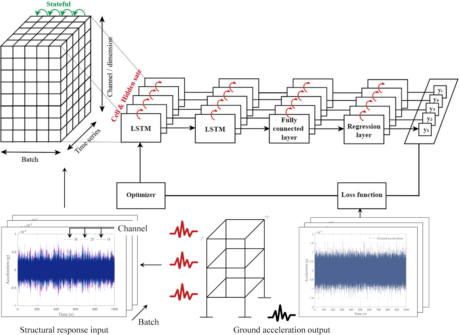
The EKF-LSTM approach developed in this study is a method of estimating the input load by constructing a network between the structural response and input load as an LSTM algorithm. Therefore, the input load becomes the output data in the LSTM algorithm and the structural response becomes the input data. Figure 1 shows a schematic diagram of the specific EKF-LSTM method developed in this study. In Fig. 1, the LSTM unit can be determined by the time series length or the number of time steps. In addition, in the LSTM unit, information about the time sequence of training data is transmitted through the cell state and hidden state. Regarding the learning process in Fig. 1, structural responses as long as the time series are input into the LSTM unit as input data. After passing through the learning layers of the LSTM layers, fully connected layer, and regression layer, the predicted output and output of the input load, which constitute the output data, are compared with a loss function, and the weight of the LSTM unit is updated using the optimizer. As learning by batch progresses, learning state information of time series data between batches is delivered by stateful. Therefore, the time series of the training data is learned dependently regardless of the batch. Further details on the LSTM algorithm can be found in the literature [60, 61]. Furthermore, the loss function used in this research as the mean square error is determined by Eq. (21).
(21)
In Eq. (21),
In addition, the adaptive moment estimation (Adam) optimizer applied for optimizing the weight value was proposed by [62]. The weight value update of the train network is determined by the following Eq. (22).
(22)
Figure 1.
Schematic of LSTM for the estimation process of input loads.
2.4EKF-LSTM
The general flowchart for EKF-LSTM is as shown in Fig. 2. To compose the LSTM network that can estimate the input load, the structural response and the input load, which is the ground acceleration, are acquired from the SI target structure. The network using the obtained structural response and input load as training data is trained through LSTM as shown in Fig. 1. Training proceeds only for the initially set max epoch. The initial state vector is established to use the EKF method for SI. The input load that was estimated through the LSTM network trained during the calculation of the predicted state space equation is used. This study is composed of a state vector that includes the modal responses, frequency, and damping ratio for estimating the modal parameters as shown in Eq. (19). In addition, as mentioned in Section 2.2, the sensor measurement data
Figure 2.
Flowchart for EKF-LSTM.
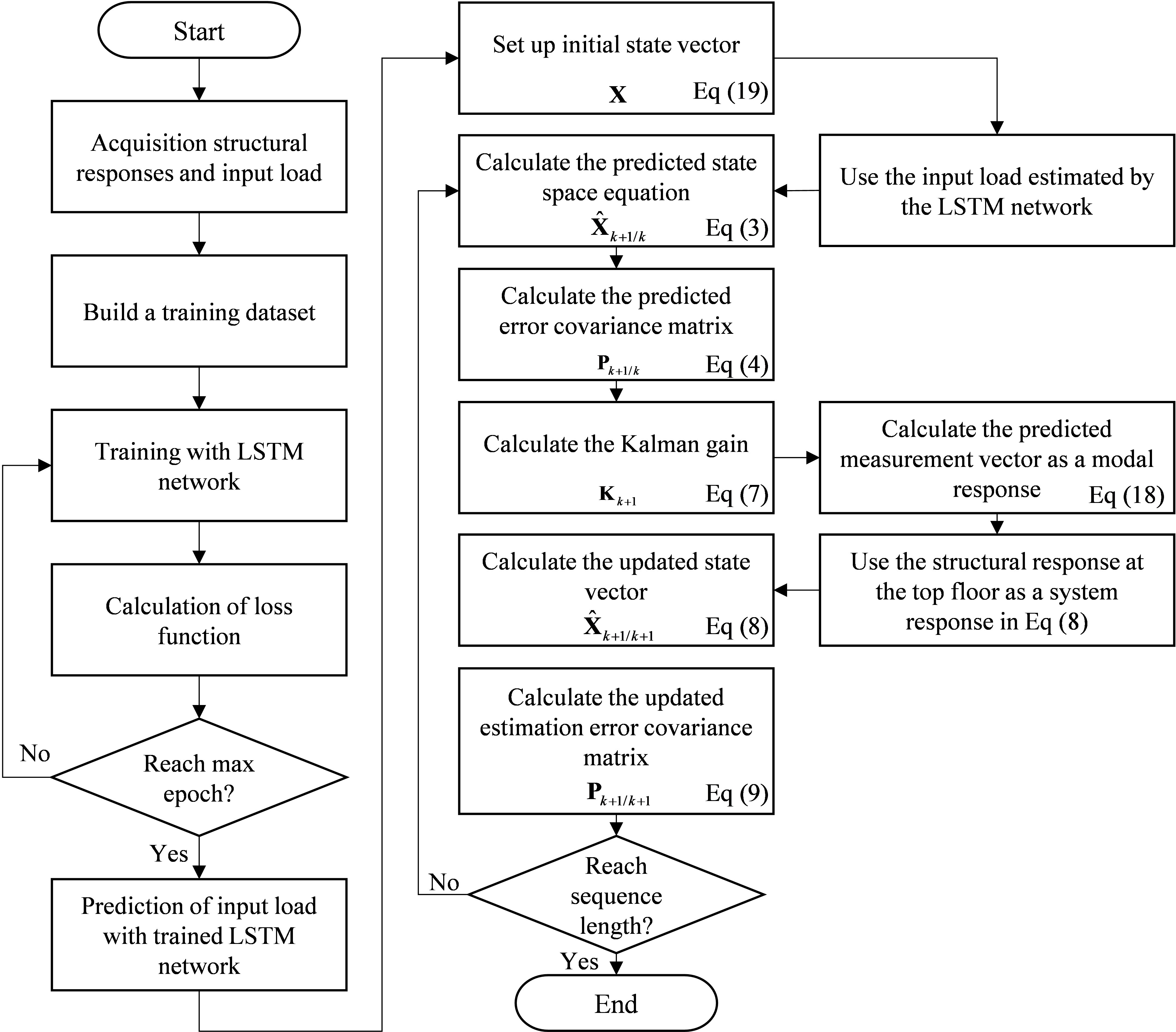
Figure 3.
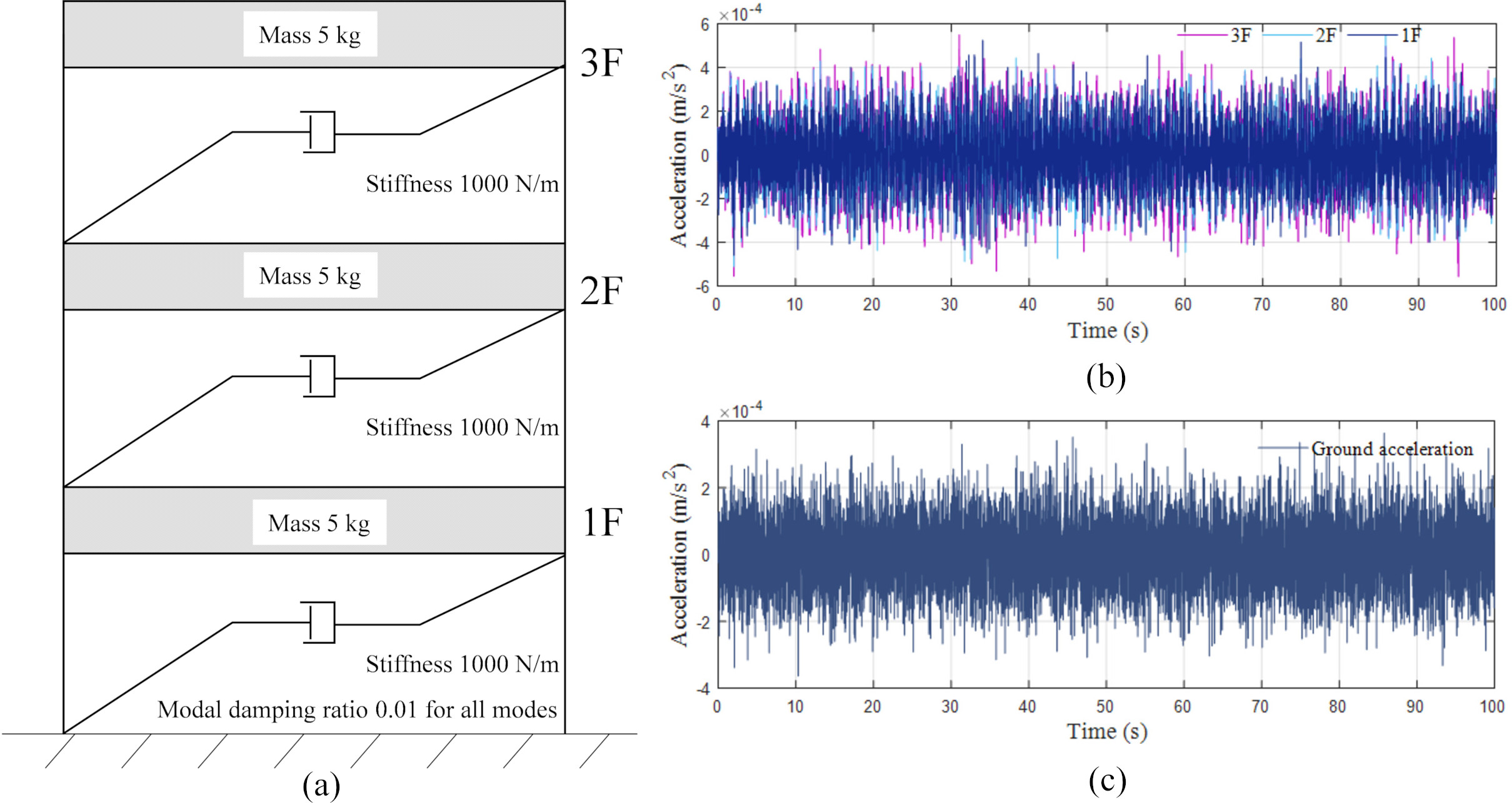
Training data obtained in numerical verification model: (a) System parameters of 3-DOF model; (b) Structural response used for the input; (c) Ground acceleration used for the output.
3.Numerical verification
3.13-DOF numerical model
To verify the proposed method, a dynamic system model with three 3-DOF was constructed and structural responses were obtained through Newmark numerical analysis. The specific system parameters for the model included a mass of 5 kg for each of the first, second, and third floors, with each floor having a stiffness of 1000 N/m. When the model was subjected to eigen value decomposition (EVD), the natural angular frequency was approximately 6.29 rad/s, 17.63 rad/s, and 25.48 rad/s for the first, second, and third modes, respectively, and the damping ratio for each mode was assumed to be 1%. The applied load was a white-noise input load. Furthermore, the sampling frequency is 100 Hz. Figure 3 shows the training data used as input and output data. To divide the training data shown in Fig. 3 into the input and output datasets, 200 pieces of data were generated for each dataset and used for LSTM learning. The learning rate was 0.001, minibatch size was 20, maximum epoch was 5,000, and maximum number of iterations was 50,000. The gradual decrease of the loss function in Fig. 4 indicates that the LSTM network was trained normally.
Figure 4.
Loss function of long short-term memory (LSTM).
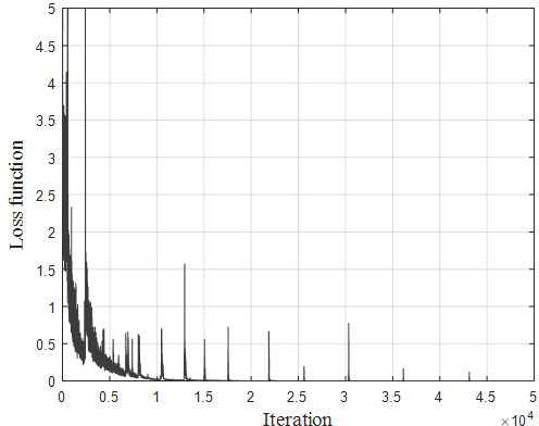
Figure 5.
Estimated ground acceleration from LSTM: (a) Comparison between the estimated and the exact ground accelerations, and (b) Scatter plot of predicted and exact results.
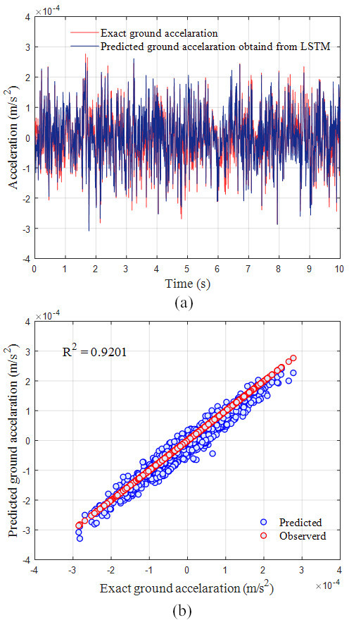
Figure 5a compares the estimated and exact ground acceleration results. As shown on the time axis of Fig. 3b, the training was conducted with a time series length of 100 s, but the LSTM algorithm showed results over 10 s. As such, the LSTM algorithm enabled estimation regardless of time. To compare the similarity between the exact ground acceleration and input load estimated by LSTM, the RMS results were compared. The RMS results can be used as a good index for representing the average for the signal that intersects the 0-axis. The root-mean-square (RMS) result for the exact ground acceleration was 9.8739e
Table 1
Modal parameter results identified as EKF-LSTM and EKF
| Methods | Mode | Natural angular frequency (rad/s) | Modal damping ratio | ||||||
|---|---|---|---|---|---|---|---|---|---|
| Exact | Identified without noise | SNR 20 dB | Error (%) | Exact | Identified without noise | SNR 20 dB | Error (%) | ||
| EKF-LSTM (EKF) | 1 | 6.29 | 6.29 (6.28) | 6.23 (6.27) | 0.00 | ||||
| (0.15) | 0.01 | 0.0101 (0.0103) | 0.0096 (0.0097) | 1.0 (3.0) | |||||
| 2 | 17.63 | 17.64 (17.59) | 18.15 (18.05) | 0.06 (0.22) | 0.01 | 0.0099 (0.0101) | 0.0095 (0.0096) | 1.0 (1.0) | |
| 3 | 25.48 | 25.60 (25.44) | 24.03 (24.52) | 0.47 (0.15) | 0.01 | 0.0098 (0.0103) | 0.0118 (0.0116) | 2.0 (3.0) | |
Figure 6.
Natural frequency estimation and relative error plots. (a) Natural frequency and (b) Modal damping ratio.
As it is necessary to set the initial values of the state variables of the initial state vector to execute EKF-based SI, the initial values for modal responses up to the third mode were set to zero, the natural angular frequencies and the modal damping ratios were set to
Figure 7.
System response estimation: (a) 1
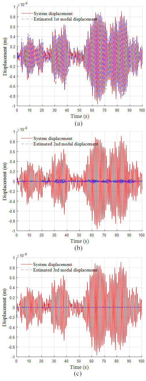
Table 1 presents the identification results using the EKF-LSTM and conventional EKF methods. To examine the impact of noise on the EKF-LSTM method, results for the case of the signal noise ratio (SNR) or the input and structural response being 20 dB was included. The LSTM network for estimating the input load when SNR
Furthermore, the EKF-LSTM method can estimate the modal response because it is composed of state variables, as indicated in Eq. (19). Figure 7 presents the modal displacement responses of the first through third modes estimated on the third floor. Figure 7a shows the first modal displacement response, which is already similar to the system displacement response with only the first mode. This indicates that the contribution of the first modal response to the system response was large. Because the sum of the first through third modal displacement responses represents the system displacement response, the RMS result of adding all the modal responses obtained from the EKF-LSTM method was estimated to be 3.3149e
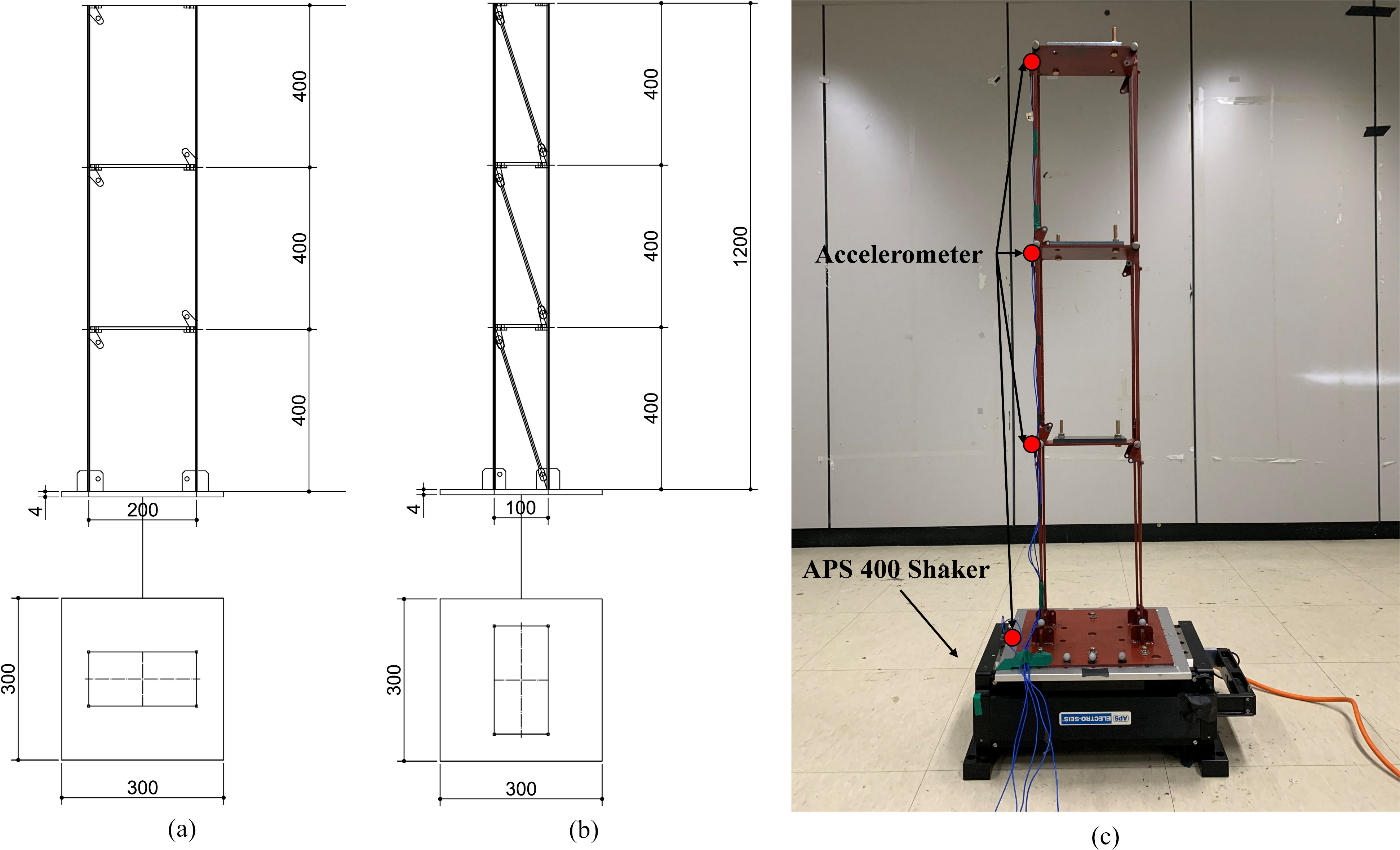
Figure 8.
Steel-frame structure model design: (a) Front view, (b) Side view, (c) Experiment model.
4.Experimental verification
4.1Experiment verification using steel-frame structure
In this section, the structural response was obtained by performing excitation experiments on the steel frame structure model, and the effectiveness of the EKF-LSTM method was verified using this response. The design information about the steel frame structure used in the study is provided in Fig. 8. The accelerometer used was a PCB333B50 sensor from PCB, which had a sensitivity of 1000 mV/g and a full-scale range of
The responses for approximately 235 s were used as the training data by selecting only the responses with white noise from the measurement data for the initial 300 s. Figure 9 shows the acquired training data.
The obtained response was subjected to a fast Fourier transform (FFT) to obtain the natural frequency and mode vector of the steel frame structure model. When the FFT was performed, the natural frequencies were obtained as 4.48 Hz, 14.08 Hz, and 20.09 Hz for the first, second, and third modes, corresponding to 28.148 rad/s, 88.467 rad/s, and 126.229 rad/s, respectively. Because the mode vector result corresponding to the natural frequency showed the first through third eigen shapes in Fig. 10b, the measurements seemed to have been performed accurately.
Figure 9.
Training data: (a) Acceleration for the input and (b) ground acceleration for the output.
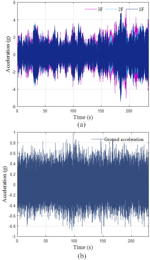
Figure 10.
Modal parameters of steel frame model.
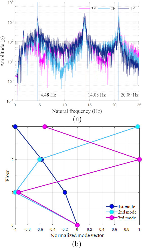
The modal assurance criterion (MAC) was calculated based on the acquired mode vector to apply the FDD method, and the modal damping ratio was identified using a spectral bell function of MAC 0.9 or higher. The modal damping ratios obtained through the FDD method were 0.0113, 0.0055, and 0.0033 for the first, second, and third modes, respectively. To use the training data in Fig. 9 for learning, the 60,000 data points for the total time series were divided into groups of 400 data points, yielding 150 training data sets. Among them, 30 data sets (20%) were used as test data. As for the hyperparameter settings for learning, the learning rate was set to 0.0001, batch size to 60, and maximum epoch to 200,000. Figure 11 shows the loss function of the trained LSTM network. As the learning progressed 400,000 times, the loss function curve gradually converged, suggesting that the learning had progressed normally.
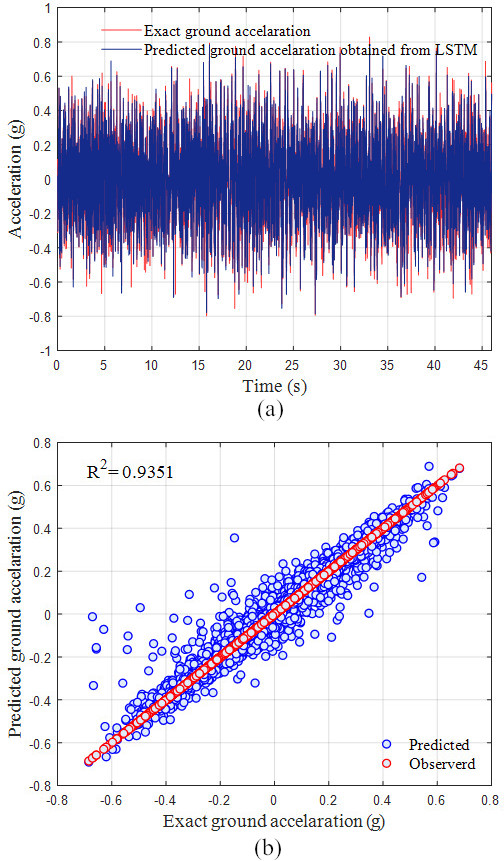
There were 30 test datasets in total, and considering that each dataset had 400 data points and the sampling frequency was 256 Hz, each dataset corresponded to approximately 1.56 s. Therefore, the test data had a time series length of approximately 46 s, and Fig. 12a shows the ground acceleration predicted by the LSTM network for 46 s. In the R-squared result representing the regression scale of the scatter plot in Fig. 12b, approximately 93% of the curve fitting is shown.
Figure 11.
Loss function plot as a function of the number of iterations.
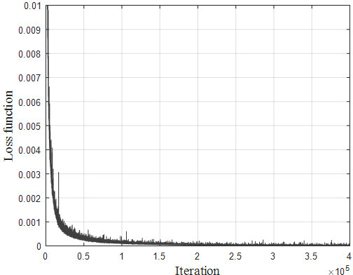
Figure 12.
Estimated ground acceleration based on LSTM: (a) Acceleration plot as a function of time, and (b) Scatter plot.
SI was performed using the predicted ground acceleration in Fig. 12 for the EKF. To execute the EKF, the initial modal responses up to the third mode were set to zero, the natural angular frequencies and the modal damping ratios were set to
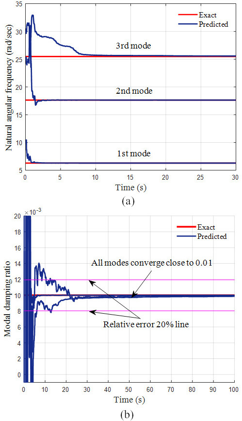
Figure 13.
Modal parameters of steel frame structure (a) Estimated natural frequencies, and (b) Modal damping ratio.
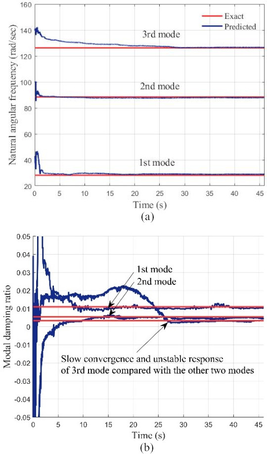
Table 2
Modal parameters identified from each method
| Mode | Natural angular frequency (rad/s) | Modal damping ratio | ||||
| EKF-LSTM | FDD | Error (%) | EKF-LSTM | FDD | Error (%) | |
| 1 | 28.360 | 28.148 | 0.75 | 0.0105 | 0.0113 | 7.1 |
| 2 | 88.710 | 88.467 | 0.2 | 0.0051 | 0.0055 | 7.2 |
| 3 | 126.882 | 126.229 | 0.5 | 0.0028 | 0.0033 | 15 |
Figure 14.
Estimated responses: (a) system and estimated acceleration responses, and corresponding responses for the (b) 1st, (c) 2nd, (d) 3rd modal accelerations
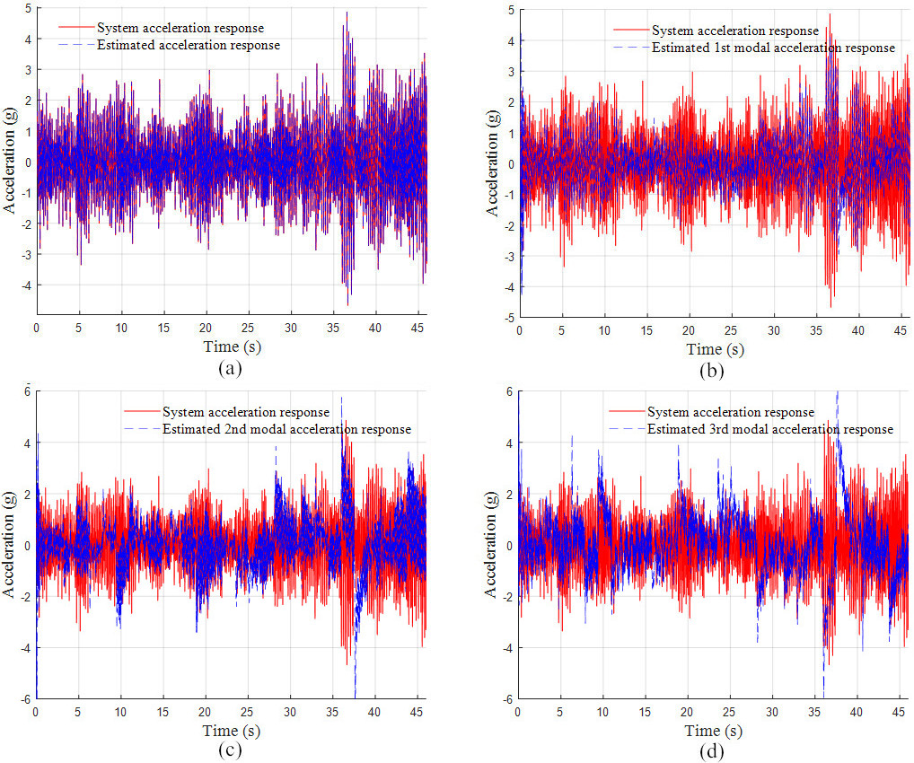
Figure 13 shows the modal parameters estimated by the EKF-LSTM method. As shown in Fig. 13a, the natural angular frequency was calculated to be 28.148 rad/s, 88.467 rad/s, and 126.229 rad/s for the first, second, and third modes, respectively. The predicted first natural angular frequency was 28.36 rad/s when the RMS was averaged after 10 s, showing a relative error of 0.75% from the results obtained by FFT. In addition, the predicted second natural angular frequency was 88.71 rad/s, indicating a relative error of approximately 0.2%. The predicted third natural angular frequency showed a slower convergence rate than the first and second modes, which may have been due to the low contribution of the third mode to the top floor response, as described in Section 2.2. The predicted third natural angular frequency was 126.882 rad/s from the RMS average at approximately 30 s, showing a relative error of approximately 0.5%. Figure 13b depicts the modal damping ratios, and the RMS results were identified as being 0.0105 and 0.0051 for the first and second modes, respectively, after approximately 10 s. These results indicated a difference of approximately 7% between the results identified by the FDD method and the maximum relative error. Considering the uncertainty of the modal damping ratio, the EKF-LSTM method seemed to show effective performance in the identification of the modal damping ratio. The third mode converged more slowly than the other modes, showing an unstable convergence curve, similar to the natural angular frequency result. This instability may have been due to the fact that the third mode had a low contribution to the system response. The RMS result from approximately 25 s after convergence was identified to be 0.0028.
Figure 14 shows the modal acceleration response estimated by the EKF. In the modal responses in Fig. 14b–d, the mode contribution to the system response changes with increasing mode order. In Fig. 14a, the response by adding all the first to third modal responses appears in a shape similar to the system acceleration response. The relative error between the average RMS result in Fig. 14a, which is the sum of the estimated modal responses, and the system response was calculated to be less than 1%. Table 2 summarizes the modal parameter estimation results by comparing the EKF-LSTM and FDD methods. To explain further, the modal response should show the shape of a sinusoidal wave, where the response scale becomes smaller for a higher mode. This tendency was not observed in Fig. 14b–d as the data were shuffled when composing the training data.
Figure 15.
Computational time for each method.
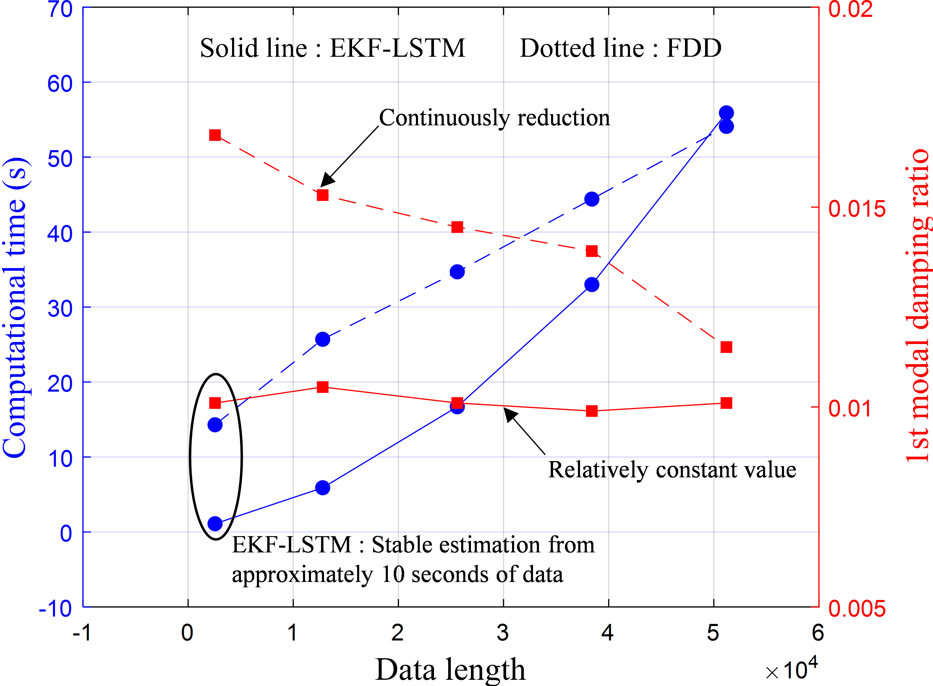
Figure 15 compares the computational time according to data length of the EKF-LSTM and FDD methods. In the application of EKF-LSTM, data was accumulated and the change in computational time had a parabolic form. The FDD method showed a linear pattern in the change in computational time, and this method could be considered to be more efficient. However, the results of the modal damping ratio of the FDD method shows a continuous decrease which approximated to about 0.01 from 200 s and above. Therefore, data for 200 s or above must be used for the application of the FDD method. In the application of the EKF-LSTM method, results of about 0.01 is obtained relatively constantly from about 10 s data. Thus, the computation of EKF-LSTM method was concluded to be more efficient. This method based on the EKF algorithm is able to estimate data real-time for each discrete time delta
To summarize the results obtained for the steel frame structure model using the EKF-LSTM method, the estimated natural angular frequency showed an error of less than 1%; the modal damping ratio, which has a relatively large error, shows an error within about 15%. Furthermore, the sum of the modal response showed an estimation result of less than 1% error compared with the displacement response. Among the results of the modal parameters, the modal damping ratio showed a rather large error of 15%, but it was still judged to be reliable considering the uncertainty of the modal damping ratio. Therefore, the effectiveness of the EKF-LSTM method proposed in this study is demonstrated in actual structural applications.
5.Conclusions
This research proposes the EKF-LSTM method that discerns the modal parameters with unknown input and without computational burden. This method was verified through the 3 DOF dynamic system model, and all modal parameters were distinguished with less than 2% maximum relative error. Further, less than 1% identification of natural angular frequency was shown in the validation through the steel frame structure model with 3 floors. For the modal damping ratio, a somewhat large difference of 15% was shown in the third mode. Only the top floor responses were used, which is why the contribution of the third mode was low and error had occurred. Considering the uncertainty of the modal damping ratio and that the difference was at the third decimal digit, the modal damping ratio results can be identified as a valid result. Additionally, the EKF-LSTM method shows that the modal damping ratio converges to a certain value from 10 seconds of data length from computational time according to the data length. Therefore, it was found to be advantageous in terms of the computational time in comparison to the conventional identification method.
The EKF-LSTM method only uses the top floor responses, and the estimation results lose accuracy as it approaches higher modes. If additional research could complement this drawback, the method will be practically applicable in actual buildings. The input load and structural response training data must be acquired before LSTM training for EKF-LSTM application in actual buildings. In actual buildings, input load and structural response may be impossible to obtain because ground loading is difficult. Therefore, to apply the EKF-LSTM method to real buildings, additional research must verify whether the input load and structural response obtained from the model updated finite element model that mocks the actual structural behavior can be used as training data. Further, research on the applicability of the input load as an alternative to the unobtainable ground acceleration is required by transforming the input load into the load of each floor.
Acknowledgments
This work was supported by a National Research Foundation of Korea (NRF) grant funded by the Korean Government (Ministry of Science, ICT & Future Planning, MSIP) (NRF-2021R1A2C33008989 and No. 2018R1A5A1025137).
References
[1] | Torzoni M, Rosafalco L, Manzoni A, Mariani S, Corigliano A. SHM under varying environmental conditions: an approach based on model order reduction and deep learning. Comput Struct. (2022) ; 266: : 106790. |
[2] | Luo J, Hong Y, Li C, Sun Y, Liu X, Yan Z. Frequency identification based on power spectral density transmissibility under unknown colored noise excitation. Comput Struct. (2022) ; 263: : 106741. |
[3] | Karami K, Fatehi P, Yazdani A. On-line system identification of structures using wavelet-Hilbert transform and sparse component analysis. Comput Civ Infrastruct Eng. (2020) ; 35: (8): 870-86. |
[4] | Park HS, Oh BK. Real-time structural health monitoring of a supertall building under construction based on visual modal identification strategy. Autom Constr. (2018) ; 85: : 273-89. |
[5] | Oh BK, Kim D, Park HS. Modal Response-Based Visual System Identification and Model Updating Methods for Building Structures. Comput Civ Infrastruct Eng. (2017) ; 32: (1): 34-56. |
[6] | Li Z, Park HS, Adeli H. New method for modal identification of super high-rise building structures using discretized synchrosqueezed wavelet and Hilbert transforms. Struct Des Tall Spec Build. (2017) ; 26: (3): 1-16. |
[7] | Perez-Ramirez CA, Amezquita-Sanchez JP, Adeli H, Valtierra-Rodriguez M, Camarena-Martinez D, Romero-Troncoso RJ. New methodology for modal parameters identification of smart civil structures using ambient vibrations and synchrosqueezed wavelet transform. Eng Appl Artif Intell. (2016) ; 48: : 1-12. doi: 10.1016/j.engappai.2015.10.005. |
[8] | Sirca GF, Adeli H. System identification in structural engineering. Vol. 19: , Scientia Iranica, (2012) . |
[9] | Adeli H, Jiang X. Dynamic fuzzy wavelet neural network model for structural system identification. J Struct Eng. (2006) ; 132: (1): 102-11. |
[10] | Jiang X, Adeli H. Dynamic wavelet neural network for nonlinear identification of highrise buildings. Comput Civ Infrastruct Eng. (2005) ; 20: (5). |
[11] | Zhou K, Li QS. Modal identification of high-rise buildings under earthquake excitations via an improved subspace methodology. J Build Eng. (2022) ; 52: : 104373. |
[12] | Huang Z, Xie M, Song H, Du Y. Modal analysis related safety-state evaluation of hidden frame supported glass curtain wall. J Build Eng. (2018) ; 20: : 671-8. |
[13] | Astroza R, Ebrahimian H, Conte JP, Restrepo JI, Hutchinson TC. Statistical analysis of the modal properties of a seismically-damaged five-story RC building identified using ambient vibration data. J Build Eng. (2022) ; 52: : 104411. |
[14] | Aumjaud P, Smith CW, Evans KE. A novel viscoelastic damping treatment for honeycomb sandwich structures. Compos Struct. (2015) ; 119: : 322-32. |
[15] | Xie X, Zheng H, Jonckheere S, Pluymers B, Desmet W. A parametric model order reduction technique for inverse viscoelastic material identification. Comput Struct. (2019) ; 212: : 188-98. |
[16] | Zhang H, Ding X, Wang Q, Ni W, Li H. Topology optimization of composite material with high broadband damping. Comput Struct. (2020) ; 239: : 106331. |
[17] | Kasinos S, Palmeri A, Lombardo M, Adhikari S. A reduced modal subspace approach for damped stochastic dynamic systems. Comput Struct. (2021) ; 257: : 106651. |
[18] | Brincker R, Ventura CE, Andersen P. Damping estimation by frequency domain decomposition. In: Proceedings of the International Modal Analysis Conference – IMAC. (2001) . pp. 5-8. Available from: https://svibs.testlakrids.dk/wp-content/uploads/2019/12/2001_4.pdf. |
[19] | Peeters B, De Roeck G. Reference-based stochastic subspace identification for output-only modal analysis. Mech Syst Signal Process. (1999) ; 13: (6): 855-78. |
[20] | Peeters B, De Roeck G. Stochastic System Identification for Operational Modal Analysis: A Review. J Dyn Syst Meas Control. (2001) Dec 1; 123: (4): 659-67. |
[21] | Xu K, Mita A. Maximum drift estimation based on only one accelerometer for damaged shear structures with unknown parameters. J Build Eng. (2022) ; 46: : 103372. |
[22] | Chen Y, Castiglione J, Astroza R, Li Y. Parameter estimation of resistor-capacitor models for building thermal dynamics using the unscented Kalman filter. J Build Eng. (2021) ; 34: : 101639. |
[23] | Huang K, Yuen KV, Wang L, Jiang T, Dai L. Sensor fault detection, localization, and reconstruction for online structural identification. Struct Control Heal Monit. (2022) (June 2021); 1-22. |
[24] | Hu Z, Gallacher B. Extended Kalman filtering based parameter estimation and drift compensation for a MEMS rate integrating gyroscope. Sensors Actuators A Phys, (2016) ; 250: . |
[25] | Li H, Mao CX, Ou JP. Identification of Hysteretic Dynamic Systems by Using Hybrid Extended Kalman Filter and Wavelet Multiresolution Analysis with Limited Observation. J Eng Mech. (2013) ; 139: (5). |
[26] | Liu JL, Yu AH, Chang CM, Ren WX, Zhang J. A new physical parameter identification method for shear frame structures under limited inputs and outputs. Adv Struct Eng. (2021) Mar 1; 24: (4): 667-79. |
[27] | Lei Y, Qiu H, Zhang F. Identification of structural element mass and stiffness changes using partial acceleration responses of chain-like systems under ambient excitations. J Sound Vib. (2020) ; 488: . |
[28] | Hoshiya M, Saito E. Structural identification by extended Kalman filter. J Eng Mech. (1984) ; 110: (12): 1757-70. |
[29] | Zhi L, Li QS, Fang M. Identification of Wind Loads and Estimation of Structural Responses of Super-Tall Buildings by an Inverse Method. Comput Civ Infrastruct Eng. (2016) ; 31: (12): 966-82. |
[30] | Xiong R, He H, Sun F, Zhao K. Evaluation on State of Charge estimation of batteries with adaptive extended kalman filter by experiment approach. IEEE Trans Veh Technol. (2013) ; 62: (1): 108-17. |
[31] | Jeen-Shang L, Yigong Z. Nonlinear structural identification using extended kalman filter. Comput Struct. (1994) ; 52: (4): 757-64. |
[32] | Song M, Astroza R, Ebrahimian H, Moaveni B, Papadimitriou C. Adaptive Kalman filters for nonlinear finite element model updating. Mech Syst Signal Process. (2020) ; 143: : 106837. |
[33] | Al-Hussein A, Haldar A. Nonlinear system identification from noisy measurements. Int J Struct Eng. (2018) ; 9: (2): 154-73. |
[34] | Lei Y, Liu C, Liu LJ. Identification of multistory shear buildings under unknown earthquake excitation using partial output measurements: Numerical and experimental studies. Struct Control Heal Monit. (2014) ; 21: (5): 774-83. |
[35] | Meiliang W, Smyth AW. Application of the unscented Kalman filter for real-time nonlinear structural system identification. Struct Control Heal Monit. (2007) ; 14: (7): 971-90. |
[36] | Roveda L, Piga D. Sensorless environment stiffness and interaction force estimation for impedance control tuning in robotized interaction tasks. Auton Robots. (2021) ; 45: (3). |
[37] | Zhang C, Gao YW, Huang JP, Huang JZ, Song GQ. Damage identification in bridge structures subject to moving vehicle based on extended Kalman filter with l1-norm regularization. Inverse Probl Sci Eng. (2020) ; 28: (2). |
[38] | Huang Y, Zhang Y, Wu Z, Li N, Chambers J. A Novel Adaptive Kalman Filter with Inaccurate Process and Measurement Noise Covariance Matrices. IEEE Trans Automat Contr. (2018) ; 63: (2): 594-601. |
[39] | Wang H, Deng Z, Feng B, Ma H, Xia Y. An adaptive Kalman filter estimating process noise covariance. Neurocomputing. (2017) ; 223: : 12-7. |
[40] | Bisht SS, Singh MP. An adaptive unscented Kalman filter for tracking sudden stiffness changes. Mech Syst Signal Process. (2014) ; 49: (1-2): 181-95. |
[41] | Yun DY, Hong T, Lee DE, Park HS. Structural Damage Identification with a Tuning-free Hybrid Extended Kalman Filter. Struct Eng Int. (2021) ; 31: (3): 391-405. |
[42] | Kim D, Oh BK, Park HS, Shim HB, Kim J. Modal Identification for High-Rise Building Structures Using Orthogonality of Filtered Response Vectors. Comput Civ Infrastruct Eng. (2017) ; 32: (12): 1064-84. |
[43] | Yang JN, Pan S, Huang H. An adaptive extended Kalman filter for structural damage identifications II: Unknown inputs. Struct Control Heal Monit. (2007) ; 14: (3): 497-521. |
[44] | García-Palencia AJ, Santini-Bell E. A two-step model updating algorithm for parameter identification of linear elastic damped structures. Comput Civ Infrastruct Eng. (2013) ; 28: (7): 509-21. |
[45] | Pan S, Xiao D, Xing S, Law SS, Du P, Li Y. A general extended Kalman filter for simultaneous estimation of system and unknown inputs. Eng Struct. (2016) ; 109: : 85-98. |
[46] | Yun DY, Kim D, Kim M, Bae SG, Choi JW, Shim HB, Hong T, Lee DE, Park HS. Field measurements for identification of modal parameters for high-rise buildings under construction or in use. Autom Constr. (2021) ; 121: : 103446. |
[47] | Yang JN, Lin S, Huang H, Zhou L. An adaptive extended Kalman filter for structural damage identification. Struct Control Heal Monit. (2006) ; 13: (4): 849-67. |
[48] | Al-Hussein A, Haldar A. Unscented Kalman filter with unknown input and weighted global iteration for health assessment of large structural systems. Struct Control Heal Monit. (2016) ; 23: (1): 156-75. |
[49] | Kim H, Sim SH. Automated peak picking using region-based convolutional neural network for operational modal analysis. Struct Control Heal Monit. (2019) ; 26: (11): e2436. |
[50] | Liu D, Tang Z, Bao Y, Li H. Machine-learning-based methods for output-only structural modal identification. Struct Control Heal Monit. (2021) ; 28: (12): e2843. |
[51] | Impraimakis M, Smyth AW. Input-parameter-state estimation of limited information wind-excited systems using a sequential Kalman filter. Struct Control Heal Monit. (2022) ; 29: (4): e2919. |
[52] | Xu Y, Lu X, Cetiner B, Taciroglu E. Real-time regional seismic damage assessment framework based on long short-term memory neural network. Comput Civ Infrastruct Eng. (2021) ; 36: (4). |
[53] | Qarib H, Adeli H. A new adaptive algorithm for automated feature extraction in exponentially damped signals for health monitoring of smart structures. Smart Mater Struct. (2015) ; 24: (12). |
[54] | Amezquita-Sanchez JP, Adeli H. A new music-empirical wavelet transform methodology for time-frequency analysis of noisy nonlinear and non-stationary signals. Digit Signal Process A Rev J. (2015) ; 45: . |
[55] | Amezquita-Sanchez JP, Park HS, Adeli H. A novel methodology for modal parameters identification of large smart structures using MUSIC, empirical wavelet transform, and Hilbert transform. Eng Struct. (2017) ; 147: . |
[56] | Perez-Ramirez CA, Amezquita-Sanchez JP, Valtierra-Rodriguez M, Adeli H, Dominguez-Gonzalez A, Romero-Troncoso RJ. Recurrent neural network model with Bayesian training and mutual information for response prediction of large buildings. Eng Struct. (2019) ; 178: . |
[57] | Oh BK, Kim KJ, Kim Y, Park HS, Adeli H. Evolutionary learning based sustainable strain sensing model for structural health monitoring of high-rise buildings. Appl Soft Comput J. (2017) ; 58: . |
[58] | Eftekhar Azam S, Chatzi E, Papadimitriou C. A dual Kalman filter approach for state estimation via output-only acceleration measurements. Mech Syst Signal Process. (2015) ; 60: : 866-86. |
[59] | Kalman RE, Bucy RS. New results in linear filtering and prediction theory. J Fluids Eng Trans ASME. (1961) ; 83: (1). |
[60] | Hochreiter S. The vanishing gradient problem during learning recurrent neural nets and problem solutions. Int J Uncertainty, Fuzziness Knowlege-Based Syst. (1998) ; 6: (2): 107-16. |
[61] | Hochreiter S, Schmidhuber J. Long Short Term Memory. Neural Computation. (1997) ; 9: (8): 1735-80. |
[62] | Kingma DP, Ba J. Adam: A Method for Stochastic Optimization. BT – 3rd International Conference on Learning Representations, ICLR 2015, San Diego, CA, USA, May 7-9, 2015, Conference Track Proceedings. International Conference on Learning Representations (ICLR). (2015) . |
[63] | Ruder S. An overview of gradient descent optimization algorithms. (2016) ; 1-14. Available from: http://arxiv.org/abs/1609.04747. |


