
Artificial intelligence and machine learning: Practical aspects of overfitting and regularization
Abstract
Neural networks can be used to fit complex models to high dimensional data. High dimensionality often obscures the fact that the model overfits the data and it often arises in the publication industry because we are usually interested in a large number of concepts; for example, a moderate thesaurus will contain thousands of concepts. In addition, the discovery of ideas, sentiments, tendencies, and context requires that our modelling algorithms be aware of many different features such as the words themselves, length of sentences (and paragraphs), word frequency counts, phrases, punctuation, number of references, and links. Overfitting can be counterbalanced by Regularization, but the latter can also cause problems. This paper attempts to clarify the concepts of “overfitting” and “regularization” using two-dimensional graphs that demonstrate over fitting and how regularization can force a smoother fit to noisy data.
1.Introduction
Why should publishers and other data/information providers be interested in Artificial Intelligence (AI) and Machine Learning (ML)? Any classification problem for which a good source of classified examples exists (data for which they already know the correct classification; e.g. bibliographic data, citations, keywords, datasets, etc.) is a good candidate for AI. Historically, character recognition (OCR) was a difficult problem for publishers attempting to digitize their print collections. But today they benefit from enormous improvement in the performance of OCR because, at least in part, a very large collection of already-classified examples now exists. Similarly, automatic translation between languages (such as English, French, German, Latin, Spanish, etc.) has made tremendous advances because enormous collections of already-translated documents can be accessed and used to train the classifying algorithm. Other contexts that seem to recommend themselves to publishers for the use of Machine Learning and Artificial Intelligence are concept identification in texts, entity (people, places, things) extraction, assigning reviewers to submitted documents, sentiment analysis, quality evaluation, and priority assignment of submitted manuscripts. In each of these situations, the application of AI and ML will require the development of a set of algorithms, entitled “neural networks”. These networks are modeled loosely after the human brain and are designed to recognize patterns via the AI/ML “models” that must be built to analyze the content/data in question. The models that are developed must smoothly “fit” the sample data that is being used to build them in order to generate correct classifications for the broader corpus of data. Therefore the sample data required must be as “close” to a “typical” example of the data being classified like that example to which it is “near”- and this is the fundamental idea behind classification and model fitting. The goal of this paper is to highlight the key challenges to building effective and efficient models.
2.Understanding the challenges with machine learning and artificial intelligence
The data found in the publishing industry is often high dimensional in nature. High dimensionality arises because publishers are usually interested in a large number of concepts; for example, a moderate thesaurus will contain thousands of concepts. Useful text will have a large number of words. Therefore, the utilization of AI and ML for the discovery of ideas, sentiments, tendencies, and context requires that the algorithms be aware of many different features such as the words themselves, the length of sentences (and paragraphs), word frequency counts, phrases, punctuation, number of references, and links.
The key points to keep in mind with regards to understanding the challenges with Machine Learning and Artificial Intelligence are as follows:
1. High dimension obscures data trends: In two dimensions we can graph some data on a piece of two-dimensional paper and see correlations. Projecting three-dimensional data onto a two-dimensional piece of paper can cause correlations to disappear. Suppose that z = x + y. And you look at the data in the x, z plane. You can see points scattered randomly in the x, z plane with no obvious correlation. And we are often interested in using hundreds or thousands of dimensions. Each added dimension can obscure relationships much like z = x + y mixes the changes in value of x and y.
2. Large numbers of adjustable parameters provide for overfitting models: One of the first mistakes a student makes when they learn to use polynomials to fit data, is to increase the order of the polynomial to “improve the fit” while completely ignoring the fact that the measured data is guaranteed to contain random errors that will mislead the analysis. My example of a straight line explores this mistake and shows that this leads to models that fit the noise and wildly disagree with reality. The number of adjustable parameters should always be smaller than the number of measurements. A polynomial of order n has n + 1 adjustable parameters.
3. Projecting into two dimensions often cannot convey the complexity of the situation as you can see by looking at the z = x + y model: If the relationship was that z = x, we could see it easily in a plot of z versus x. But if z = x + y, and we project into the two dimensions of z and x we will see figures that depend on the fortuitous and unknown values of y. That is, we could see absolutely no relationship at all! In real life we would probably get some clues from the two-dimensional graph. But we could also be wildly misled by fortuitous values of the third variable.
4. Principle Component Analysis is a method from linear algebra for detecting linear correlations in high dimensional data: PCA will automatically detect correlations of the form z = x + y. Of course, the correlations that we are searching for will often be more complex than this simple linear case. For example, PCA will not detect a correlation in the shape of a circle.
In order to present data that you can actually see, some simple, two-dimensional examples where the problems are not overwhelmed by dimensionality are included below. First, however, let’s explore these challenges further.
3.Large numbers of adjustable parameters provide for overfitting models
One of the ubiquitous problems encountered in machine learning is overfitting. Overfitting occurs when a proposed predictive model is so complex that it fits the noise, or the non-reproducible part, of the data. There are two critical problems that lead to overfitting. They are data uncertainty and model uncertainty. These two problems interact with one another. That is, you cannot deal with one without the other. Overfitting is described in more detail below.
3.1.Data uncertainty
Data uncertainty occurs because real data has measurement errors. For example, if you measure your waist circumference with a tape measure with 0.01 inch fiduciary marks, you will get a different value every time you make the measurement.
Data uncertainly also occurs because quantum mechanics guarantees it. There are no point masses in the real world. Everything becomes “fuzzy” if you look at it closely. The closer you look, the fuzzier it gets. If you look closely enough everything gets completely fuzzy. If you look very closely at an electron, it becomes a wave.
3.2.Model uncertainty
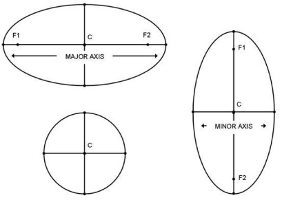
No model is perfect. All models are approximations to reality. One of our common models is that the earth as rotating about the sun in an elliptical orbit. But that orbit is perturbed by the gravitational influence of Jupiter, Saturn, the moon, and everything else in the, including you and me. It is only approximately elliptical. The model becomes approximate if we look at it closely.
Another common model is that things have locations. For example, your house is on a lot that has corners with absolute, known locations. Metal stakes are driven into the ground to mark the corners. Yet, we know that the earth’s surface is deforming. The continents are drifting along with your house. These two models predict different facets of reality. We normally ignore continental drift relative to real estate transactions. When do we need to account for the continental drift of your house?
3.3.Balancing errors
Another pitfall in AI and ML is balancing errors. Measurement errors (data uncertainty) and model errors (model uncertainty) must be consistent. For example, if we learned to live for millions of years, we might need to account for continental drift deforming ground around our home and the location of our home in our real estate transactions. But for short time scales, we can ignore the model errors associated with neglecting the effects of continental drift. And we need only to worry about the location of the corners of the property that we assume are constant and immovable.
Using the minimization of the square error methodology, we adjust the model coefficients to minimize the summed square errors between the predicted values and the observed values as is demonstrated by the following example associated with Carl Fredrick Gauss recovering the orbit of Ceres from noisy data.
Example: Lost Planets and Regularization
 Giuseppe Piazzi, an Italian astronomer (among other disciplines), discovered the dwarf planet Ceres on January 1, 1801. He made twenty-one measurements over forty days spanning nine degrees across the sky. When he tried to view it again in February, however, it did not appear where he expected. Imagine his relief when Ceres was discovered again on December 31st of that same year in a location predicted by Carl Friedrich Gauss, a German mathematician (also among other disciplines).
Giuseppe Piazzi – https://it.wikipedia.org/wiki/Giuseppe_Piazzi
Piazzi and others thought that the orbit of Ceres was circular. They used a circular orbit as the model for the orbit of Ceres and were unable to locate it. Gauss used an elliptic orbit as a model - found Ceres. Piazzi and his associates were using the wrong mode - in addition to not employing the least squares error methodology.
Carl Friedrich Gauss made two major changes to the model fitting process relative to his predecessors. One important change is that he adjusted the orbit parameters to minimize the sum of the squared error (employed the least squares methodology) between the observed measurements and the predictions of the elliptic orbit model. This allowed him to use more of the observations to get an improved estimate of the orbit parameters. The second major change is that he forced the model to be an elliptic orbit. This was his “regularization” assumption, eliminating wilder variations that are available with straight line and circular motion models. In this sense, he forced his model to be “more realistic” or “regular”. However, the orbit of Ceres is not exactly elliptical. Ceres is moving under the gravitational influence of the sun and other planets (especially Jupiter) as well. Ceres would move in a precise elliptic orbit if it was moving under the gravitational influence of ONLY the sun. Because of the gravitational effect of the other planets, it actually wobbles about, approximating an elliptic orbit, but distorted because it is under the influence of the gravity of other objects (like Jupiter and the Milky Way). It does not follow an exactly elliptic orbit. At this point, an elliptic orbit is simply a better model than either a straight line or a circle. How would you regularize to allow for slight variations from an elliptic orbit?
3.4.Regularization
In basic terms, regularization is adding constraints or generalizing the model in order to improve its predictions (by making it more “regular” or “smoother” or “consistent with reality”). Regularization is essentially an iterative process. We start with data and build a model. We adjust the model parameters to minimize the square error between the model predictions and observations. Then we use the model to make predictions. When the predictions disagree with the observations by more than the statistical uncertainty in the measurements, we adjust the model.
4.Fitting and noisy data
4.1.Getting to the perfect fit
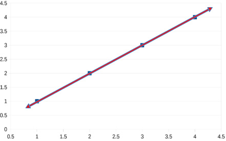
Consider some data that has no uncertainty (noise). On a graph with an XY axis, a straight line can be fit to the four points that have the values (1,1), (2,2), (3,3), and (4,4). Since a straight line is completely determined by a pair of points on the line, we can draw one straight line that goes through all four of these points as shown in Fig. 1.
Fig. 1.
Data that has no uncertainty (noise).
More advanced mathematics tells us that we can also fit an infinite number of 4th degree polynomials to these four points. Each of the infinite number of 4th degree polynomials will exactly match the four specified points if we use infinite precision arithmetic as noted in Fig. 2.
Fig. 2.
Infinite number of 4th degree polynomials.
The idea behind regularization is to penalize models that have this wild property while at the same time allowing physically reasonable variations in the model. The penalties that we can impose are only limited by our imagination and creativity. For example, we might arbitrarily assume that a straight line fits our data, and this might be a good model for a spring within its elastic range. It is a terrible model for the motion of a planet in its orbit if you want to predict its motion for a significant portion of an orbital period.
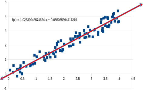
However, once we allow that data is uncertain or noisy, we must allow for the fact that a perfect fit is no longer possible nor desirable. That is, a perfect fit of a model to noisy data indicates that the model is fitting the noise. Each new data point will require a large increase in the complexity of the model because we are fitting a single-valued function to data that can have many values for the same value of the independent parameter.
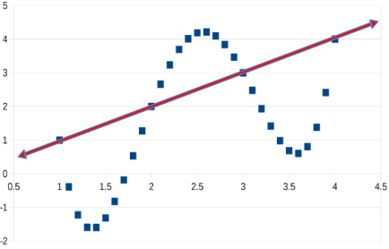
Fig. 3.
Noisy data fit by a straight line. We have “regularized” our fit by forcing the model to be a straight line with only 2 parameters.
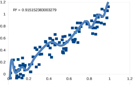
Ultimately, all that we can do is to predict the probability distribution of the results of measurements. Noise means that repeated measurements of the same thing will not produce the same values. We want to reduce the effect of noise on the model because we want to have confidence, not necessarily certainty, in the predictions of our model. Instead of reducing the effect of the noise, overfitting forces our models to become so complex that the model only fits the data at the measured points and varies wildly from those values everywhere else - see Fig. 4.
Fig. 4.
20th degree polynomial with 100 pts fitting the noise.
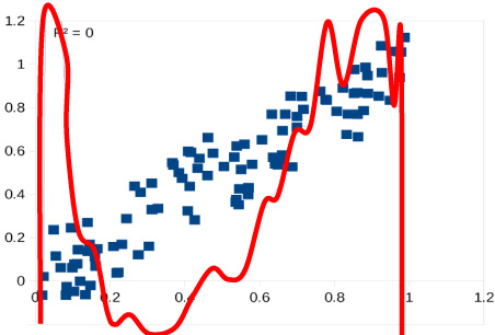
As the fit becomes more complex, predictability is reduced. In attempting to fix the model, we actually break it. This is what we are doing when we overfit our data and fit the random variations in our data with a complex model. Random variations force the model to make wild predictions (see Fig. 5).
Fig. 5.
60 degree polynomial numerical precision exceeded.
Consider a situation where we wish to measure something and we repeat the measurement. Each time we repeat the measurement we get a different value, yet we feel that the value did not change. Our normal model for this situation is simply that we made small errors in our measurement. Let us now think about a series of such measurements. For example, we might think about measuring the extension of a spring when the spring has different weights attached to it. We can repeat the measurement of the spring extension for each weight many times. Each measurement will produce a slightly different extension if we measure precisely enough. Does this mean that we should fit a vertical line to the data for each weight? This would not be a reasonable model.
4.2.Detecting overfitting
There is a simple test to see if you are overfitting. First, split the training data into two pieces. Use one to train the model and the second to test the quality of the “fit”. Your data will have uncertainty. When the uncertainty in your predictions becomes less than the uncertainty in your data, you may be overfitting.
There is a tradeoff between model error and measurement error. Reality is always more complex than your model and your data is always uncertain (noisy).
Minimizing the summed square errors between the model and the measurements gives the “best” estimate for the model parameters if the noise is “Normal”.
When we have an imperfect model and erroneous data, we need to balance the cost associated with the imperfect model with the cost of the erroneous data.
Overfitting is a constant challenge with any machine learning task. Because of the black box nature of most machine learning, and the fact that an overly complex model will often fit the same data “better”, we must constantly be on guard against overfitting. We need to balance the errors associated with measurements with errors associated with overfitting.
5.An example of overfitting
Consider a publishing firm that has five million articles in its corpus and wants to develop author profiles for peer review.
Machine Learning is applied to develop author profiles. Overfitting leads the AI to assign extremely granular concepts to authors. In this example, an author is an expert in the quantum entanglement discipline of physics. This extremely granular topic leads the machine to NOT suggest this author for peer review because they are not an expert in the broader topic of “Physics”.
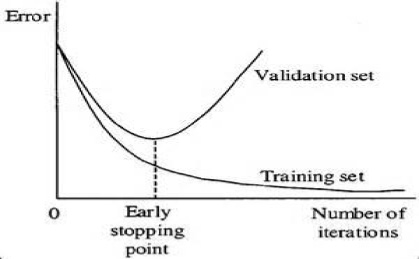
Stopping the training when performance on the validation data set decreases can reduce the impact of overfitting. Using a simpler model such as reducing the number of layers or nodes in the neural network can avoid overfitting. At the same time, an overly simple model may not fit a complex situation. Allowing the model to view broader level concepts like “physics” instead of just “quantum entanglement” can improve its performance.
6.Conclusion
A neural network (the set of AL/ML algorithms used for analysis) is basically a “feeling” machine. It senses correlations and generates feelings. The model underlying the network provides a framework for using the correlations to make predictions and classifications. Therefore, it is important to use models constrained to be physically reasonable and predict observations within their statistical uncertainty.
About the Author
Daniel Vasicek is a data scientist and engineer with experience indexing text at Access Innovations, laser communication with SAIC, petroleum prospecting with British Petroleum, and the Apollo Mission to the Moon with NASA. Contact information: Tel.: +1 (505) 265 3591. Email: Daniel_Vasicek@AccessInn.com.

