
A Novel Entropy Measure with its Application to the COPRAS Method in Complex Spherical Fuzzy Environment
Abstract
A complex spherical fuzzy set (CSFS) is a generalization of the spherical fuzzy set (SFS) to express the two-dimensional ambiguous information in which the range of positive, neutral and negative degrees occurs in the complex plane with the unit disk. Considering the vital importance of the concept of CSFSs which is gaining massive attention in the research area of two-dimensional uncertain information, we aim to establish a novel methodology for multi-criteria group decision-making (MCGDM). This methodology allows us to calculate both the weights of the decision-makers (DMs) and the weights of the criteria objectively. For this goal, we first introduce a new entropy measure function that measures the fuzziness degree associated with a CSFS to compute the unknown criteria weights in this methodology. Then, we present an innovative Complex Proportional Assessment (COPRAS) method based on the proposed entropy measure in the complex spherical fuzzy environment. Besides, we solve a strategic supplier selection problem which is very important to maximize the efficiency of the trading companies. Finally, we present some comparative analyses with some existing methods in different set theories, including the entropy measures, to show the feasibility and usefulness of the proposed method in the decision-making process.
1Introduction
In our world which is becoming a more global marketplace, the global environment is forcing companies to take almost everything into consideration at the same time, remain competitive and respond to rapidly changing markets. In this aspect, supply chain management and strategic sourcing have been one of the fastest-growing and most important areas of management in companies. Since technological complexity has affected the logistics and supply chains directly, the supply chain management has to adapt to these complex and dynamic factors. So, in this trading world, the search for new and strategic suppliers is a continuous priority for companies in order to upgrade the variety and typology of their product range. Hence, supplier selection represents one of the most important functions to be performed by the purchasing department that determines the long-term viability of a company. Strategic supplier selection is a multi-criteria problem that includes both qualitative and quantitative criteria. In order to select the best suppliers, it is necessary to make a tradeoff between tangible and intangible criteria, some of which may conflict. In this case, we are required to handle a decision-making problem.
Decision-making is the process of identifying different and possible alternatives that can solve a problem and choosing the one that will best meet the expectations among these alternatives. Since complexity prolongs the decision-making process, as it requires the evaluation of many alternatives according to many criteria in the process, many studies and decision-making methods have been developed in the literature to work with complex data and make an appropriate choice (Chen, 1988; Maji et al., 2001). Multi-criteria decision-making (MCDM) is one of the decision-making methods based on an expert’s opinion. If more than one expert is attending, this method is called MCGDM. In literature, there are many techniques that have been developed to solve MCDM and MCGDM problems such as the Analytic Hierarchy Process (AHP) (Saaty, 1980), Technique for Order Performance by Similarity to Ideal Solution (TOPSIS) (Hwang and Yoon, 1981), COPRAS (Zavadskas et al., 1994), VIsekriterijumsko optimizacija Kompromisno Rangiranje (VIKOR) (Opricovic, 1998), Multi-Objective Optimization by Ratio Analysis (MOORA) (Brauers and Zavadskas, 2006) and so on.
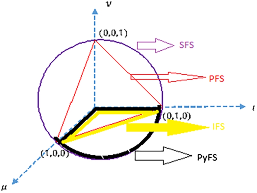
Fuzzy set (FS) theory (Zadeh, 1965) is an effective tool for solving decision-making problems in this increasingly complex world, as FS is a way of thinking used to describe the imprecise. However, since the evaluation is only made on the degree of membership in FS theory, this is also insufficient to solve complex problems. For this reason, many generalizations of FS theory have been made in the literature. The intuitionistic fuzzy set (IFS) (Atanassov, 2003) which is one of these generalizations, refers to a set whose sum of positive-membership degree and negative-membership degree is less than or equal to 1. After, the IFS theory was extended to Pythagorean fuzzy set (PyFS) (Yager, 2013) theory by considering the sum of the squares of its positive-membership degree and negative-membership degree is less than or equal to 1. The other extension of IFS is Picture Fuzzy Set (PFS) (Cuong, 2013) which has positive-membership, neutral-membership and negative-membership degrees and the sum of these degrees is less than or equal to 1. PFS is able to deal with problems that have more answers. Then the theory of SFS has been developed by Mahmood et al. (2018) to encounter situations that PFS cannot meet. In the SFS, the sum of the squares of positive-membership, neutral-membership and negative-membership degrees is less than or equal to 1. Many authors have studied on these sets (Aydoğdu and Gül, 2020; Güner and Aygün, 2020, 2022). Geometric representations of the theories IFS, PyFS, PFS and SFS are shown in Fig. 1. The mentioned set theories are highly proficient and skilled to carry ambiguous information but their capabilities are limited to handle one-dimensional data. Many MCDM problems comprise two-dimensional data but the existing MCDM strategies are incompetent to handle the two-dimensional information. To handle such phenomena, complex generalizations of FSs mentioned above have been studied by Ramot et al. (2002, 2003), Alkouri and Salleh (2013), Ullah et al. (2020), Akram et al. (2021c) and these sets have been applied to many decision-making problems. Azam et al. (2022) gave an example of evaluating the enterprise’s information security management issue in a particular organization on complex intuitionistic fuzzy sets (CIFSs). Akram et al. (2020) made an example of selecting the best capable ERP systems as candidates after collecting information about ERP vendors and systems from all aspects of the complex picture fuzzy set (CPFS) environment. Recently, Akram et al. (2021c) introduced the theory of CSFSs to handle the two-dimensional data where we consider the degrees of positive-membership, neutral-membership, negative-membership and refusal that lie inside a complex unit circle. According to this theory, the sum of squares of their amplitude (and phase terms) can not exceed 1. In this way, lots of decision-making problems, consisting of the mentioned data, became solvable by using the developed MCGDM methods.
Fig. 1
Geometric representations of IFS, PyFS, PFS and SFS.
One of the most critical steps in MCDM/MCGDM techniques is to determine the weights of the criteria because the weights directly affect the ranking of the alternatives. For this reason, many methods have been developed to calculate criterion weights. Some of these are subjective and some are weighting methods based on an objective point of view. Methods such as AHP (Saaty, 1980), Analytic Network Process (ANP) (Saaty, 1996), Step-Wise Weight Assessment Ratio Analysis (SWARA) (Keršuliene et al., 2010), Full Consistency Method (FUCOM) (Pamucar et al., 2018) and Level Based Weight Assessment (LBWA) (Žižović and Pamucar, 2019) are among the subjective weighting methods in which the preferences of DMs are taken into account. In some objective weighting methods such as Entropy (De Luca and Termini, 1972), CRiteria Importance Through Intercriteria Correlation (CRITIC) by Diakoulaki et al. (1995), Best Worst Method (BWM) (Rezaei, 2015) and Method based on the Removal Effects of Criteria (MEREC) by Keshavarz-Ghorabaee et al. (2021), the mathematical model is solved without considering the ideas of the DMs.
Entropy is the random measurement of the uncertainty in a process or the amount of information produced. It is also relevant to questions about how to measure the uncertainty of the entropy fuzzy environment. Many authors (De Luca and Termini, 1972, 1977; Xuecheng, 1992; Fan and Xie, 1999) introduced the axiom construction of FS entropy. Hung and Yang (2006) extended these ideas to construct the concept of the fuzzy entropy of IFSs. Thaoa and Smarandache (2019) extended the fuzzy entropy of Hung and Yang (2006) to PFSs. Many authors (Thaoa and Smarandache, 2019; Rani et al., 2020b; Alipour et al., 2021; Gül and Aydoğdu, 2021; Chaurasiya and Jain, 2022) gave the entropy measure on PFS to solve many decision-making problems. Aydoğdu and Gül (2020) proposed a novel entropy measure for SFSs and applied this entropy to solve the MCGDM problems. Also, Naeem et al. (2022) and Aydoğdu et al. (2023) defined the new entropy measure functions to calculate the weights of criteria objectively. In Table 1, one can find some remarkable studies that are combined with the traditional methods and the mentioned objective and subjective weighting approaches.
1.1Literature Review
The COPRAS method, introduced by Zavadskas et al. (1994), is used to assess the maximizing and minimizing index values where the effect of maximizing and minimizing indexes of attributes on the assessment of the results is considered separately. The effectiveness and usefulness of this method are based on the fact that this method is a compensatory method, attributes are independent and the qualitative attributes are converted into the quantitative attributes. Since this method was presented by Zavadskas et al. (1994), many authors established this approach on the different set theories with the objective/subjective weighting of both weights of DMs and criteria by giving several applications in the different real-life problems as seen in Table 2.
Table 1
Some combinations with traditional methods via objective and subjective weighting.
| Obj. w. | Some combined versions | Given by | Subj. w. | Some combined versions | Given by |
| MEREC | MEREC-ARAS | Rani et al. (2022) | ANP | ANP-TOPSIS | Sakthivel et al. (2015) |
| MEREC | MEREC-MULTIMOORA | Mishra et al. (2022) | ANP | ANP-DEMATEL | Yang et al. (2008) |
| MEREC | MEREC-WASPAS | Keshavarz-Ghorabaee (2021) | ANP | ANP-COPRAS | Balali et al. (2021) |
| CRITIC | CRITIC-CoCoSo | Peng et al. (2020) | AHP | AHP-COPRAS | Ecer (2014) |
| CRITIC | CRITIC-WASPAS | Keshavarz-Ghorabaee et al. (2017) | AHP | AHP-TOPSIS | Anser et al. (2020) |
| BWM | BWM-LBWA-CoCoSo | Torkayesh et al. (2021) | LBWA | BWM-LBWA-CoCoSo | Torkayesh et al. (2021) |
| BWM | BWM-TOPSIS | Gupta and Barua (2017) | LBWA | LBWA-WASPAS | Pamucar et al. (2020) |
| Entropy | Entropy-COPRAS-MULTIMOORA | Alkan and Albayrak (2020) | FUCOM | FUCOM-MABAC | Bozanic et al. (2020) |
| Entropy | Entropy-WASPAS | Aydoğdu and Gül (2020) | FUCOM | FUCOM-MARCOS | Pamucar et al. (2021) |
| Entropy | Entropy-ARAS | Aydoğdu and Gül (2022) | SWARA | SWARA-COPRAS | Rani et al. (2020a) |
| Entropy | Entropy-TOPSIS | Aydoğdu et al. (2023) | SWARA | SWARA-VIKOR | Alimardani et al. (2013) |
Table 2
Literature review for COPRAS method.
| Given by | Model | Method | Group | Criteria weights | Application area |
| Kumari and Mishra (2020) | IFS | COPRAS | X | Obj. (Entropy) | Green supplier selection |
| Mishra et al. (2020) | IFS | SWARA-COPRAS | X | Subj. (SWARA) | Select. of an optimal bioenergy production tech. |
| Schitea et al. (2019) | IFS | WASPAS-COPRAS-EDAS | X | Subj. | Hydrogen mobility roll-up site selection |
| Buyukozkan and Gocer (2019) | PyFS | AHP-COPRAS | X | Subj. (AHP) | Digital supply chain partner selection |
| Rani et al. (2020b) | PyFS | COPRAS | X | Obj. (Entropy) | Pharmacological therapy select. for type-2 diabetes |
| Dorfeshan and Mousavi (2019) | PyFS | COPRAS-TOPSIS | √ | Marble processing plants project | |
| Chaurasiya and Jain (2022) | PyFS | COPRAS | X | Obj. (Entropy) | Multi-criteria healthcare waste treatment problem |
| Thaoa and Smarandache (2019) | PyFS | COPRAS | X | Obj. (Entropy) | Select. of teaching management system |
| Alipour et al. (2021) | PyFS | SWARA-COPRAS | X | Obj. (Entropy) | Fuel cell and hydrogen components supplier select |
| X | Subj. (SWARA) | ||||
| Lu et al. (2021) | PFS | COPRAS | √ | Obj. (CRITIC) | Green supplier selection |
| Kahraman et al. (2020) | PFS | COPRAS-VIKOR-TOPSIS | X | Subj. (AHP) | A state of the art survey |
| Omerali and Kaya (2022) | SFS | COPRAS | √ | Subj. | Selection of the augmented reality solution |
| Güner et al. (2022) | SFS | AHP-COPRAS | √ | Subj. (AHP) | Renewable energy selection |
Nowadays, researchers are handling MCDM/MCGDM problems including uncertain two-dimensional data. Especially, the CSFSs have drawn attention to their broader structure when comparing other set theories. Different approaches with several applications in the CSF environment have been presented: Ali et al. (2020) introduced the complex spherical fuzzy Bonferroni mean (CSFBM) and complex spherical fuzzy weighted Bonferroni mean (CSFWBM) operators and presented the TOPSIS method on CSFSs based on these operators. Then, Akram et al. (2021c) presented the complex spherical fuzzy VIKOR (CSF-VIKOR) method by merging the grounds of VIKOR method and CSFSs and applied this approach in the field of business related to an advertisement on Facebook. As a continuation, Akram et al. (2021a) presented the complex spherical fuzzy TOPSIS (CSF-TOPSIS) method that cumulates the novel features of CSFSs with the potential of the TOPSIS method. Then they ranked the alternatives in an ascending order of revised closeness index, evaluated by deploying normalized Euclidean distance. They also explicated the adequacy of the CSF-TOPSIS method and conducted a comparative study with CSF-TOPSIS and CSF-VIKOR. Akram et al. (2021b) and Zahid et al. (2022) presented the CSF-ELECTRE I and CSF-ELECTRE II in the CSF environment and solved the problems of “selection of network monitoring software” and “selection of the most efficient technology to treat cadmium-contaminated water”, respectively. Moreover, Naeem et al. (2022) established an MCGDM method based on some aggregation operators and entropy measure function which is used to calculate the weights of criteria objectively, and applied this method to the green supplier selection problem consisting of two-dimensional information. Recently, Aydoğdu et al. (2023) established a novel CSF-TOPSIS based on entropy method under the complex spherical fuzzy environment by calculating the weights of both the DMs and criteria objectively with a novel entropy measure function. All mentioned studies in the CSF environment are listed categorically in Table 3.
Table 3
Literature review for the MCDM-MCGDM methods in the CSFSs.
| Given by | Model | Method | Group | Criteria weights | Application area |
| Ali et al. (2020) | CSFS | TOPSIS | X | Subj. | Select. of organization to extend the income |
| Akram et al. (2021b) | CSFS | ELECTRE-I | X | Subj. | Select. of location for new branch of a company |
| Akram et al. (2021a) | CSFS | TOPSIS | √ | Subj. | Select. of best water supply strategy |
| Akram et al. (2021c) | CSFS | VIKOR | √ | Subj. | Select. of the advertisement on Facebook |
| Aldemir et al. (2021) | CSFS | TOPSIS based on aggregation op. | √ | Subj. | |
| Zahid et al. (2022) | CSFS | ELECTRE-II | √ | Subj. | Selection of the tech. to treat cad.-contam. water |
| Naeem et al. (2022) | CSFS | Aggregation operators | √ | Obj. | Green supplier selection |
| Aydoğdu et al. (2023) | CSFS | TOPSIS based on entropy | √ | Obj. | Select. of the advertisement on Facebook |
1.2Motivation and Main Contribution
COPRAS method is used for the evaluation of the multi-criteria system of variables for maximizing and minimizing the values. Since this method allows us to compare and also check the final results of measuring easily, it is preferred more over the other existing methods. Also, this method allows being used to implement the comparison and evaluation of variables described hierarchically without requiring such transformation as minimizing the variables. On the other hand, CSFS theory is more powerful with its superior structure to those modern extensions of FS theory which can elaborate the two-dimensional ambiguous information. By considering all positive sides, in this study, we establish a novel method by considering respect to the advantages of CSFSs in describing uncertain information, the useful structure of the COPRAS method in MCGDM problems and the entropy measure which allows for determining the objective weights of the criteria. While the proposed method determines the unknown criteria weights by using the entropy measure, it satisfies that the smaller entropy measure of a criterion among alternatives should be imposed as the bigger weight to that criterion, and otherwise, the smaller weight to that criterion. We can enlist the main objectives of the article as follows:
1) We establish a novel improved COPRAS method in CSFS. In this method, a new formula is developed to evaluate unknown weight information of both DMs and criteria weights. These weights are calculated by using the entropy measure method to obtain objective weights. For this reason, we propose a new entropy measure function and explain why we need this entropy measure function and what kind of superiority it has over the existing functions.
2) We solve the problem of “selection of the strategic supplier” by the proposed method as an objective weight of DMs and criteria.
3) To explicate the adequacy of the proposed strategy and consistency of the result, a comparison analysis and method analysis with the existing method are presented.
4) The versatility and decision-making skills of our proposed COPRAS method is not only limited to two-dimensional data but also this method exhibits the same accuracy when applied to one-dimensional data inclusive of spherical fuzzy data and picture fuzzy data by taking their phase term equal to zero. Thus, the proposed methodology is a flexible approach that competently manages both traditional and two-dimensional uncertain information with precision.
5) The proposed COPRAS technique not only deals excellently with CSF information but also can be successfully applied to the complex Pythagorean model and complex intuitionistic model by taking their neutral-membership equal to zero.
6) The objective weight data of our proposed method is not limited to the COPRAS methodology. Proposed objective criteria weighting schema and objective DMs’ weighting schema can be applied to different CSF-MCGDM methods with the same example if their methods include subjective weighting data.
7) We compare this method with the CSF-TOPSIS based on entropy method given by Aydoğdu et al. (2023), CSF-ELECTRE II method by Zahid et al. (2022) and based on aggregation operators method by Naeem et al. (2022) in the CSF environment to show the consistency of the proposed method. We also analyse the results obtained by using the F-TOPSIS and SF-COPRAS methods in fuzzy and SF environments.
The rest of the paper is organized as follows. In Section 2, we recall some basic definitions of CSFSs and necessary operators. We introduce a novel entropy measure for CSFS in Section 3. Section 4 presents the improved COPRAS method with calculated objective weights of both DMs and criteria. In Section 5, we give an application of the proposed COPRAS method in a real-life problem related to the strategic supplier selection. The results are compared with other methods such as F-TOPSIS, SF-COPRAS, CSF-TOPSIS based on entropy, CSF-ELECTRE II and based on aggregation operators methods in CSF environment in Section 6. The effectiveness of the proposed method is clarified with the comparisons.
2Preliminaries
In this section, we recall some fundamental definitions which will be used in the main sections. Throughout this paper, X will denote the set of the universe.
Definition 1
Definition 1(Ali et al., 2020; Akram et al., 2021c).
Let
Definition 2
Definition 2(Akram et al., 2021c).
The complement of the CSFS
Definition 3
Definition 3(Akram et al., 2021c).
Let
1.
2.
3.
4.
Definition 4.
(Akram et al., 2021c) Let
(1)
Theorem 1
Theorem 1(Akram et al., 2021c).
Let
Definition 5
Definition 5(Akram et al., 2021a).
Let
Definition 6
Definition 6(Akram et al., 2021d).
Let
(i) A score function
(ii) An accuracy function
Definition 7
Definition 7(Akram et al., 2021d).
1. If
2. If
3.
(a)
(b)
(c)
3Entropy on Complex Spherical Fuzzy Sets
In this section, we give a novel entropy to measure the fuzziness of CSFSs in the process of decision-making.
Definition 8.
Let
1.
2.
3.
4.
Theorem 2.
Let
Proof.
1. For a crisp set
2. For all
3. It is obvious that
4. There are four possibilities we have to consider. The first one is
for allandfor allConsequently, we obtained
4COPRAS Method Based on Entropy
In this section, we establish the COPRAS method to solve MCGDM problems in the complex spherical fuzzy environment when the information of both weights of DMs and criteria are completely unknown. With this aim, we calculate the weights of DMs based on Euclidean distance and the weights of criteria based on the proposed new entropy measure.
Let
Table 4
Linguistic terms to evaluate the alternatives via criteria (Zahid et al., 2022).
| Lingusitic terms | CSFNs |
| Very good (VG)/Very important (VI) | |
| Good (G)/Important (I) | |
| Medium good (MG)/Medium important (MI) | |
| Medium (M) | |
| Medium poor (MP)/Medium unimportant (MUI) | |
| Poor (P)/Unimportant(UI) | |
| Very poor (VP)/Very unimportant (VUI) |
Then these values establish the complex spherical fuzzy decision matrix (CSFDM)
Fig. 2
Flow chart of the CSF-COPRAS technique based on entropy.
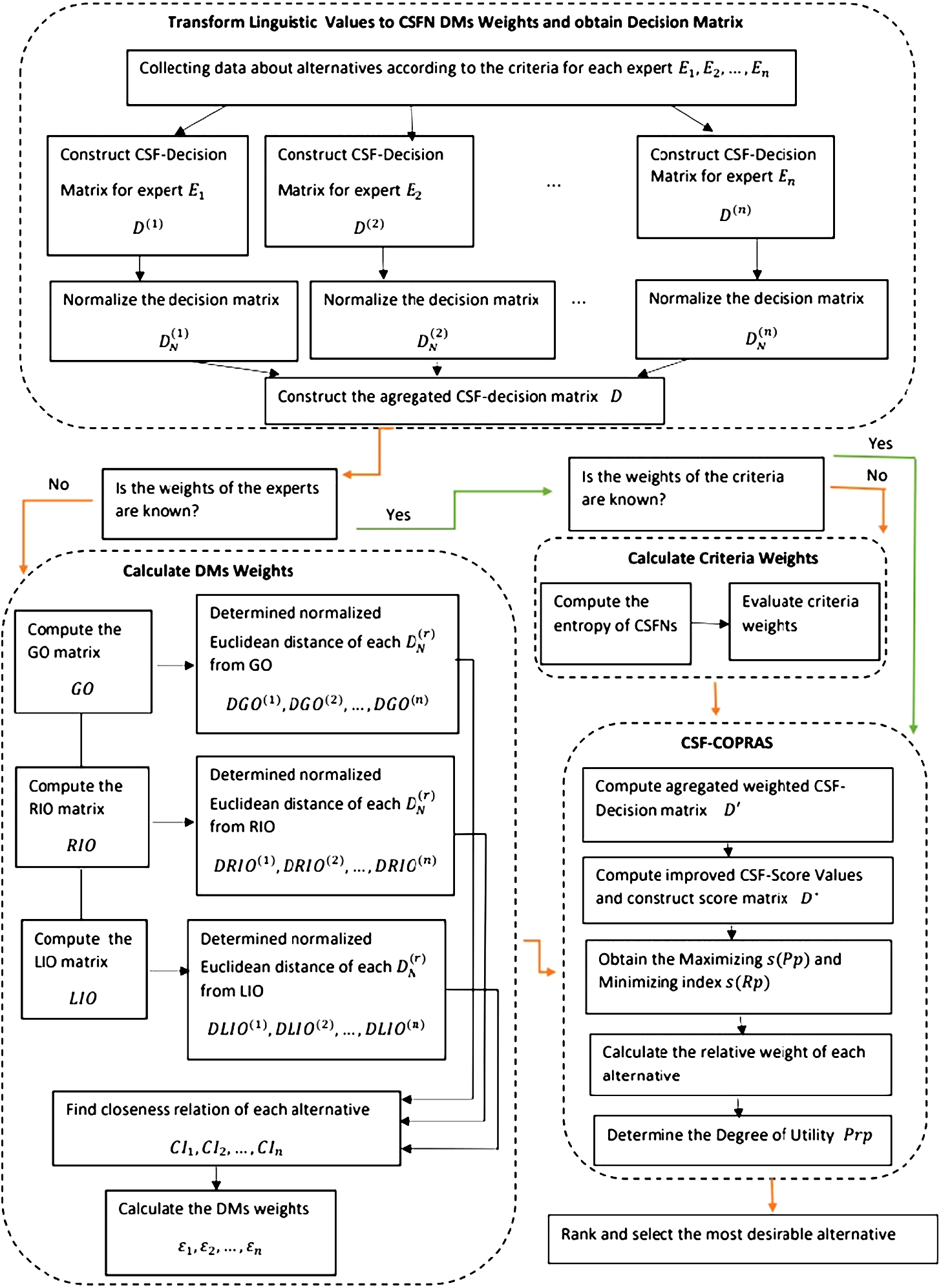
The procedure of the new COPRAS method based on entropy consists of the following steps:
Step I: Since the CSFDM may have some benefit and cost types criteria, as a first step, the information given by experts is normalized in the following way:
(2)
Step II: Consider the weights of the experts. There are two cases:
Case I: If the weights of experts are known, these values can be used. So this step is skipped.
Case II: If the weights of the experts are completely unknown, it is not possible to establish the final NCSFDM. So, the weights of the experts need to be determined. The weights of the experts are calculated in the following way:
I: As a first substep, the group opinion (GO) matrix is obtained by using the CSFWA operator of decision values in the NCSFDMs and the GO matrix is represented as follows:
II: Determine the right ideal opinion (RIO) matrix and left ideal opinion (LIO) matrix as follows:
III: By using the normalized Euclidean distance function, calculate the distances of each NCSFDMs
IV: The closeness indices (CI) (given by Yue, 2013) are calculated as follows:
(3)
V: The weights of experts are computed as follows:
(4)
Step III: The collective decision of all experts is obtained by merging the independent decision of each expert with their weights via CSFWA operator and the aggregated complex spherical fuzzy decision matrix (ACSFDM)
Step IV: Since the weight matrix of criteria shows the importance of each criterion, this matrix should be constructed. There are two cases:
Case I: If the weights of criteria are known, these values can be used. So this step is skipped.
Case II: If the weights of criteria are completely unknown, construct the weight matrix of the criteria from ACSFDM by using the entropy measure function. Let
(5)
Step V: Find the aggregated weighted complex spherical fuzzy decision matrix (AWCSFDM)
The
Step VI: Since the elements of the AWCSFDM
(6)
Step VII: Let
(7)
(8)
Step VIII: Calculate the relative weight of each alternative
(9)
Step IX: Determine the priority order
(10)
Step X: If
5An Illustrative Example
Suppliers have always been an integral component of a company’s management policy; however, the relationship between companies and their suppliers has traditionally been distant. In today’s global economy of just-in-time (JIT) manufacturing and value-added focus, there is a heightened need to change this adversarial relationship to one of cooperation and seamless integration. JIT requires the vendor to manufacture and deliver to the company the precise quantity and quality of material at the required time. Thus the performance of the supplier becomes a key element in a company’s success or failure. In order to attain the goals of low cost, consistently high quality, flexibility, and quick response, companies have increasingly considered better supplier selection approaches. These approaches require cooperation in sharing costs, benefits, and expertise in attempting to understand one another’s strengths and weaknesses, which in turn leads to single sourcing, supplier, and long-term partnerships. Since the supplier selection process encompasses different functions (such as purchasing, quality, production, etc.) within a company, it is a multi-objective problem, encompassing many tangible and intangible factors in a hierarchical manner. The evaluation of intangible factors requires the assessment of expert judgment, and the hierarchical structure requires decomposition and synthesis of these factors (Bhutta and Huq, 2002).
Now, we consider the problem “selection of the strategic supplier selection” given by Igoulalene et al. (2015) and solve this problem to demonstrate the applicability and effectiveness of the proposed method. In this problem, the stakeholders (DMs) evaluate the five suppliers given as
Table 5
Illustrative example (stakeholder preferences given in Igoulalene et al., 2015).
| G | VG | G | ||
| MG | G | MG | ||
| VG | G | VG | ||
| G | G | G | ||
| MG | G | M | ||
| M | MG | G | ||
| G | MG | MG | ||
| MG | M | MG | ||
| VG | VG | VG | ||
| VG | G | VG | ||
| VG | VG | G | ||
| VG | VG | G | ||
| MG | G | G | ||
| M | M | MG | ||
| VG | G | G | ||
| G | MG | MG | ||
| M | MG | MG | ||
| MP | M | M | ||
| G | G | MG | ||
| M | MG | M |
Table 6
CSFDMsestablished by expert
Table 7
CSFDMsestablished by expert
Table 8
CSFDMsestablished by expert
Table 9
NCSFDM of the expert
Table 10
NCSFDM of the expert
Table 11
NCSFDM of the expert
Table 12
GO matrices.
| GO | ||
Table 13
RIO matrices.
| RIO | ||
Step I: In this example,
Table 14
LIO matrices.
| LIO | ||
Step II: The objective weighs of experts are calculated using the following steps:
I: GO matrix is obtained using the CSFWA operator (Eq. (3)) and is shown in Table 12.
II: RIO and LIO matrices are shown in Tables 13 and 14.
III: DGO, DRIO and DLIO matrices are calculated using normalized Euclidean distance function and shown in Table 15.
IV: By using equation (3), we obtain the closeness indices as
Table 15
DGO, DRIO and DLIO matrices.
| DGO | |||||
| 0.1213 | 0.3204 | 0.1112 | 0.2494 | 0.2432 | |
| 0.2332 | 0.2106 | 0.1858 | 0.1538 | 0.1930 | |
| 0.1213 | 0.2587 | 0.2210 | 0.1856 | 0.2363 |
| DRIO | |||||
| 0.2766 | 0.4791 | 0.2171 | 0.3612 | 0.3175 | |
| 0.2171 | 0.4439 | 0.3070 | 0.3146 | 0.2277 | |
| 0.2766 | 0.3020 | 0.2171 | 0.2171 | 0.2695 |
| DLIO | |||||
| 0.2171 | 0.2774 | 0.3070 | 0.2171 | 0.2695 | |
| 0.2766 | 0.3497 | 0.2171 | 0.2805 | 0.4746 | |
| 0.2171 | 0.4727 | 0.3070 | 0.3612 | 0.3175 |
V: The weights of experts are found using equation (4) as
Step III: The ACSFDM is calculated by considering the CSFDMs, which are given in Table 9 and the ACSFDM is given in Table 16.
Step IV: The objective weights of the criteria are calculated by using the proposed entropy-based approach. First, the entropy value of each criterion is calculated by applying Eq. (2). Then entropy is used in Eq. (5) for obtaining objective weights of the criteria and these weights are given in Table 17.
Table 16
The ACSFDM.
| D | ||
Step V: After determining the weights of the criteria, the AWCSFDM
Table 17
Weights of criteria.
| ω | ||||
| 0.2802 | 0.4421 | 0.1876 | 0.3697 | |
| 0.7198 | 0.5578 | 0.8124 | 0.6303 | |
| 0.2646 | 0.2051 | 0.2986 | 0.2317 |
Step VI: Table 18 gives the aggregated scores of each alternative which are represented as CSFNs in the column. To calculate the real values, we defuzzify these CSFNs by using Eq. (6) and so, we obtain the score matrix as given in Table 19.
Table 18
The AWCSFDM.
Table 19
Score matrix
| 0.8919 | 0.5810 | 1.0357 | 0.4101 | |
| 0.6699 | 0.5376 | 0.7791 | 0.3996 | |
| 1.0191 | 0.7958 | 1.0412 | 0.4185 | |
| 0.7636 | 0.4468 | 0.9705 | 0.4131 | |
| 0.6032 | 0.4082 | 0.8401 | 0.3855 |
Step VII, VIII, IX, X: Using Eq. (7) and Eq. (8), calculate
Table 20
| Rank | |||||
| 0.8362 | 0.4101 | 1.2366 | 91.98 | 2 | |
| 0.6622 | 0.3996 | 1.0732 | 79.82 | 4 | |
| 0.9520 | 0.4185 | 1.3443 | 100 | 1 | |
| 0.7270 | 0.4131 | 1.1244 | 83.64 | 3 | |
| 0.6172 | 0.3855 | 1.0431 | 77.60 | 5 |
As a result, we can see that the order of ranking among seven alternatives is
6Comparative Analyses
6.1Comparison with Some Existing Methods in Different Set Theories
In this subsection, we give comparative studies with the F-TOPSIS developed by Igoulalene et al. (2015) and SF-COPRAS by Omerali and Kaya (2022) to demonstrate the accuracy of the proposed entropy based CSF-COPRAS method.
Igoulalene et al. (2015) solved the MCGDM problem about “selection of the strategic supplier” which consists of fuzzy values. For this problem, the authors have used the consensus based neat OWA and TOPSIS method to calculate the ranking of alternatives. They also have computed the weight of criteria objectively by using correlation coefficient and standard deviation method. In the previous section, we solved the same problem with our method and here we give the comparison by analysing the ranking result obtained from the F-TOPSIS method.
On the other hand, we consider the MCGDM problem about “selection of the augmented reality application” solved by Omerali and Kaya (2022). The authors solved this problem by applying the COPRAS method in the SF environment. The difference between this method and the method given Igoulalene et al. (2015) is that the weights of DMs and criteria were taken into subjectively. We also solve this problem by using the proposed method to show the comparison. We first convert the SF values in the problem “selection of the augmented reality application” given by Omerali and Kaya (2022) to the CSF values by taking the phase terms as zero and then we solve this problem by using the proposed method that allows to calculate the weights of criteria and experts objectively. We also note that when solving this problem, we take the criteria
Table 21
Comparison of the ranking of the results of problems given with different set theories.
| Problem of the select. of the strategic supplier | F-TOPSIS method given by Igoulalene et al. (2015) | The proposed entropy based CSF-COPRAS method |
| Used set theory | FS | CSFS |
| Weighting method | Subjective DM weighting Objective criteria weighting | Objective DM weighting Objective criteria weighting |
| Ranking results |
| Problem of the select. of the augmented reality application | SF-COPRAS method given by Omerali and Kaya (2022) | The proposed entropy based CSF-COPRAS method |
| Used set theory | SFS | CSFS |
| Weighting method | Subjective DM weighting Subjective criteria weighting | Objective DM weighting Objective criteria weighting |
| Ranking results |
6.2Comparison with Some Existing Methods in CSFS Theory
The second analysis aims to compare the proposed methods with the existing methods in CSF environment given by Zahid et al. (2022), Naeem et al. (2022) and Aydoğdu et al. (2023). We first remark on the characteristic properties of these methods in Table 22.
Table 22
Characteristic properties of the mentioned studies in CSF environment.
| Given by | Method | Obj. DMs weights | Obj. criteria weights |
| Zahid et al. (2022) | CSF-ELECTRE II | X | X |
| Naeem et al. (2022) | Based on aggregation op. | X | √ |
| Aydoğdu et al. (2023) | CSF-TOPSIS based on entropy | √ | √ |
As explained in Table 22, in the CSF-ELECTRE II method given by Zahid et al. (2022), both weights of DMs and criteria are taken as subjective. However, in the method based on aggregation operators presented by Naeem et al. (2022), the weights of criteria are calculated objectively by using the entropy measure function whereas the weights of DMs are subjective. In addition, in the CSF-TOPSIS based on entropy method given by (Aydoğdu et al., 2023), both the weights of DMs and criteria are calculated objectively. To compare the proposed method with the mentioned three methods, we consider the problems given in these studies and solve all of them by using the proposed method. As a result, we show the rankings in Table 23.
Table 23
Comparison of the ranking of the problems solved with CSF methods.
| Problem | Ranking given in related study | Ranking the proposed method |
| Select. of the tech. to treat cad.-contam. water (Zahid et al., 2022) | ||
| Green supplier selection (Naeem et al., 2022) | ||
| Select. of the advertisement on Facebook (Aydoğdu et al., 2023) |
Remark that the proposed method gives the same best alternatives as the other existing methods in the CSF environment. So it can be concluded that the proposed objective weighting method can work with the different MCDM/MCGDM approaches and the ranking results remain mostly the same.
6.3Sensitivity Analysis and Comparison of Entropies
In this subsection, we first analyse the consistency of the proposed method by calculating the criteria weights with the mentioned entropy measure functions. Then, we give a comparison between the entropy measures (
Sensitivity analysis: The entropy measures
Now, we apply these entropy measures to the problem “green supplier selection” to obtain the weights of criteria and then we show the weights of criteria in Fig. 3.
Fig. 3
Criteria weight under different entropies.
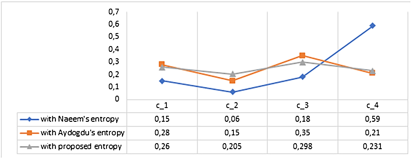
Table 24
Rankingresults under different entropies.
| Entropy | Given by | Ranking |
| Naeem et al. (2022) | ||
| Aydoğdu et al. (2023) | ||
| E | Proposed method |
Also, we present the results of the same problem under the proposed method with the existing and the novel entropy measure functions in Table 24. In conclusion, the same ranking results are found in each setting. This result shows the robustness and validity of the proposed entropy-based COPRAS method in the CSF environment.
Comparison of entropies: Based on the mathematical view and intuitive of human, if the inequality
(11)
Table 25
Entropy measure values.
| 0.7367 | 0.7886 | 1.0087 | 1.2325 | |
| 0.6952 | 0.7126 | 0.7149 | 0.7091 | |
| E | 0.9396 | 0.8997 | 0.8516 | 0.8163 |
According to Table 25, the values
6.4Discussion and Research Implications
Consequently, in Section 6.1, we compare some existing methods given in some different set theories with the proposed method and show the proposed method is consistent when both weights of criteria and DMs are calculated objectively. In Section 6.2, the proposed method is compared with the CSF-ELECTRE II method (given by Zahid et al., 2022) and CSF-TOPSIS based on entropy method (given by Aydoğdu et al., 2023) that calculates both weights of criteria and DMs objectively and also we compare the proposed method with the method based on aggregation operators (given by Naeem et al., 2022) that calculates these weights subjectively. These three methods were given in CSFS environment and so we can verify that the proposed method is stable since the best alternative is the same and the rankings are similar. Furthermore, one more confirmation to show the robustness and validity is obtained as a result of the obtained rankings by changing the entropy measure functions presented for sensitivity analysis in Section 6.3. Moreover, in this subsection, we show that the proposed entropy measure function is effective by comparing the other existing entropy measure functions. All these comparisons demonstrate that the proposed method has superiority in solving MCGDM problems by calculating the weights of criteria and DMs objectively in the CSF environment.
7Conclusion
CSF is a broader and more dominant model than the existing set theories since this theory does not only competently deal with two-dimensional information but also takes into account the doubtless and refusal part of the judgment as well as positive-membership and negative-membership. The main contribution of the study is the introduction of a novel improved COPRAS method under the CSF environment with unknown information about the DMs and criteria weights. In this study, the data of the weights of criteria and DMs are objectively determined. To obtain objective criteria weights, a new entropy measure is given on CSFs and the entropy weight model is developed. In order to eliminate the subjective collective information during the implementation of the method, the CSF-COPRAS method aggregates with the computed weights of the criteria weights of DMs to acquire the final alternative rank. Then, to explain and show the validity of the proposed method, a numerical example and comparative analyses are given. Moreover, the applied methods’ preference ranking of alternatives is compared with different MCDM and MCGDM approaches under different environments. The fact that the best alternative is the same in all compared methods showed that the entropy-based CSF-COPRAS method is quite robust. So, we have presented the proposed study as a more general model than all the compared studies and have explained its advantages with method analysis. For future work, we aim to investigate different types of entropy measure functions and apply these functions to the different types of traditional MCGDM methods such as WASPAS, AHP, SWAM, etc. Also, we plan to obtain some new kind of similarity measure for CSFs environment and further, we will research to find the applications areas of these approaches to real-life problems such as medical diagnosis, image detection and pattern recognition.
Acknowledgements
The authors are thankful to the editor and the anonymous referees for their valuable suggestions.
References
1 | Akram, M., Bashir, A., Garg, H. ((2020) ). Decision-making model under complex picture fuzzy Hamacher aggregation operators. Computational and Applied Mathematics, 39: (3), 1–38. |
2 | Akram, M., Kahraman, C., Zahid, K. ((2021) a). Extension of TOPSIS model to the decision-making under complex spherical fuzzy information. Soft Computing, 25: , 10771–10795. |
3 | Akram, M., Al-Kenani, A.N., Shabir, M. ((2021) b). Enhancing ELECTRE I method with complex spherical fuzzy information. International Journal of Computational Intelligence Systems, 14: (1), 1–31. |
4 | Akram, M., Kahraman, C., Zahid, K. ((2021) c). Group decision-making based on complex spherical fuzzy VIKOR approach. Knowledge-Based Systems, 216: , 106793. |
5 | Akram, M., Khan, A., Alcantud, J., Santos-García, G. ((2021) d). A hybrid decision-making framework under complex spherical fuzzy prioritized weighted aggregation operators. Expert Systems, 38: (6), e12712. |
6 | Aldemir, B., Güner, E., Aydoğdu, E., Aygün, H. ((2021) ). Complex spherical fuzzy TOPSIS method with Dombi aggregation operators. In: 1st International Symposium on Recent Advances in Fundamental and Applied Sciences. Ataturk University Publications. |
7 | Ali, Z., Mahmood, T., Yang, M. ((2020) ). TOPSIS method based on complex spherical fuzzy sets with Bonferroni mean operators. Mathematics, 8: (10), 1739–1760. |
8 | Alimardani, M., Hashemkhani Zolfani, S., Aghdaie, M.H., Tamošaitienė, J. ((2013) ). A novel hybrid SWARA and VIKOR methodology for supplier selection in an agile environment. Technological and Economic Development of Economy, 19: (3), 533–548. |
9 | Alkan, Ö., Albayrak, Ö.K. ((2020) ). Ranking of renewable energy sources for regions in Turkey by fuzzy entropy based fuzzy COPRAS and fuzzy MULTIMOORA. Renewable Energy, 162: , 712–726. |
10 | Alipour, M., Hafezi, R., Rani, P., Hafezi, M., Mardani, A. ((2021) ). A new Pythagorean fuzzy-based decision-making method through entropy measure for fuel cell and hydrogen components supplier selection. Energy, 234: , 121208. |
11 | Alkouri, A.U.M., Salleh, A.R. ((2013) ). Complex Atanassov’s intuitionistic fuzzy relation. Abstract and Applied Analysis, 2013: , 287382. |
12 | Anser, M.K., Mohsin, M., Abbas, Q., Chaudhry, I.S. ((2020) ). Assessing the integration of solar power projects: SWOT-based AHP–F-TOPSIS case study of Turkey. Environmental Science and Pollution Research, 27: (25), 31737–31749. |
13 | Atanassov, K. ((2003) ). Intuitionistic fuzzy sets. Fuzzy Sets and Systems, 20: (1), 87–96. |
14 | Aydoğdu, A., Gül, S. ((2020) ). A novel entropy proposition for spherical fuzzy sets and its application in multiple attribute decision-making. International Journal of Intelligent Systems, 35: (9), 1354–1374. |
15 | Aydoğdu, A., Gül, S. ((2022) ). New entropy propositions for interval-valued spherical fuzzy sets and their usage in an extension of ARAS (ARAS-IVSFS). Expert Systems, 39: (4), e12898. |
16 | Aydoğdu, E., Güner, E., Aldemir, B., Aygün, H. ((2023) ). Complex spherical fuzzy TOPSIS based on entropy. Expert Systems with Applications, 215: , 119331. |
17 | Azam, M., Ali Khan, M.S., Yang, S. ((2022) ). A decision-making approach for the evaluation of information security management under complex intuitionistic fuzzy set environment. Journal of Mathematics, 2022: , 9704466. |
18 | Balali, A., Valipour, A., Edwards, R., Moehler, R. ((2021) ). Ranking effective risks on human resources threats in natural gas supply projects using ANP-COPRAS method: case study of Shiraz. Reliability Engineering and System Safety, 208: , 107442. |
19 | Bozanic, D., Tešić, D., Milić, A. ((2020) ). Multicriteria decision making model with Z-numbers based on FUCOM and MABAC model. Decision Making: Applications in Management and Engineering, 3: (2), 19–36. |
20 | Brauers, W.K., Zavadskas, E.K. ((2006) ). The MOORA method and its application to privatization in a transition economy. Control and Cybernetics, 35: (2), 445–469. |
21 | Bhutta, K.S., Huq, F. ((2002) ). Supplier selection problem: a comparison of the total cost of ownership and analytic hierarchy process approaches. Supply Chain Management, 7: (3), 126–135. |
22 | Buyukozkan, G., Gocer, F. ((2019) ). A novel approach integrating AHP and COPRAS under Pythagorean fuzzy sets for digital supply chain partner selection. IEEE Transactions on Engineering Management, 68: (5), 1486–1503. |
23 | Chaurasiya, R., Jain, D. ((2022) ). Pythagorean fuzzy entropy measure-based complex proportional assessment technique for solving multi-criteria healthcare waste treatment problem. Granular Computing, 7: , 917–930. |
24 | Chen, S.M. ((1988) ). A new approach to handling fuzzy decision-making problems. IEEE Transactions on Systems, Man, and Cybernetics, 18: (6), 1012–1016. |
25 | Cuong, B. ((2013) ). Picture fuzzy sets-first results. Seminar on Neuro–Fuzzy Systems with Applications. Institute of Mathematics, Hanoi. |
26 | De Luca, A., Termini, S. ((1972) ). A definition of a nonprobabilistic entropy in the setting of fuzzy sets theory. Information and Control, 20: (4), 301–312. |
27 | De Luca, A., Termini, S. ((1977) ). On the convergence of entropy measures of a fuzzy set. Kybernetes, 6: (3), 219–227. |
28 | Diakoulaki, D., Mavrotas, G., Papayannakis, L. ((1995) ). Determining objective weights in multiple criteria problems: the CRITIC method. Computers and Operations Research, 22: (7), 763–770. |
29 | Dorfeshan, Y., Mousavi, S.M. ((2019) ). A group TOPSIS-COPRAS methodology with Pythagorean fuzzy sets considering weights of experts for project critical path problem. Journal of Intelligent and Fuzzy Systems, 36: (2), 1375–1387. |
30 | Ecer, F. ((2014) ). A hybrid banking websites quality evaluation model using AHP and COPRAS-G: a Turkey case. Technological and Economic Development of Economy, 20: (4), 758–782. |
31 | Fan, J., Xie, W. ((1999) ). Distance measure and induced fuzzy entropy. Fuzzy Sets and Systems, 104: (2), 305–314. |
32 | Gupta, H., Barua, M.K. ((2017) ). Supplier selection among SMEs on the basis of their green innovation ability using BWM and fuzzy TOPSIS. Journal of Cleaner Production, 152: , 242–258. |
33 | Gül, S., Aydoğdu, A. ((2021) ). Novel entropy measure definitions and their uses in a modified combinative distance-based assessment (CODAS) method under picture fuzzy environment. Informatica, 32: (4), 759–794. |
34 | Güner, E., Aygün, H. ((2020) ). Generalized spherical fuzzy Einstein aggregation operators: application to multi-criteria group decision-making problems. Conference Proceedings of Science and Technology, 3: (2), 227–235. |
35 | Güner, E., Aygün, H. ((2022) ). Spherical fuzzy soft sets: theory and aggregation operator with its applications. Iranian Journal of Fuzzy Systems, 19: (2), 83–97. |
36 | Güner, E., Aldemir, B., Aydoğdu, E., Aygün, H. (2022). Spherical fuzzy sets: AHP-COPRAS method based on Hamacher aggregation operator. Studies on Scientific Developments in Geometry, Algebra, and Applied Mathematics. |
37 | Hung, W., Yang, M. ((2006) ). Fuzzy entropy on intuitionistic fuzzy sets. International Journal of Intelligent Systems, 21: (4), 443–451. |
38 | Hwang, C.-L., Yoon, K. ((1981) ). Methods for multiple attribute decision making. In: Multiple Attribute Decision Making, Lecture Notes in Economics and Mathematical Systems, Vol. 186: . Springer, Berlin, Heidelberg, pp. 58–191. |
39 | Igoulalene, I., Benyoucef, L., Tiwari, M.K. ((2015) ). Novel fuzzy hybrid multi-criteria group decision making approaches for the strategic supplier selection problem. Expert Systems with Applications, 42: (7), 3342–3356. |
40 | Kahraman, C., Onar, S.C., Öztayşi, B., Şeker, Ş., Karaşan, A. ((2020) ). Integration of fuzzy AHP with other fuzzy multicriteria methods: a state of the art survey. Journal of Multiple-Valued Logic and Soft Computing, 35: (1–2), 61–92. |
41 | Keršuliene, V., Zavadskas, E.K., Turskis, Z. ((2010) ). Selection of rational dispute resolution method by applying new step-wise weight assessment ratio analysis (SWARA). Journal of Business Economics and Management, 11: (2), 243–258. |
42 | Keshavarz-Ghorabaee, M. ((2021) ). Assessment of distribution center locations using a multi-expert subjective–objective decision-making approach. Scientific Reports, 11: (1), 1–19. |
43 | Keshavarz-Ghorabaee, M., Amiri, M., Kazimieras Zavadskas, E., Antuchevičienė, J. ((2017) ). Assessment of third-party logistics providers using a CRITIC–WASPAS approach with interval type-2 fuzzy sets. Transport, 32: (1), 66–78. |
44 | Keshavarz-Ghorabaee, M., Amiri, M., Zavadskas, E.K., Turskis, Z., Antucheviciene, J. ((2021) ). Determination of objective weights using a new method based on the removal effects of criteria (MEREC). Symmetry, 13: (4), 525. |
45 | Kumari, R., Mishra, A.R. ((2020) ). Multi-criteria COPRAS method based on parametric measures for intuitionistic fuzzy sets: application of green supplier selection. Iranian Journal of Science and Technology, Transactions of Electrical Engineering, 44: (4), 1645–1662. |
46 | Lu, J., Zhang, S., Wu, J., Wei, Y. ((2021) ). COPRAS method for multiple attribute group decision making under picture fuzzy environment and their application to green supplier selection. Technological and Economic Development of Economy, 27: (2), 369–385. |
47 | Mahmood, T., Kifayat, U., Khan, Q., Jan, N. ((2018) ). An approach toward decision making and medical diagnosis problems using the concept of spherical fuzzy sets. Neural Computing and Applications, 31: , 7041–7053. |
48 | Maji, P.K., Biswas, R., Roy, A.R. ((2001) ). Fuzzy soft sets. Journal of Fuzzy Mathematics, 9: (3), 589–602. |
49 | Mishra, A.R., Rani, P., Pandey, K., Mardani, A., Streimikis, J., Streimikiene, D., Alrasheedi, M. ((2020) ). Novel multi-criteria intuitionistic fuzzy SWARA-COPRAS approach for sustainability evaluation of the bioenergy production process. Sustainability, 12: (10), 4155. |
50 | Mishra, A.R., Saha, A., Rani, P., Hezam, I.M., Shrivastava, R., Smarandache, F. ((2022) ). An integrated decision support framework using single-valued-MEREC-MULTIMOORA for low carbon tourism strategy assessment. IEEE Access, 10: , 24411–24432. |
51 | Naeem, M., Qiyas, M., Botmart, T., Abdullah, S., Khan, N. ((2022) ). Complex spherical fuzzy decision support system based on entropy measure and power operator. Journal of Function Spaces, 2022: , 1–25. |
52 | Omerali, M., Kaya, T. ((2022) ). Augmented reality application selection framework using spherical fuzzy COPRAS multi criteria decision making. Cogent Engineering, 9: (1), 220610. |
53 | Opricovic, S. ((1998) ). Multicriteria Optimization of Civil Engineering Systems. PhD Thesis, Faculty of Civil Engineering, Belgrade, 302 pp. |
54 | Pamucar, D., Stević, Ž., Sremac, S. ((2018) ). A new model for determining weight coefficients of criteria in MCDM models: full consistency method (FUCOM). Symmetry, 10: (9), 393. |
55 | Pamucar, D., Deveci, M., Canıtez, F., Lukovac, V. ((2020) ). Selecting an airport ground access mode using novel fuzzy LBWA-WASPAS-H decision making model. Engineering Applications of Artificial Intelligence, 93: , 103703. |
56 | Pamucar, D., Ecer, F., Deveci, M. ((2021) ). Assessment of alternative fuel vehicles for sustainable road transportation of United States using integrated fuzzy FUCOM and neutrosophic fuzzy MARCOS methodology. Science of The Total Environment, 788: , 147763. |
57 | Peng, X., Zhang, X., Luo, Z. ((2020) ). Pythagorean fuzzy MCDM method based on CoCoSo and CRITIC with score function for 5G industry evaluation. Artificial Intelligence Review, 53: (5), 3813–3847. |
58 | Rani, P., Mishra, A.R., Krishankumar, R., Mardani, A., Cavallaro, F., Soundarapandian Ravichandran, K., Balasubramanian, K. ((2020) a). Hesitant fuzzy SWARA-complex proportional assessment approach for sustainable supplier selection (HF-SWARA-COPRAS). Symmetry, 12: (7), 1152. |
59 | Rani, P., Mishra, A.R., Mardani, A. ((2020) b). An extended Pythagorean fuzzy complex proportional assessment approach with new entropy and score function: application in pharmacological therapy selection for type 2 diabetes. Applied Soft Computing, 94: , 106441. |
60 | Rani, P., Mishra, A.R., Saha, A., Hezam, I.M., Pamucar, D. ((2022) ). Fermatean fuzzy Heronian mean operators and MEREC-based additive ratio assessment method: an application to food waste treatment technology selection. International Journal of Intelligent Systems, 37: (3), 2612–2647. |
61 | Ramot, D., Milo, R., Friedman, M., Kandel, A. ((2002) ). Complex fuzzy sets. IEEE Transactions on Fuzzy Systems, 10: (2), 171–186. |
62 | Ramot, D., Friedman, M., Langholz, G., Kandel, A. ((2003) ). Complex fuzzy logic. IEEE Transactions on Fuzzy Systems, 11: (4), 450–461. |
63 | Rezaei, J. ((2015) ). Best-worst multi-criteria decision-making method. Omega, 53: , 49–57. |
64 | Saaty, T.L. ((1980) ). How to make a decision: the analytic hierarchy process. European Journal of Operational Research, 48: (1), 9–26. |
65 | Saaty, T.L. ((1996) ). Decision with the Analytic Network Process. University of Pittsburgh, USA. |
66 | Sakthivel, G., Ilangkumaran, M., Gaikwad, A. ((2015) ). A hybrid multi-criteria decision modeling approach for the best biodiesel blend selection based on ANP-TOPSIS analysis. Ain Shams Engineering Journal, 6: (1), 239–256. |
67 | Schitea, D., Deveci, M., Bilgili, K. ((2019) ). Hydrogen mobility roll-up site selection using intuitionistic fuzzy sets based WASPAS, COPRAS and EDAS. International Journal of Hydrogen Energy, 44: (16), 8585–8600. |
68 | Thaoa, N., Smarandache, F. ((2019) ). A new fuzzy entropy on Pythagorean fuzzy sets. Journal of Intelligent and Fuzzy Systems, 37: , 1065–1074. |
69 | Torkayesh, A.E., Pamucar, D., Ecer, F., Chatterjee, P. ((2021) ). An integrated BWM-LBWA-CoCoSo framework for evaluation of healthcare sectors in Eastern Europe. Socio-Economic Planning Sciences, 78: , 101052. |
70 | Ullah, K., Mahmood, T., Ali, Z., Jan, N. ((2020) ). On some distance measures of complex Pythagorean fuzzy sets and their applications in pattern recognition. Complex and Intelligent Systems, 6: (1), 15–27. |
71 | Xuecheng, L. ((1992) ). Entropy, distance measure and similarity measure of fuzzy sets and their relations. Fuzzy Sets and Systems, 52: (3), 305–318. |
72 | Yager, R. ((2013) ). Pythagorean fuzzy subsets. In: Proceedings of Joint IFSA World Congress and NAFIPS Annual Meeting, Edmonton, Canada. |
73 | Yang, Y.P.O., Shieh, H.M., Leu, J.D., Tzeng, G.H. ((2008) ). A novel hybrid MCDM model combined with DEMATEL and ANP with applications. International Journal of Operations Research, 5: (3), 160–168. |
74 | Yue, Z. ((2013) ). An avoiding information loss approach to group decision making. Applied Mathematical Modelling, 37: (1–2), 112–126. |
75 | Zadeh, L. ((1965) ). Fuzzy sets. Information and Control, 8: , 338–353. |
76 | Zahid, K., Akram, M., Kahraman, C. ((2022) ). A new ELECTRE-based method for group decision-making with complex spherical fuzzy information. Knowledge-Based Systems, 243: , 1–25. |
77 | Zavadskas, E.K., Kaklauskas, A., Sarka, V. ((1994) ). The new method of multicriteria complex proportional assessment of projects. Technological and Economic Development of Economy, 1: (3), 131–139. |
78 | Žižović, M., Pamucar, D. ((2019) ). New model for determining criteria weights: Level Based Weight Assessment (LBWA) model. Decision Making: Applications in Management and Engineering, 2: (2), 126–137. |


