
Circular Intuitionistic Fuzzy ELECTRE III Model for Group Decision Analysis
Abstract
ELECTRE III is a well-established outranking relation model used to address the ranking of alternatives in multi-criteria and multi-actor decision-making problems. It has been extensively studied across various scientific fields. Due to the complexity of decision-making under uncertainty, some higher-order fuzzy sets have been proposed to effectively model this issue. Circular Intuitionistic Fuzzy Set (CIFS) is one such set recently introduced to handle uncertain IF values. In CIFS, each element of the set is characterized by a circular area with a radius, r and membership/non-membership degrees as the centre. This paper introduces CIF-ELECTRE III, an extension of ELECTRE III within the CIFS framework, for group decision analysis. To achieve this, we define extensions for the group decision matrix and group weighting vector based on CIFS conditions, particularly focusing on optimistic and pessimistic attitudes. These attitudinal characters of the group of actors are constructed using conditional rules to ensure that each element of the set falls within the circular area. Parameterized by
1Introduction
Decision theory is a rapidly evolving field, particularly in the context of multi-criteria and multi-actor (or group) decision-making processes. This process entails ranking, selecting, or assigning a set of alternatives that are evaluated based on several conflicting criteria, typically performed by a group of individuals. The input data for this procedure can originate from various types of information, including quantitative and qualitative data. In many cases, this information may be subject to imprecision, ambiguity, or uncertainty due to measurement errors, imperfect knowledge, subjectivity, and other factors. Consequently, many decision-making models in the literature have been proposed to incorporate fuzzy set (FS) theory as a means of addressing this issue (Zadeh, 1965). In FS, each element of a set is characterized by a membership degree with a value in the unit interval
In some other studies, researchers have argued that there are cases that go beyond the complementary nature of membership and non-membership degrees, involving indeterminate or incomplete information. Atanassov (1986) introduced intuitionistic fuzzy set (IFS) as an extension of FS, where membership and non-membership degrees can exist independently within the unit interval, and the sum of the two degrees can be less than one. Additionally, a hesitancy degree was introduced to complement the membership and non-membership degrees. Similarly, IFS has undergone several developments, including the proposal of interval-valued IFS (IVIFS) (Atanassov and Gargov, 1989), type-2 IFS (T2IFS) (Zhao and Xiao, 2012), hesitant IFS (HIFS) (Beg and Rashid, 2014), among others, to represent uncertain membership and non-membership degrees (i.e. IF values). A substantial body of literature has reported on the expansion of multi-criteria and multi-actor decision-making models using these sets (Yusoff et al., 2011; Taib et al., 2016; Ecer et al., 2022).
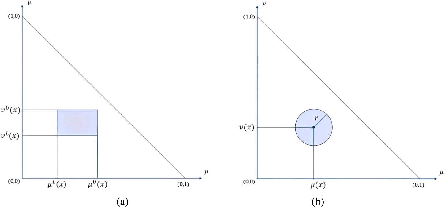
Recently, Atanassov (2020) introduced another extension of IFS, aiming to enhance the flexibility in interpreting and representing IF values. This extension is known as a Circular Intuitionistic Fuzzy Set (CIFS). In CIFS, each element of a set is characterized as a circle, with membership and non-membership degrees determining the centre and radius, denoted as r, which represents the region of uncertainty. The primary distinction between CIFS and IVIFS lies in their representation of imprecision. IVIFS is depicted as a rectangle (bounded by lower and upper bounds of membership and non-membership degrees) within the IFS interpretation triangle (IFIT). In contrast, CIFS expresses its uncertainty region with equidistant boundaries from the centre. Fig. 1 provides a geometrical interpretation of IVIFS and CIFS.
Fig. 1
Geometrical interpretation of (a) IVIFS and (b) CIFS.
The development of the CIFS theory is still in its early stages, and therefore, limited research has been conducted on it. In the initial paper, Atanassov (2020) introduced CIFS, along with some fundamental operations and relations, where the radius was confined to the range of
One of the intriguing developments in the context of CIFS in group decision-making problem was introduced by Kahraman and Alkan (2021). Specifically, they proposed the inclusion of psychological behaviours within TOPSIS model under the CIFS environment, known as CIF-TOPSIS. These characteristics involve optimistic and pessimistic attitudes, which are represented as IF values derived from CIF values. The optimistic value is defined as the sum of the membership degree and the subtraction of the non-membership degree, both adjusted by the radius, r. Conversely, the pessimistic value is defined in the opposite manner. In general, the optimistic value reflects the group’s inclination toward higher membership degrees (validity), while the pessimistic value indicates a tendency toward higher non-membership degrees (non-validity). However, these operations have shown certain limitations. Specifically, they may result in optimistic and pessimistic values falling outside the circular area. Ideally, all values should remain within the circular region to accurately represent the data. Furthermore, Kahraman and Alkan (2021) restricted the radius, r to the range
In addition to the models mentioned above, ELECTRE (ELimination Et Choix Traduisant la REalité – elimination and choice expressing reality) is another well-established approach for handling multi-criteria and multi-actor decision-making problems. It was developed in the late 1960 by Roy (1968). ELECTRE is a comprehensive outranking relation model with several variants designed for different decision problems, including ranking, selection, and assignment of alternatives. These variants include ELECTRE I (Roy, 1968), ELECTRE II (Roy and Bertier, 1973), ELECTRE III (Roy, 1978), ELECTRE IV (Hugonnard and Roy, 1982), and more. Numerous studies have explored the use of ELECTRE models based on fuzzy concepts and their development, including their application in FS (Mohamadghasemi et al., 2020), IFS (Rouyendegh, 2017; Qu et al., 2018). Notably, ELECTRE III, which relies on fuzzy outranking relations, has been widely utilized for its effectiveness in the ranking process. Numerous developments related to FS, IFS, and IVFS have been documented in the literature (Joshi, 2016; Hashemi et al., 2016; Peng et al., 2019; Ramya et al., 2023; Forestal and Pi, 2022). To the best of our knowledge, there has been no study proposing the integration of CIFS into ELECTRE models, particularly ELECTRE III.
Given the aforementioned limitations and research gaps, the research contribution of this paper is to achieve the following main objectives.
1. To explore the CIFS theory and integrate it with the ELECTRE III model for group decision analysis, extending the model’s capabillities.
2. To redefine the operations used to generate optimistic and pessimistic IF values from the group decision matrix and group weighting vector. Additionally, suggest conditional rules to ensure that every element of the set remains within the circular area.
3. To demonstrate the applicabillity of the proposed model through a case study of stock-picking process.
4. To conduct a comprehensive comparative analysis with existing models and then justify sensitivity analyses to explore the impact of α-values, which reflect the linear combination of optimistic and pessimistic attitudes, criteria weights, and thresholds.
The remainder of this paper is structured as follows: Section 2 provides fundamental definitions and insights into IFS, CIFS, and ELECTRE III to clarify the proposed approach. In Section 3, we present a method for converting the group decision matrix and group weighting vector, based on CIF values, into optimistic and pessimistic forms of IF values. Section 4 introduces the proposed CIF-ELECTRE III model. We illustrate the application of this model with a numerical example in the context of stock selection in Section 5. Section 6 covers sensitivity analyses and a comparative discussion. In the conclusion (Section 7), we offer recommendations for future research.
2Preliminaries
This section recalls some basic definitions and related concepts of IFS, CIFS, and ELECTRE III model prior to the development of the proposed CIF-ELECTRE III.
2.1Intuitionistic Fuzzy Set
Definition 1
Definition 1(Atanassov, 1986).
Let X be a finite non-empty set. An Intuitionistic Fuzzy Set A (denoted IFS A) in X is defined as:
(1)
Several metric methods in terms of score and accuracy functions have been presented to compare two or more IF values (see, for example, Garg, 2016). The formal definition of these functions is given as the following. For brevity, the notation
Definition 2
Definition 2(Chen and Tan, 1994; Xu, 2007).
For IFS A, let
(2)
(3)
Moreover, let A and B be two IF values, then relations of score function and accuracy functions between A and B can be given as follows:
1. If
2. If
a. if
b. if
2.2Circular Intuitionistic Fuzzy Set
Definition 3
Definition 3(Atanassov, 2020).
Let X be a finite non-empty set. A Circular Intuitionistic Fuzzy Set
(4)
Similarly, the hesitancy function
Let
(5)
Remark 1.
Note that Definition 3 with radius
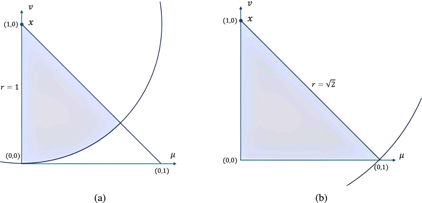
Recently, Atanassov and Marinov (2021) expanded the radius to
Fig. 2
Geometrical interpretation of CIFS for (a)
Two different ways for constructing of CIFSs have been proposed recently (Atanassov, 2020): i) based on the geometrical interpretations of the standard IFSs (Atanassova, 2010), and ii) based on hesitant IFS (Torra, 2010; Chen et al., 2016). In the following, the algorithm for building the CIFS from IFSs is presented.
Definition 4
Definition 4(Atanassov, 2020).
Let
(6)
(7)
(8)
The above expressions, under the group decision setting, can simply be assumed as the aggregated values of a group of actors
Definition 5
Definition 5(Kahraman and Alkan, 2021).
Let
(9)
(10)
Remark 2.
Note that Definition 5 has a limitation as these optimistic and pessimistic IF values are not within the circular area (or radius r) in the IFS triangle.
For example, the distance between the optimistic value and the centre of CIF value is obtained as:
2.3ELECTRE III Model
ELECTRE III is a preference model for ranking purposes. In a general case, it is used for multi-criteria decision-making problem (single actor). However, it also can be directly extended to the case of multi-actor (or group) problem. The following are the important notations related to the basic data and the construction of ELECTRE III model.
Let
Moreover, under the group decision setting, let
The main feature of ELECTRE III compared to the other variants of ELECTRE family is a type of preference so-called pseudo-criterion. Pseudo-criterion is a multilevel threshold approach, as can be defined in the following.
Definition 6
Definition 6(Roy and Vincke, 1984).
A pseudo-criterion is a function
The main process in ELECTRE III is the pairwise comparison of alternatives with respect to each criterion. These pairwise comparisons are presented in concordance and discordance indices. The concordance index
(11)
(12)
(13)
(14)
(15)
3Group Decision Matrix and Group Weighting Vector Based on CIFS
This section is devoted to the conversion of group decision matrix and group weighting vector to optimistic and pessimistic forms. In the previous work, Kahraman and Alkan (2021) proposed the formulation in Eqs. (9) and (10) to transform the CIF value to optimistic and pessimistic IF values, respectively. However, as stated in Remark 2, these values are not within the circular area of radius r in the IFS interpretation triangle. Hence, this formulation needs to be redefined. In the following, the definitions of group decision matrix and group weighting vector based on CIFS and their conversion to optimistic and pessimistic IF values are presented.
Definition 7.
Let
(16)
Upon checking the above definition,
Based on the Definiton 7, the concept of optimistic and pessimistic for weighting vector can be defined accordingly.
Definition 8.
Let
(17)
Likewise, the condition for standard IFS is fulfilled for
Fig. 3
Comparison of optimistic-pessimistic IF values for the proposed approach and Kahraman and Alkan’s approach.
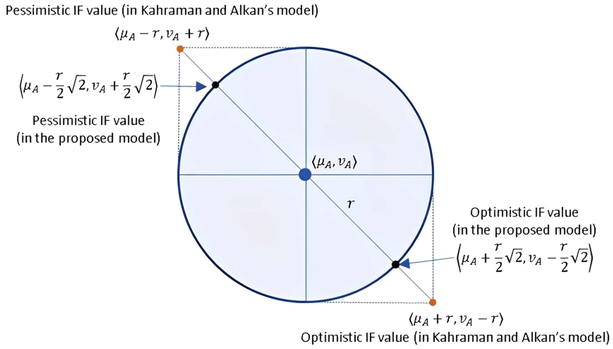
Moreover, it can easily be shown that the distance between the optimistic IF value,
Analogously, it can be shown for
Case (1): there is a possibility that
For example,
Case (2): there is possibility that
For example,
Fig. 4
Special cases for optimisitic decision element, when (a)
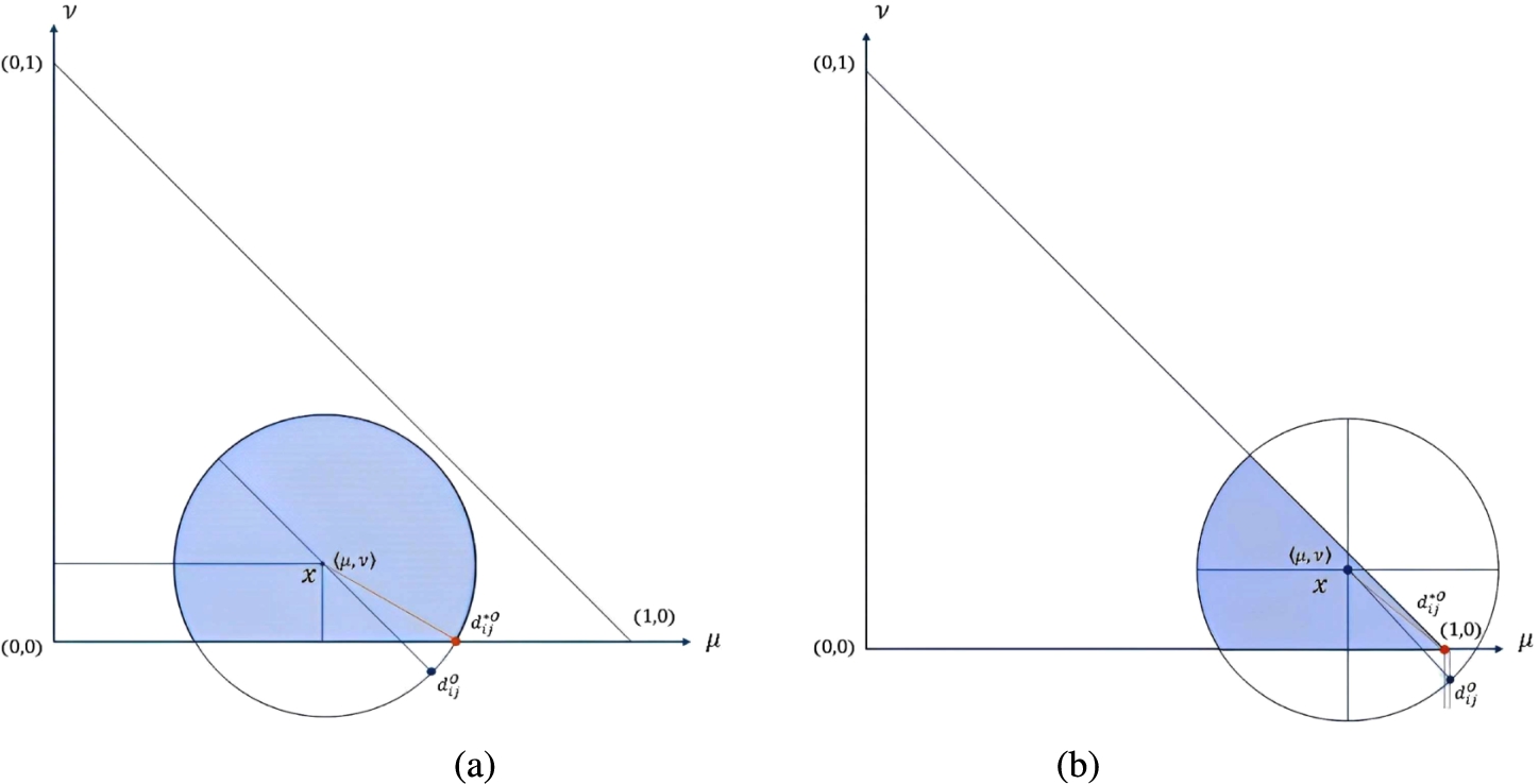
This leads to the following theorems for the elements of
Theorem 1.
Let
1. If
2. If
Proof.
It is clear that, for
(18)
(19)
For
Theorem 2.
Let
1. If
2. If
Proof.
For
(20)
(21)
For
Theorem 3.
Let
1. If
2. If
3. If
Proof.
The proof of this theorem is straightforward based on proofs of Theorem 1 and Theorem 2 with some adjustments. Instead of matrix, here vector is considered. □
The final outranking procedure in the CIF-ELECTRE III model is significantly influenced by the aformentioned definitions and theorems. For both the optimistic and pessimistic scenarios, separate scores underlie the ranking process. After identifying the optimistic and pessimistic scores, the composite ratio is defined. This ratio parameterizes the attitudinal character of the group of actors in order to determine the final score before the ranking process.
Definition 9.
Let
(22)
At the end, this composite ratio,
4CIF-ELECTRE III Model for Group Decision Analysis
Fig. 5
Framework of CIF-ELECTRE III.
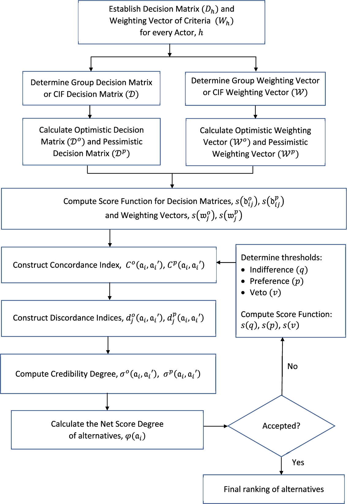
In this section, a novel CIF-ELECTRE III is presented. The framework of the proposed model is demonstrated in Fig. 5. The algorithm of the CIF-ELECTRE III is detailed in the following steps.
Step 1: Determine the list of potential alternatives, criteria, and actors to be implemented in the developed model. Let
Step 2: Generate the decision matrix
Step 3: Calculate the CIF decision matrix
Step 4: Calculate the optimistic decision matrix
Step 5: Calculate the deterministic form of optimistic decision matrix
Step 6: Next, determine the weighting vector of criteria for each actor
Step 7: Calculate the optimistic weighting vector
Step 8: Construct the optimistic concordance index
Step 9: Determine the optimistic discordance index
Step 10: Compute the credibility matrix
Step 11: Finally, calculate the net score degree (i.e. a composite ratio score) using Eq. (22), where the optimistic score degree
(23)
(24)
5Numerical Example
As a case study of the stock-picking process, this section shows how the suggested strategy was put into practice. Specifically, an investor intends to invest in one of the pre-screened stocks in Bursa Malaysia (i.e. under the technology sector). To finalize the decision, a set of criteria based on the fundamental analysis is considered for the further appraisal of stocks, i.e. using the forward-looking scenario analysis. The details of the decision-making process are demonstrated as follows.
Three financial analysts
Initially, using the predetermined linguistic scale such in Table 1(a), each analyst was asked to provide his/her preferences for all alternatives according to each criterion. The decision matrix of the performance rating by analysts is shown in Table 2.
Table 1
Linguistic scale for (a) rating of alternatives and (b) weighting of criteria.
| Linguistic terms | IFVs for alternatives | |
| m | n | |
| VVG/VVH | 0.9 | 0.1 |
| VG/VH | 0.7775 | 0.0625 |
| G/H | 0.6775 | 0.1625 |
| MG/MH | 0.5775 | 0.2625 |
| F/M | 0.4775 | 0.3635 |
| MB/ML | 0.3775 | 0.4625 |
| B/L | 0.2188 | 0.5438 |
| VB/VL | 0.0688 | 0.6938 |
| VVB/VVL | 0.1 | 0.9 |
| (a) | ||
| Linguistic terms | IFVs for alternatives | |
| m | n | |
| VI | 0.9 | 0.1 |
| I | 0.5813 | 0.1058 |
| M | 0.3313 | 0.3563 |
| U | 0.1813 | 0.5063 |
| VU | 0.1 | 0.9 |
| (b) | ||
Table 2
Linguistic decision matrix for each analyst.
| Criteria | Decision makers | |||||
| VG | MG | VG | F | B | ||
| VG | G | VG | MB | B | ||
| G | MG | VG | F | B | ||
| VG | VG | MG | MB | B | ||
| G | VG | G | F | F | ||
| MG | VG | MG | MG | B | ||
| G | F | VG | F | F | ||
| F | G | VVG | MG | MG | ||
| G | MG | VG | F | MG | ||
| F | G | MG | G | F | ||
| F | VG | VG | F | MG | ||
| F | G | G | F | G |
At this stage, the linguistic data provided by analysts are converted to their corresponding IF values to compute the group decision matrix
Table 3
Group decision matrix
Table 4
Optimistic decision matrix,
| Optimistic decision matrix, | Pessimistic decision matrix, | |||||||
From the group decision matrix (Table 3),
Table 5
Indifferent, preference and veto thresholds.
| q | L | L | M | M |
| p | MH | ML | MH | H |
| v | VH | H | VH | VH |
Table 6
Deterministic format of optimistic-pessimistic decision matrix and thresholds.
| 0.782 | 0.715 | 0.648 | 0.115 | 0.515 | 0.315 | 0.115 | 0.115 | |
| 0.515 | 0.715 | 0.515 | 0.715 | 0.248 | 0.715 | 0.115 | 0.448 | |
| 0.715 | 0.515 | 0.715 | 0.715 | 0.715 | 0.248 | 0.715 | 0.315 | |
| 0.191 | 0.347 | 0.315 | 0.515 | −0.085 | −0.085 | 0.048 | −0.018 | |
| −0.325 | 0.120 | 0.382 | 0.515 | −0.325 | −0.476 | 0.115 | 0.115 | |
| q | −0.325 | −0.325 | 0.115 | 0.115 | −0.325 | −0.325 | 0.115 | 0.115 |
| p | 0.315 | −0.085 | 0.315 | 0.515 | 0.315 | −0.085 | 0.315 | 0.515 |
| v | 0.715 | 0.515 | 0.715 | 0.715 | 0.715 | 0.515 | 0.715 | 0.715 |
Table 7
Linguistic preferences for criteria weights provided by analysts.
| VI | I | I | U | |
| VI | I | M | M | |
| I | I | I | U |
Table 8
Optimistic weight and pessimistic weight for criteria.
| (0.794,0.102;0.213) | (0.581,0.106;0) | (0.498,0.189;0.236) | (0.231,0.456;0.141) | |
| (0.98,0) | (0.581,0.106) | (0.665,0.02) | (0.33,0.355) | |
| (0.643,0.252) | (0.581,0.106) | (0.331,0.356) | (0.131,0.556) | |
| 0.99 | 0.738 | 0.821 | 0.487 | |
| 0.696 | 0.738 | 0.488 | 0.287 |
After that, determine the optimistic concordance index
Table 9
Optimistic and pessimistic concordance indices.
| 1 | 0.567 | 0.581 | 0.886 | 0.886 | 1 | 0.566 | 0.159 | 1 | 1 | ||
| 0.431 | 1 | 0.491 | 1 | 1 | 0.709 | 1 | 0.464 | 1 | 1 | ||
| 0.557 | 0.693 | 1 | 0.873 | 1 | 0.604 | 0.66 | 1 | 1 | 1 | ||
| 0.161 | 0.282 | 0.126 | 1 | 0.869 | 0.345 | 0.236 | 0.059 | 1 | 0.952 | ||
| 0.226 | 0.372 | 0.126 | 0.431 | 1 | 0.351 | 0.280 | 0.103 | 0.388 | 1 |
Table 10
Optimistic discordance indices for each criterion.
| Criteria 1 | Criteria 2 | Criteria 3 | Criteria 4 | |||||||||||||||||
| 1 | 0 | 0 | 0 | 0 | 1 | 0 | 0 | 0 | 0 | 1 | 0 | 0 | 0 | 0 | 1 | 0.425 | 0.425 | 0 | 0 | |
| 0 | 1 | 0 | 0 | 0 | 0 | 1 | 0 | 0 | 0 | 0 | 1 | 0 | 0 | 0 | 0 | 1 | 0 | 0 | 0 | |
| 0 | 0 | 1 | 0 | 0 | 0 | 0 | 1 | 0 | 0 | 0 | 0 | 1 | 0 | 0 | 0 | 0 | 1 | 0 | 0 | |
| 0.713 | 0.046 | 0.546 | 1 | 0 | 0.713 | 0.046 | 0.546 | 1 | 0 | 0.046 | 0 | 0.213 | 1 | 0 | 0 | 0 | 0 | 1 | 0 | |
| 1 | 1 | 1 | 0.479 | 1 | 1 | 1 | 1 | 0.479 | 1 | 0 | 0 | 0.046 | 0 | 1 | 0 | 0 | 0 | 0 | 1 | |
Table 11
Pessimistic discordance indices for each criterion.
| Criteria 1 | Criteria 2 | Criteria 3 | Criteria 4 | ||||||||||||||||
| 1 | 0 | 0 | 0 | 0 | 1 | 0.808 | 0.059 | 0 | 0 | 1 | 0 | 0.713 | 0 | 0 | 1 | 0 | 0 | 0 | 0 |
| 0 | 1 | 0.379 | 0 | 0 | 0 | 1 | 0 | 0 | 0 | 0 | 1 | 0.713 | 0 | 0 | 0 | 1 | 0 | 0 | 0 |
| 0 | 0 | 1 | 0 | 0 | 0.253 | 0.919 | 1 | 0 | 0 | 0 | 0 | 1 | 0 | 0 | 0 | 0 | 1 | 0 | 0 |
| 0.713 | 0.046 | 1 | 1 | 0 | 0.808 | 1 | 0.697 | 1 | 0 | 0 | 0 | 0.879 | 1 | 0 | 0 | 0 | 0 | 1 | 0 |
| 1 | 0.646 | 1 | 0 | 1 | 1 | 1 | 1 | 0.794 | 1 | 0 | 0 | 0.713 | 0 | 1 | 0 | 0 | 0 | 0 | 1 |
Table 12
The credibility index for (a) optimistic and (b) pessimistic.
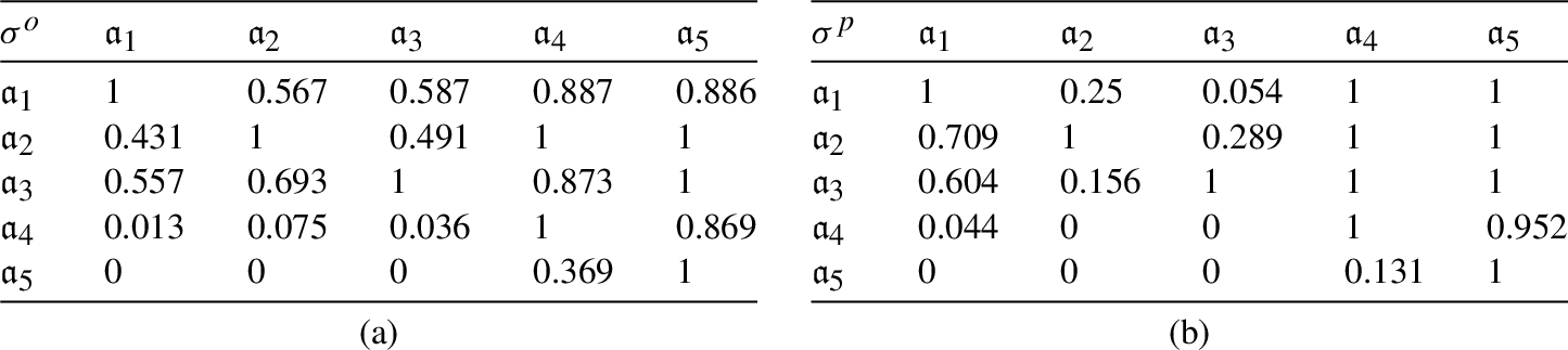
Based on the result, the first ranking is stock,
Table 13
Final ranking and score.
| Alternatives | Score | Rank |
| 1.43 | 3 | |
| 2.09 | 2 | |
| 2.22 | 1 | |
| −2.14 | 4 | |
| −3.60 | 5 |
6Sensitivity and Comparative Analyses
To check the robustness and stability of the proposed model, some sensitivity analyses, as well as a comparison analysis are carried out. These analyses are conducted to analyse various scenarios that might amend the result of the proposed model. First, a sensitivity analysis with respect to α-value is conducted for
Table 14
The score alternatives with different α.
| Degree of optimisitic attitude | |||||||||||
| 0 | 0.1 | 0.2 | 0.3 | 0.4 | 0.5 | 0.6 | 0.7 | 0.8 | 0.9 | 1 | |
| 0.95 | 1.04 | 1.14 | 1.24 | 1.34 | 1.43 | 1.53 | 1.63 | 1.72 | 1.82 | 1.92 | |
| 2.59 | 2.49 | 2.39 | 2.29 | 2.19 | 2.09 | 1.99 | 1.89 | 1.79 | 1.69 | 1.59 | |
| 2.42 | 2.38 | 2.34 | 2.40 | 2.26 | 2.22 | 2.18 | 2.14 | 2.10 | 2.06 | 2.02 | |
| −2.13 | −2.13 | −2.13 | −2.13 | −2.13 | −2.14 | −2.14 | −2.14 | −2.14 | −2.14 | −2.14 | |
| −3.82 | −3.78 | −3.73 | −3.69 | −3.65 | −3.60 | −3.56 | −3.52 | −3.47 | −3.43 | −3.39 | |
Fig. 6
Result of CIF-ELECTRE III.
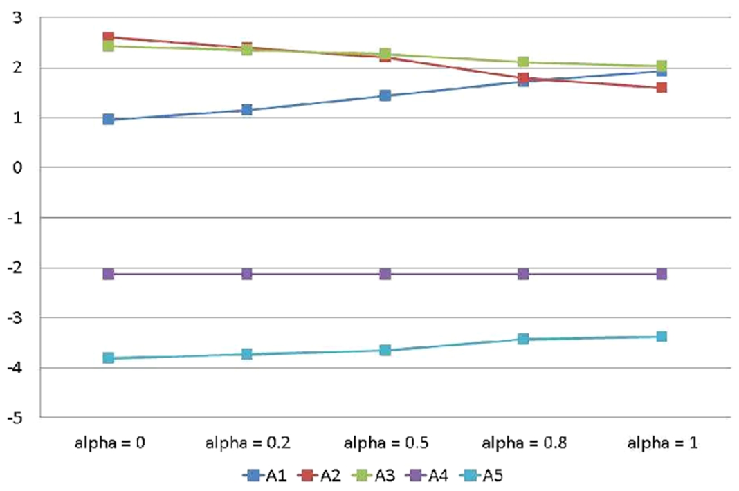
In Table 14 and Fig. 6 below, it can be noticed that the ranking for top three alternatives is slightly reversed for
Fig. 7
Sensitivity analysis of CIF-ELECTRE III based on (a) criteria weights and (b) thresholds.
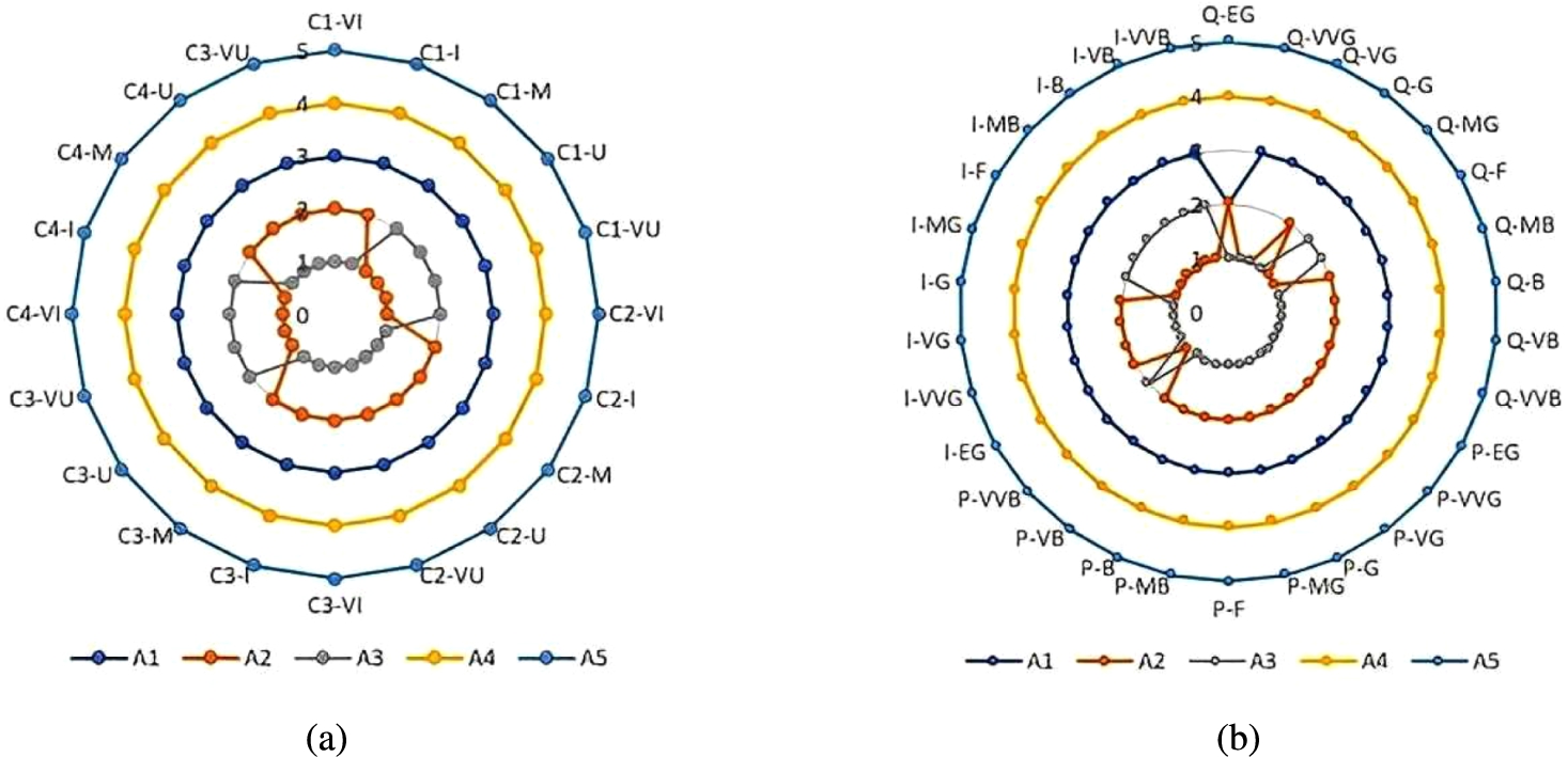
Table 15
Comparison of ELECTRE III under different sets and CIF-TOPSIS.
| Model | Information | Ranking |
| Proposed model | ||
| IF-ELECTRE III | – | |
| IVIF-ELECTRE III | – | |
| CIF-TOPSIS | ||
Furthermore, we compare the ranking results of our proposed model with ELECTRE III under two different sets: IF-ELECTRE III and IVIF-ELECTRE III (Hashemi et al., 2016). Additionally, we conduct a comparison with CIF-TOPSIS (Kahraman and Alkan, 2021).
In Table 15, it is evident that
Moreover, for a more in-depth analysis of the effect of the final decision concerning the optimistic and pessimistic attitudes, we apply the tranquillity measure proposed by Yager (1982) using the following formula:
Table 16
Tranquillity measures on CIF-TOPSIS and CIF-ELECTRE III for
| CIF-TOPSIS | 0.2649 | 0.2714 | 0.2778 | 0.2843 | 0.2907 | 0.2937 | 0.2946 | 0.2913 | 0.2879 | 0.2846 | 0.2812 |
| CIF-ELECTRE III | 0.3676 | 0.3589 | 0.3498 | 0.3417 | 0.3437 | 0.3457 | 0.3478 | 0.3500 | 0.3522 | 0.3463 | 0.3363 |
As shown in Table 16, the tranquillity measures for CIF-ELECTRE III consistently yield higher values compared to CIF-TOPSIS across all the specified α values. This demonstrates that the decisions made with CIF-ELECTRE III are associated with a better psychological ease or confidence when selecting the best alternative.
7Conclusion
In this paper, we propose an extension of the ELECTRE III model within the context of the CIFS environment for group decision analysis. We introduce several extensions to the group decision matrix (referred to as the CIF decision matrix) and the group weighting vector (referred to as the CIF weighting vector). These extensions specifically address CIFS conditions, focusing on optimistic and pessimistic attitudes. We construct these attitudinal attributes based on a set of conditional rules, ensuring that every element remains confined within a circular area defined by a radius r. We also introduce the concept of the net score degree, which serves as a unified formulation incorporating both optimistic and pessimistic scores for ranking alternatives. The net score degree is based on the parameter
However, our model has certain limitations and room for future development. Firstly, the model currently represents the attitudinal character of the entire group and does not account for individual actor attitudes. Secondly, it focuses exclusively on homogeneous group decision-making scenarios. Thirdly, in this model, CIF data is simplified to IF data for computational convenience. Future work could involve addressing individual actor attitudinal characteristics separately, accommodating heterogeneous group decision-making, and developing an algorithm that does not require converting CIF information to IF values. Lastly, it is essential to note that this study primarily deals with a simplified case involving a small group of just three experts. Discrepancies in final rankings may arise in large-scale group decision-making (LS-GDM) and more complex decision-making scenarios. Therefore, further application and analysis of our proposed method under LS-GDM are warranted.
Acknowledgements
The authors express their gratitude to the anonymous reviewers for their valuable comments and remarks that have improved the quality of the paper.
References
1 | Abdullah, L. ((2013) ). Fuzzy multi criteria decision making and its application: a brief review category. Procedia – Social and Behavioral Sciences, 97: , 131–136. |
2 | Alkan, N., Kahraman, C. ((2022) ). Circular intuitionistic fuzzy TOPSIS method: pandemic hospital location selection. Journal of Intelligent and Fuzzy System, 42: (1), 295–316. |
3 | Atanassov, K.T. ((1986) ). Intuitionisitc fuzzy sets. Fuzzy Sets and Systems, 20: (1), 87–96. |
4 | Atanassov, K.T. ((2020) ). Circular intuitionisitic fuzzy sets. Journal of Intelligent and Fuzzy Systems, 39: (5), 5981–5986. |
5 | Atanassov, K.T., Gargov, G. ((1989) ). Interval valued intuitionisitc fuzzy sets. Fuzzy Sets and System, 31: , 343–349. |
6 | Atanassov, K.T., Marinov, E. ((2021) ). Four distances for circular intuitionistic fuzzy sets. Mathematics, 9(10): , 1–8. |
7 | Atanassova, V. ((2010) ). Representation on fuzzy and intuitionistic fuzzy data by radar charts. Notes on Intuitionistic Fuzzy Sets, 16: (1), 21–26. |
8 | Beg, I., Rashid, T. ((2014) ). Group decision making using intuitionistic hesitant fuzzy sets. International Journal of Fuzzy Logic and Intelligent Systems, 14: (3), 181–187. |
9 | Boltürk, E., Kahraman, C. ((2022) ). Interval-valued and circular intuitionistic fuzzy present worth analyses. Informatica, 33: (4), 693–711. |
10 | Bozyiğit, M.C., Olgun, M., Ünver, M. (2023). Circular Pythagorean fuzzy sets and applications to multi-criteria decision making. Informatica, 1–30. https://doi.org/10.15388/23-INFOR529. |
11 | Büyükselçuk, E.Ç., Sarı, Y.C. ((2023) ). The best whey protein powder selection via VIKOR based on circular intuitionistic fuzzy sets. Symetry, 15: 1313. |
12 | Çakir, E., Taş, M.A. ((2023) ). Circular intuitionistic fuzzy decision making and its application. Expert Systems With Applications, 225: , 120076. |
13 | Chen, S.M., Tan, J.M. ((1994) ). Handling multicriteria fuzzy decision-making problems based on vague set theory. Fuzzy Sets and Systems, 67: , 163–172. |
14 | Chen, T.Y. ((2023) ). Evolved distance measures for circular intuitionistic fuzzy sets and their exploitation in the technique for order preference by similarity to ideal solutions. Artificial Intelligent Review, 56: , 7347–7401. |
15 | Chen, X., Li, J., Qian, L., Hu, X. ((2016) ). Distance anf similarity measures for intuitionistic hesitant fuzzy sets. In: International Conference on Artificial Intelligence: Technologies and Applications (ICAITA 2016). |
16 | Dubois, D. ((2011) ). The role of fuzzy sets in decision sciences: Old techniques and new directions. Fuzzy Sets and Systems, 184: (1), 3–28. |
17 | Ecer, F., Böyükaslan, A., Hashemkhani Zolfani, S. ((2022) ). Evaluation of cryptocurrencies for investment decisions in the era of Industry 4.0: a borda count-based intuitionistic fuzzy set extensions EDAS-MAIRCA-MARCOS multi-criteria methodology. Axioms, 11: (8), 404. |
18 | Forestal, R.L., Pi, S.-M. ((2022) ). A hybrid approach based on ELECTRE III-genetic algorithm and TOPSIS method for selection of optimal COVID-19 vaccines. Journal of Multi-Criteria Decision Analysis, 29: (1–2), 80–91. |
19 | Garg, H. ((2016) ). A new generalized improved score function of interval-valued intuitionistic fuzzy sets and applications in expert systems. Applied Soft Computing, 38: , 988–999. |
20 | Hashemi, S.S., Hajiagha, S.H.R., Zavadskas, E.K., Mahdiraji, H.A. ((2016) ). Multicriteria group decision making with ELECTRE III method based on interval-valued intuitionistic fuzzy information Applied Mathematical Modelling, 40: (2), 1554–1564. |
21 | Hugonnard, J., Roy, B. ((1982) ). Le plan d’extension du métro en banlieue parisienne, un cas type d’application de l’analyse multicritère. Les Cahiers Scientifiques de la Revue Transports/Scientific Papers in Transportation, 6: , 77–108. |
22 | Joshi, B.P. (2016). Interval-valued intuitionistic fuzzy sets based method for multiple criteria decision-making. International Journal of Fuzzy System Application, 5(4). https://doi.org/10.4018/IJFSA.2016100109. |
23 | Kahraman, C., Alkan, N. ((2021) ). Circular intuitionistic fuzzy TOPSIS method with vague membership functions: supplier selection application context. Notes on Intuitionistic Fuzzy Sets, 27: (1), 24–52. |
24 | Kahraman, C., Otay, I. ((2021) ). Extension of VIKOR method using circular intuitionistic fuzzy sets. International Conference on Intelligent and Fuzzy Systems, 308: , 48–57. |
25 | Kahraman, C., Öztayşi, B., Onar, S.Ç. ((2016) ). A comprehensive literature review of 50 years of fuzzy sets theory. International Journal of Computational Intelligence Systems, 9: (1), 3–24. |
26 | Khan, M.J., Kumam, W., Alreshidi, N.A. ((2022) ). Divergence measures for circular intuitionistic fuzzy sets and their applications. Engineering Applications of Artificial Intelligence, 116: , 105455. |
27 | Mohamadghasemi, A., Vencheh, A.H., Lotfi, F.H., Khalilzadeh, M. ((2020) ). An integrated group FWA-ELECTRE III approach based on interval type-2 fuzzy sets for solving the MCDM problems using limit distance mean. Complex and Intelligent Systems, 6: (2), 355–389. |
28 | Otay, I., Kahraman, C. ((2021) ). A novel circular intuitionistic fuzzy AHP and VIKOR methodology: an application to a multi-expert supplier evaluation problem. Pamukkale University Journal of Engineering Sciences, 28: (1), 194–207. |
29 | Peng, H.G., Shen, K.W., He, S.S., Zhang, H.Y., Wang, Q. J ((2019) ). Investment risk evaluation for new energy resources: an integrated decision support model based on regret theory and ELECTRE III. Energy Conversion and Management, 183: , 332–348. |
30 | Pratama, D., Yusoff, B., Abdullah, L., Kilicman, A. ((2023) ). The generalized circular intuitionistic fuzzy set and its operations. AIMS Mathematics, 8: (11), 26758–26781. |
31 | Qu, G., Qu, W., Wang, J., Zhou, H., Liu, Z. ((2018) ). Factorial-quality scalar and an extension of ELECTRE in intuitionistic fuzzy sets. International Journal of Information Technology and Decision Making, 17: (1), 183–207. |
32 | Ramya, L., Narayanamoorthy, S., Manirathinam, T., Kalaiselvan, Kang, D. ((2023) ). An extension of the hesitant Pythagorean fuzzy ELECTRE III: techniques for disposing of e-waste without any harm. Applied Nanoscience, 13: , 1939–1957. |
33 | Rouyendegh, B.D. ((2017) ). The intuitionistic fuzzy ELECTRE model. International Journal of Management Science and Engineering Management, 13: (2), 139–145. |
34 | Roy, B. ((1968) ). Classement Et Choix En Presence De Points De Vue Multiples (La Metode ELECTRE). Revue Française d’automatique, d’informatique et de Recherche Opérationnelle. Recherche Opérationnelle, 2: (8), 57–75. |
35 | Roy, B. ((1978) ). ELECTRE III: Un Algorithme de Classements Fonde Sur Une Representation Oue Des Preferences En Presence de Criteres Multiples. Cahiers Du CERO, 20: (1), 3–24. |
36 | Roy, B., Bertier, P. ((1973) ). La méthode electre II : une application au media-planning. In proceedings of the IFORS International Conference on Operational Research, pp. 291–302. |
37 | Roy, B., Vincke, P. ((1984) ). Relational systems of preference with one or more pseudo-criteria: some new concept and results. Management Science, 30(1): , 1323–1335. |
38 | Taib, C.M.I.C., Yusoff, B., Abdullah, M.L., Wahab, A.F. ((2016) ). Conflicting bifuzzy multi-attribute group decision making model with application to flood control project. Group Decision and Negotiation, 25: , 157–180. |
39 | Torra, V. ((2010) ). Hesitant fuzzy sets. International Journal of Intelligent Systems, 25: (6), 529–539. |
40 | Torra, V., Narukawa, Y. ((2009) ). On hesitant fuzzy sets and decision. In: The 18th IEEE International Conference on Fuzzy Systems, pp. 1378–1382. |
41 | Xu, C., Wen, Y. ((2023) ). New measure of circular intuitionistic fuzzy sets and its application in decision making. AIMS Mathematics, 8: (10), 24053–24074. |
42 | Xu, Z. ((2007) ). Intuitionistic fuzzy aggregation operators. IEEE Transactions on Fuzzy Systems, 15: (6), 1179–1187. |
43 | Yager, R.R. ((1982) ). Measuring tranquility and anxiety in decision making: an application of fuzzy sets. International Journal General System, 8: , 139–146. |
44 | Yusoff, B., Taib, I., Abdullah, L., Wahab, A.F. ((2011) ). A new similarity measure on intuitionistic fuzzy sets. International Journal of Mathematical and Computational Sciences, 5: (6), 819–823. |
45 | Yusoff, B., Kilicman, A., Pratama, D., Roslan, H. ((2023) ). Circular q-rung orthopair fuzzy set and its algebraic properties. Malaysian Journal of Mathematical Sciences, 17: (3), 363–378. |
46 | Zadeh, L.A. ((1965) ). Fuzzy sets. Information And Control, 8: , 338–353. |
47 | Zadeh, L.A. ((1975) ). The concept of a linguistic variable and its application to approximate reasoning—I. Information Sciences, 8: (3), 199–249. |
48 | Zhao, T., Xiao, J. ((2012) ). Type-2 intuitionistic fuzzy sets. Control Theory and Application, 29: , 1215–1222. |


