
An Effective Solution for Drug Discovery Based on the Tangram Meta-Heuristic and Compound Filtering
Abstract
Ligand-Based Virtual Screening accelerates and cheapens the design of new drugs. However, it needs efficient optimizers because of the size of compound databases. This work proposes a new method called Tangram CW. The proposal also encloses a knowledge-based filter of compounds. Tangram CW achieves comparable results to the state-of-the-art tools OptiPharm and 2L-GO-Pharm using about a tenth of their computational budget without filtering. Activating it discards more than two thirds of the database while keeping the desired compounds. Thus, it is possible to consider molecular flexibility despite increasing the options. The implemented software package is public.
1Introduction
1.1Overview
The drug discovery process is a major challenge in the real-world scenario of today, where different factors play a role (Hughes et al., 2011). This implies that developing new drugs costs, on average, more than 1 billion USD and can take between 12 and 15 years at all stages (Sumudu and Leelananda, 2016; Ban et al., 2017). To speed up this process and reduce costs, there is a continuous process of designing and implementing new techniques from traditional medicine (Fu et al., 2017) to High Throughput Screening (HTS) infrastructures (Zeng et al., 2020).
In this context, Virtual Screening (VS) is a relevant in silico technique in drug discovery that can help identify potential drug candidates with high efficacy and safety profiles (McInnes, 2007). In fact, VS has helped bring to market compounds such as ritonavir, nelfinavir, saquinavir (Kanhed et al., 2021) or plasmepsin inhibitors (Meissner et al., 2019). There are two types of VS methods depending on the information obtained from compounds: Structure-Based VS (SBVS) and Ligand-Based VS (LBVS). SBVS methods (Maia et al., 2020) require knowledge of the structure of the target protein, which to obtain involves a set of challenges (Parois et al., 2015). Consequently, in most cases LBVS are the only methods that can be applied because they do not require knowledge of the 3D structure of the target molecule (Hamza et al., 2012).
LBVS methods are used to identify molecules in a database similar to another reference compound. To do so, they compare the structural and physicochemical properties (descriptors) of the reference molecule with those of compounds in the database, which may contain millions of compounds. Considering the latter, the computational efficiency of mathematical models that describe molecular descriptors is crucial. Despite the relatively low cost per evaluation, evaluating descriptors for thousands for a molecule, and subsequently for millions of molecules, can quickly become unaffordable in terms of time. Therefore, there is a need to prioritize descriptors that are computationally efficient to enable efficient screening of large numbers of molecules. Shape similarity has been identified as a descriptor of choice due to its ability to detect potential drug candidates that may have different chemical structures but similar shapes, which may mean that they exhibit similar biological activities (Carracedo-Reboredo et al., 2021; Kumar and Zhang, 2018), as well as its low computational cost. Consequently, shape similarity will be the descriptor used in this work to compare the quality of the different algorithms.
Finally, the flexibility of the molecules has to be also taken into account in LBVS problems (Rapaport, 2004). Although literature works have mainly considered molecules as rigid objects, the reality is that molecules vary their interatomic distances and angles between atoms, giving rise to conformations, i.e. the same molecule with different interatomic distances and they potentially have different behaviours with other compounds and proteins. Consequently, flexibility must be taken into account when applying LBVS as it allows solutions to be found that would otherwise not be possible. The simplest example would be to find two identical molecules with different conformations: if conformations are not explored, no matter how good the search algorithm is, it will never find such a compound, or at least not with the desired percentage of similarity. On this basis, everything looks good for flexibility. However, the reason why it is not considered is that it increases computational calculations enormously as hundreds of different conformations can be generated from each molecule. To deal with this, filters are often applied to discard compounds before generating the conformations in order to avoid a large number of comparisons that would not return a promising result (Ellingson et al., 2014; Poongavanam et al., 2021). However, this is influenced by the quality of the filter, as compounds that a priori do not seem to be good candidates can be discarded. In this work, we are going to use the software OMEGA (Hawkins et al., 2010) for the generation of conformations because of its widespread use in the literature and to facilitate future comparisons. Regarding the filters to discard compounds, we have included our own system, to be used as desired, in order not to consume too many computational resources.
1.2Related Works
Identifying compounds with similar shapes is a computationally demanding problem due to two main reasons: First, there is a vast number of molecules to analyse, up to millions. Secondly, finding the position of maximum overlap between every pair of molecules for the comparison to be descriptive is hard. Consequently, an exhaustive search is not feasible, and local search methods are frequent (Wang et al., 2020; Ahmed et al., 2018). Similarly, heuristics and meta-heuristics are often employed to achieve satisfactory solutions with reasonable computational effort (Lindfield and Penny, 2017; Salhi, 2017).
One of the most recent proposals among population-based meta-heuristics is OptiPharm (Puertas-Martín et al., 2019; Puertas-Martín et al., 2022). It offered several advantages over the state-of-art 3D alignment optimization methods ROCS (Software et al., 2008) and WEGA (Yan et al., 2013). Specifically, it outperformed them in the quality of solutions and execution time while also being highly configurable. An even more recent population-based algorithm is 2L-Go-Pharm (Ferrández et al., 2022). It improved the quality of the OptiPharm solutions and reduced the number of function evaluations required. These methods were designed to be able to explore the entire search space both broadly and deeply, thus avoiding being confined to a local minimum. This feature is particularly useful for complex molecules with numerous degrees of freedom, as it allows for a comprehensive exploration of the search space.
Both OptiPharm and 2L-Go-Pharm are population-based algorithms that apply different techniques to a population to explore the optimal solution. OptiPharm uses the concept of species associated with a radius that decreases as the iterations progress (Jelasity et al., 2001). In contrast, 2L-Go-Pharm uses a 2-level design in which the first one tries to detect solutions that have the potential to be local or global optima, and in the second level, these solutions are guided to the peaks. As population-based methods, they have high exploration capabilities (Lindfield and Penny, 2017; Salhi, 2017) and are intrinsically compatible with parallel computing (Boussaïd et al., 2013; Sudholt, 2015; Storn and Price, 1997). On the other hand, they generally have multiple parameters to tune that significantly affect the search performance (Jones and Martins, 2021; Rao et al., 2012). Besides, they generally need numerous objective function evaluations to ensure remarkable and stable results (Costa and Nannicini, 2018; Cruz et al., 2022a). Accordingly, OptiPharm expects four parameters, and its robust configurations start from computational budgets of 200 000 (2L-Go-Pharm, 150 000) objective function evaluations (Puertas-Martín et al., 2019), yet it can benefit from parallel computing (García et al., 2023) as an evolutionary method.
1.3Contributions
The main contribution of this work is presenting the optimization algorithm Tangram CW. It is especially suitable for addressing shape similarity-based LBVS problems with rigid and flexible molecules. Nevertheless, the method is decoupled from the objective function and does not compute derivatives. Hence, it can be studied for different objective functions (problems) and can be classified as a black-box derivative-free optimizer (Costa and Nannicini, 2018). The algorithm is a new version of the proposal made by the authors in (Cruz et al., 2022b) and that showed promising results with a reduced consumption of function evaluations. The changes, which make the algorithm very effective for the problem at hand, are related to the division of the search space and the definition of variables that wrap around their bounds. It only expects two parameters: the total number of function evaluations and those consumed by the local search component every time. They can be directly related to the exploration and exploitation facets of search methods (Jones and Martins, 2021; Van Geit et al., 2008), i.e. reaching new regions of the search space and obtaining the best point out of the known ones, respectively.
Another relevant contribution of this work is a knowledge-based filter of compounds. Other algorithms, such as OptiPharm, rely on pre-defined position vectors representing promising solutions. They mainly improve the quality of the solutions obtained but do not allow discarding any compound in advance. In other words, although every compound in the considered database will be compared to the query or reference one in these descriptive positions, most will differ significantly from the beginning. Accordingly, this work defines an optional component that ranks every compound at these positions and discards those exhibiting low values considering a user-given tolerance. This aspect can be critical when working with flexibility, as databases increase so much in size that explorations graze infeasibility despite parallel computing. This tool is separated from the proposed optimizer and can be used independently.
Finally, the problem-level parallelization, i.e. how compounds are accessed, is considered from the beginning of the design of the proposed solution. Again, it is independent of the optimizer and the compound filter. Focusing on this side simplifies the management of parallel hardware, ensures relevant workloads, and is independent of the parallelization capabilities of the chosen optimizer. The implemented software package is publicly available in Cruz et al. (2023).
The rest of the paper is structured as follows: Section 2 explains the proposed methodology from the compound positioning model and the objective function to the parallel database exploration workflow, the compound filter, and the designed optimizer. Section 3 describes the experimentation carried out to assess the proposal. Finally, Section 4 draws conclusions and proposes future work.
2Materials and Methods
This section describes the application framework of LBVS using the shape similarity metric and the proposed solution. Firstly, we define the Gaussian-model used to evaluate the similarity between two molecules. After that, the section describes the parallel exploration of compound databases for rigid and flexible molecules, the optional knowledge-based filter, and the proposed optimizer.
2.1Positioning Model
As introduced, comparing two molecules requires applying a rotation and translation to one of them. In this work, such modification is defined by 10 variables in total. The first 7 define the rotation and the last 3 the translation. The first group of parameters can be divided into three sub-groups, the first parameter defines the rotation that is applied on the axis generated by the two 3D points generated with the following six parameters. Finally, the translation uses 3 parameters to be able to move the molecule on any axis.
These parameters are constrained to speed up the process and to avoid generating positions where there is no overlap. The rotation parameter is contained in the range
2.2Shape Similarity Metric
The shape similarity between two compounds is calculated by obtaining the overlap between their atoms using the Gaussian-model. This model is widely used in the literature for its trade-off between solution quality and performance, and it takes the concept of the Gaussian function and assimilates it to the density distribution function of an atom. It is used by other popular software such as ROCS (Software et al., 2008), WEGA (Yan et al., 2013), OptiPharm (Puertas-Martín et al., 2019) and 2L-GO-Pharm (Ferrández et al., 2022) in different versions.
To obtain the shape similarity between an A and a B molecule, we use the model defined in Yan et al. (2013) which incorporates a weight associated with each atom, thus improving the model. The similarity value is given by the following expression:
(1)
(2)
(3)
Note that the maximum value of the function in (1) depends on the number of atoms of the analysed molecules. Consequently, these values must be normalized to compare the results. For this, a standard in the literature is to use the Tanimoto similarity (Cereto-Massagué et al., 2015; Rogers and Tanimoto, 1960), which returns a value in the range
(4)
2.3Database Exploration Procedure
2.3.1Standard LBVS Search Process
In this context, one can define a search for similar compounds from the reference or query compound and the database to scan. Algorithm 1 describes the main steps of a basic LBVS seek process. Its fundamental parameters are the information of the reference compound (query) and the database to explore (database). In practical terms, the database refers to a directory containing a file with the details of every compound. Their identification depends on their file name. For example, one of the files in the dataset later used at experimentation is ‘DB00014.mol2’. The third parameter defines the comparison criterion, i.e. the Tanimoto similarity (
The procedure starts with loading the information of the query compound at line 1, i.e. a matrix with the details of every atom (matQ). This is used to compute the weighting (wQ) and overlap (ovQ) factors at lines 2 and 3, respectively. As the query is fixed, there is no need to repeat the specific computations, which can be obtained once and stored. After that, at line 4, the query is sought and excluded from the database. Otherwise, any robust search will always return the query itself as its most similar compound. However, readers should note that omitting the self-exclusion allows testing the robustness of proposals, as they should find the same compound sought. The preliminary stage ends by initializing the ordered list that will contain the most similar compounds found.
Algorithm 1
Standard process for exploring a compound database:
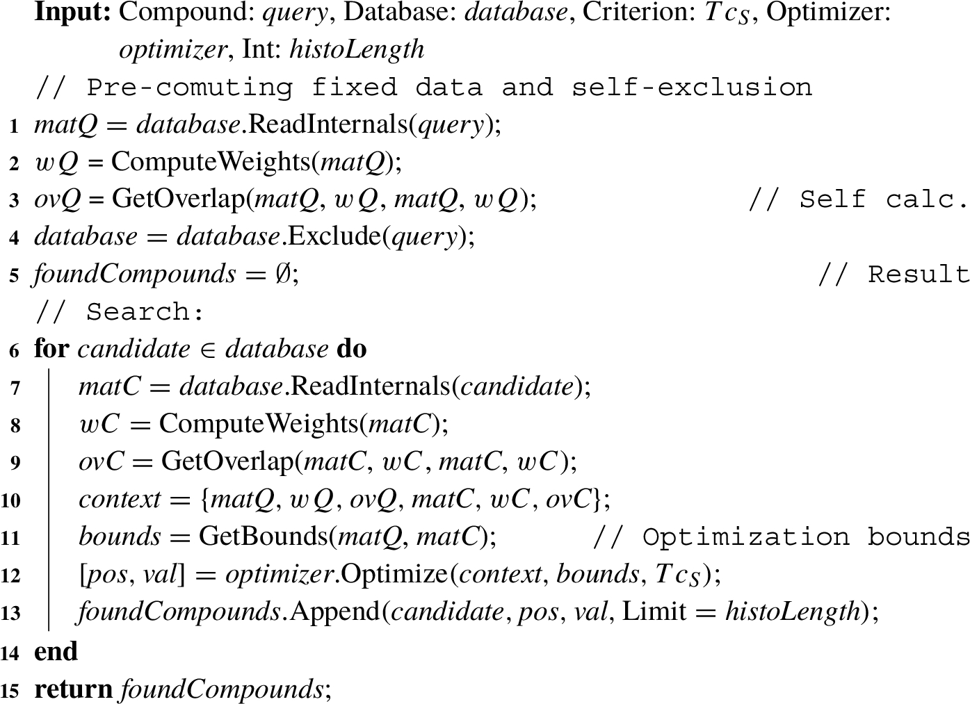
The search, which is defined between the lines 6 and 14, repeats the same process for every compound in the database. Specifically, it loads the matrix with the information of the atoms defining the current candidate (matC), which lets us compute its specific weighting (
The critical and most computationally demanding part of every iteration of the search is at line 12. It launches the chosen optimizer to find the best comparison position of the candidate compound. This procedure will always try to find the position (pos) that results in the highest value (val), i.e. the Tanimoto similarity,
2.3.2Parallelization Strategy
The search process described in Algorithm 1 is mainly embarrassingly parallel (Trobec et al., 2018). More specifically, the initialization stage is common and fixed. The search ultimately becomes a loop that takes every compound in the database and places it as well as possible using the optimizer. Positioning a compound, which is the most computationally demanding part, does not depend on the others. Hence, a parallel implementation of this search only needs to split the iterations of the loop into concurrent execution units.
Achieving this kind of parallelization is straightforward using tools offering high level of abstraction, such as the ‘parallel for’ construction of the OpenMP API (Trobec et al., 2018) and the ‘parfor’ loop of MATLAB (Cruz et al., 2022a). The former also allows adjusting the scheduling to minimize load unbalancing and idle execution units, as the iterations involving candidate compounds with numerous atoms take longer. Regardless, this aspect could be neglected assuming a uniform distribution of compound sizes in the database.
However, there is a critical point to consider for a proper parallel implementation in a shared-memory environment: The
Another option is to define a local version of
2.3.3Modifications to Support Flexibility
As mentioned, Algorithm 1 expects a database with a single file for every different compound. That situation occurs when working with rigid molecules, but it is incompatible with considering flexible molecules. Since they have bonds that can rotate, covering different positions involves generating multiple files per compound by rotating their flexible bonds by different angles. They are generated in advance, as a preliminary stage. Intuitively, it can be compared to storing multiple pictures of a person from different angles to find better coincidences with other people. This process, known as generating the conformations of molecules (Puertas-Martín et al., 2022), is expected to improve the results of LBVS by avoiding overlooking some compounds in favour of others. However, it also results in multiple data files per compound. Fortunately, adapting the standard exploration procedure to support this situation is straightforward in practical terms.
Specifically, the previous example file ‘DB00014.mol2’ will now be translated into multiple files with the following naming structure: ‘DB00014_conf1. mol2’, ‘DB00014_conf2.mol2’, and so on, depending on the number of conformations. Rigid compounds will still have a single representing file, but flexible ones might result in a few tens or even hundreds. In this context, the modifications of Algorithm 1 start with postponing lines 1 to 3, as there might not be a single reference to fix. It is also necessary to modify (generalize) the self-exclusion process at line 4. Instead, it should now scan the files defining the database and produce two lists: one with the compounds to compare the query with (
Regarding the
After the previous modifications, the search part is modified to start with an external loop that simply changes the query conformation, i.e. for
Notice that the parallelization strategy can be directly imported to the inner loop, i.e. in the per-query search, as in the standard approach. It ensures a significant amount of work for every execution unit. Moreover, although some compounds may have hundreds of conformations, others may have tens or even just one. Hence, dividing the space of potential compounds seems a more sensible and scalable option.
2.4Compound Filter
Either the standard search process or the one dealing with conformations, comparing the query compound to the rest of the database is computationally demanding. The reason is the effort made to find the most descriptive relative position between the query and every candidate, i.e. solving multiple optimization problems. However, although every optimizer will try to find the best position in every case, most will be useless in the end. For example, let us consider a database with 2 001 rigid compounds and a computational budget of 200 000 objective function evaluations per comparison (positioning). Executing Algorithm 1 for a particular query will take
In this context, it would be useful to discard (ignore from the database) those compounds having very low probabilities of matching the query. In terms of Chemistry, it could be possible to define a preliminary filter considering, for instance, the number of atoms defining the compound. However, generic criteria may significantly diverge from the particular magnitude of interest (e.g., Tanimoto’s shape similarity). It also implies studying other aspects. For this reason, this work proposes to use the same objective function to identify those compounds whose preliminary assessments are so different from the best ones that it seems logical to ignore them.
Unfortunately, computing the objective function involves defining a relative position between the query and candidate compound, i.e. relying on an initial solution for the corresponding optimization problem. However, it would not make sense to solve the positioning problem in order to avoid doing so. Besides, some of the global optimization methods used for the target problem, such as OptiPharm and the proposed Tangram algorithm, are not deterministic. Hence, using them to discard options doubles the uncertainty, and their choice would be virtually random without investing a significant amount of objective function evaluations. Aside from these inconveniences, stacking complete optimizers make tuning the search harder. Therefore, the proposal of this work is to preliminary rank compounds after considering a very reduced set of descriptive pre-defined positions.
Specifically, the proposed filter maintains the scheme of Algorithm 1 with two main modifications. The first is replacing the call to an external optimizer by directly studying four pre-defined solutions, i.e. positioning vectors, for the query and every candidate (potentially filtered) compound. At this point, the value of every compound is kept, so the previous ‘Append’ function limiting the records to
The second and last change represents the real filtering procedure. More specifically, after having preliminary explored the database and recorded the maximum value for every compound at one of the four initial positions, it is necessary to select a subset of them. The proposed filter offers two options for this purpose depending on a single parameter,
The described procedure should be launched to explore and reduce the size of the input database after removing the query or reference compound and before starting the complete (optimization-based) search, e.g. between lines 4 and 5 of Algorithm 1. This filter will only execute four objective function evaluations per compound, and can be executed in parallel, too. This process is also compatible with parallel computing. Similar to Algorithm 1, the most direct approach is to parallelize the loop focused on assessing every compound, i.e. computing independent the preliminary values and storing them at the corresponding indices.
2.5Tangram CW
2.5.1Background
The Tangram algorithm presented in Cruz et al. (2022b) is a black-box minimization meta-heuristic defining a reduced set of exploration rules, using (but not linked to) the SASS stochastic hill-climber for local optimization. Tangram, which expects two parameters at most, requires a normalized search space in which every search or decision variable is in the range
(5)
In this context, Tangram starts by evaluating the centre of the hypercube, which becomes the current result. The method also decides to launch its standard mode or its incisive one. The former consists of three consecutive stages, global, division, and local, in a loop that ends after consuming all the evaluations. The global stage launches the local search from the current result and makes the maximum step size to cover the whole search space, which changes the current solution to a new one every time a better candidate solution is found. The division stage computes and evaluates the midpoint between the current solution and each corner of the search space. After that, the local stage launches the local search from these midpoints, starting with the best ranked, just in case the evaluation budget runs out before the stage ends. The main loop body ends by replacing the current solution with the best point reached during the local phase if any of them outperforms it. The incisive mode is mainly the same but merges the division and local stages. More specifically, it launches the local search from every midpoint immediately after having computed it, which makes it impossible to prioritize them but ensures local-sharpened results when the total evaluation budget is relatively low. For this reason, the incisive mode is only activated when the total number of function evaluations is lower than the number of corners, i.e.
The results achieved by Tangram with the benchmarks proposed in Costa and Nannicini (2018) for very low computational budgets were competitive. Considering them, along with the common roots and local search component, Tangram was also used to replicate the results of OptiPharm in Puertas-Martín et al. (2019) at shape similarity LBVS. However, these preliminary results were not competitive, and there was room for improvement.
As the objective function is fast to compute, the number of allowed evaluations can be significantly greater than expected when designing the original method. Despite this possible increase in the computational budget, the problem dimensionality results in
Hence, the proposed version of Tangram will launch the local search from the centroid of every region defined by the current best solution and its nearest corners. There will be
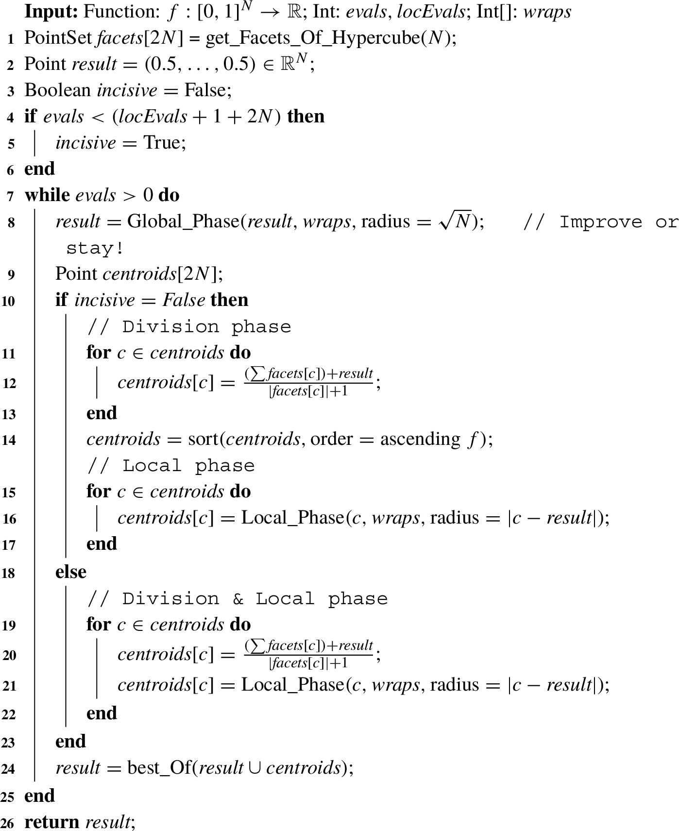
2.5.2Workflow of Tangram CW
Tangram CW, which inherits the background from its ancestor, follows Algorithm 2. The underlying process remains the same as outlined in the previous section for the original Tangram. Thus, the algorithm takes the centre of the search space as the initial solution to alternating a global stage with either i) a division and a local search phase (standard mode) or ii) a combination of both (incisive mode). For conciseness, let us focus on the differences with the original algorithm.
Algorithm 2
Tangram CW
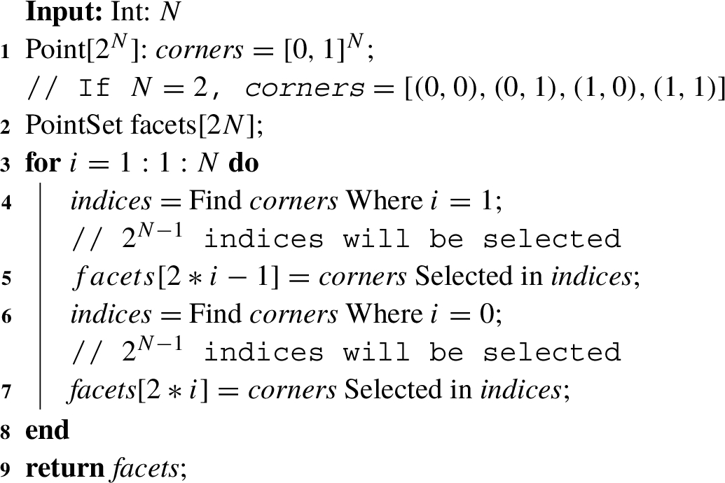
Algorithm 3
get_Facets_Of_Hypercube
Firstly, the number of function evaluations that every local search takes is explicitly considered a parameter to tune, i.e.
Secondly, at line 1, the statement
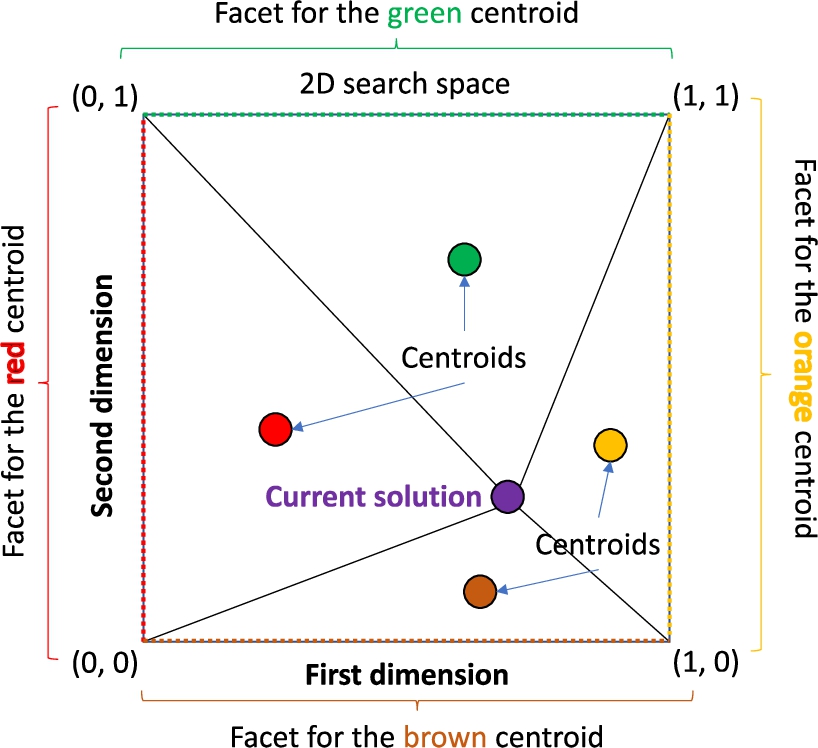
Fig. 1
Set of facets for computing the division centroids when
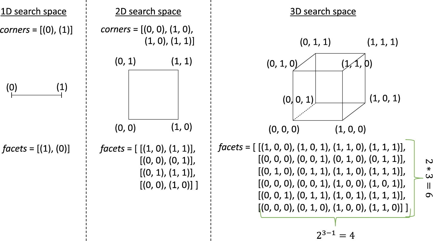
Fig. 2
Corners used for computing each centroid in a 2D search space (Division stage).
Thirdly, the mode selection from lines 3 to 6 in Algorithm 2 is conceptually equivalent to that in the original method. However, it takes into account that the new algorithm takes
Fourthly and lastly, the global stage at line 8 keeps the maximum step (radius) of the local search component to the diameter of the search space, as in the original Tangram algorithm. However, this radius is set to the distance between the centroid of every region and the current solution at local phases (lines 16 and 21). Conversely, the original Tangram method would have set this value to the distance from the current solution and the midpoint between it and the corner involved. Independent of the alias ‘global’ or ‘local’, the calls at lines 8, 16, and 21 in Algorithm 2 refer to the local search component, SASS. This method is not described due to space limitations, but the interested reader can find detailed explanation in Lančinskas et al. (2013), Cruz et al. (2022b). That said, bound checking must be modified to make the variables indexed in
2.5.3Final Remarks
The previous explanation of Tangram CW is mainly problem-independent. Adapting the problem-specific objective function defined in (4) is straightforward. It is only necessary to normalize the ten input variables so that the function domain becomes the 10-dimensional unit hypercube. However, as that function returns the overlap degree between the query and the studied compound, the optimizer should try to maximize it. Tangram CW, like the original method (and most optimization algorithms) is described in terms of minimization. Fortunately, converting a maximization problem into a minimization one is trivial. It is only necessary to multiply the objective function by −1, i.e. maximizing f is equal to minimizing
It is also relevant to highlight that the incisive mode of Tangram CW is not likely to be used for this problem. However, it is defined for generality, as it addresses a potentially unwanted situation like the original method. Other applications of Tangram CW in which very few function evaluations are allowed could benefit from it.
3Experimentation and Results
This section starts by explaining the implementation of the proposed solution. The description covers both software and hardware. After that, it presents the dataset used for the different experiments. Specifically, the experimentation initially compares the performance of the proposed optimizer, Tangram CW, to the state-of-the-art global methods for shape similarity-based screening OptiPharm and 2L-Go-Pharm. The comparison replicates the benchmarks defined by those methods for rigid compounds and focuses on reducing the computational budget. In this context, the second experimentation stage studies the effectiveness of the proposed filtering strategy to discard unwanted compounds while keeping the expected ones. The third and last experimentation phase analyses the effectiveness of the proposed optimizer and compound filter when considering the flexibility of the compounds in the dataset, which defines the most challenging situation. Aside from describing how the proposal performs, the study also discusses the general benefits of considering flexibility despite the practical difficulties, as it is only possible when relying on highly efficient methods.
3.1Implementation and Hardware Setup
The proposed solution has been implemented in MATLAB (2018) and C through the MEX API to accelerate the most computationally demanding parts (Getreuer, 2010; The MathWorks Inc., 2022). Specifically, the parallel database exploration processes, the compound filter, and the optimizer are written in MATLAB. Conversely, those linked to the objective function calculation are written in C and compiled as MATLAB Executable files through the MEX API. This way, the overall procedure is wrapped into the MATLAB environment. As a high-level-of-abstraction language, its use results in concise and maintainable code that allows modifications easily, especially considering the numerous toolboxes developed for MATLAB (Cruz et al., 2022a). At the same time, the most computationally intensive part remains written in C and compiled for the architecture to run more efficiently. To become conscious of the effectiveness of this approach, at preliminary experimentation, the same virtual screening process was accelerated by 4.11 times after replacing the initial MATLAB version of the objective function with the C-MEX one in the development workstation. The implemented software package is publicly available in Cruz et al. (2023).
Regarding the hardware used, the development workstation features an Intel Core i7 processor with 4 physical cores and 32 GB of RAM running Xubuntu 18.04. Aside from development purposes, this machine has also been used for the experiments with rigid compounds. However, for the virtual screening processes dealing with flexible compounds through the generation of multiple conformations, a node of the cluster of the Supercomputing – Algorithms research group from the University of Almería, Spain, is used. It has 2 AMD EPYC Rome 7 642 with 48 cores each (96 in total) and 512 GB of RAM.
3.2Food and Drug Administration (FDA) Database
The Food and Drug Administration (FDA) (Ciociola et al., 2014) is a federal agency of the United States Department of Health and Human Services. It is responsible for safeguarding and improving public health through the regulation of prescription and over-the-counter medications. Among the resources that they offer publicly, there is a dataset containing 1 751 molecules representing safe and approved drugs for use in humans in the USA. In the current context, it is customary to identify compound pairs in the FDA database that exhibit a high level of similarity. The background to this is that finding new compounds can be a valuable approach to drug discovery, as it can potentially lead to a more effective, safer, and more efficient development of new treatments (Wishart, 2006).
Additionally, the selection of these compounds was used to test the software with flexible compounds. For this purpose, the software OMEGA (Hawkins et al., 2010) was used with the default configuration and the maximum number of conformations was set at 500. Consequently, a novel database of 279 756 conformations was generated from the original 1751 through this process.
3.3Battery of Searches for Rigid Compounds
The performance of the proposal has been first studied by replicating one of the most descriptive tests considered when introducing OptiPharm and 2L-GO-Pharm. Namely, the benchmark consists of 40 query molecules from the FDA database, without flexibility, and considering hydrogen atoms. The latter aspect is highly relevant because some state-of-the-art tools, such as WEGA, omit hydrogen atoms during the search to accelerate the process, yet it may affect results. Nevertheless, OptiPharm achieved competitive results considering them. The optimizer used its robust configuration, which provides the method with a computational budget of 200 000 (200k) objective function evaluations for every positioning procedure. The reader can find more details about these results in Puertas-Martín et al. (2019) (Table 5). Later, 2L-GO-Pharm obtained comparable results after reducing the computational budget to 150k (Ferrández et al., 2022). They define the ground truth for the proposal, i.e. Tangram CW with and without compound filtering (and supported by parallel computing at both levels).
The local search method, SASS, uses its default configuration as suggested in Cruz et al. (2022b) and also done by OptiPharm. The configuration of Tangram CW was adjusted after preliminary experimentation letting it use from 5 to 20k objective function evaluations and local budgets ranging from 32 to 256. The first problem dimension, i.e. the only angular rotation, was finally set to wrap around at bounds. The selected configuration defines 20k function evaluations, and every local search takes 128. Hence, Tangram CW will work with 10% and 13.33% of the computational budgets of OptiPharm and 2L-GO-Pharm, respectively.
Table 1
Results of Tangram CW (20k evaluations) compared to OptiPharm (200k evaluations) and 2L-GO-Pharm (150k evaluations) when searching for 40 rigid compounds.
| OptiPharm/2L-GO-Pharm | Tangram CW | |||||
| ID | Query | Atoms | Found C. | Value | Found C. | Value |
| 1 | DB00529 | 10 | DB09294 | 0.87 | DB09147 | 0.87 |
| 2 | DB00331 | 20 | DB09210 | 0.86 | DB09210 | 0.86 |
| 3 | DB01352 | 29 | DB00306 | 0.89 | DB00306 | 0.89 |
| 4 | DB01365 | 30 | DB00191 | 0.94 | DB00191 | 0.93 |
| 5 | DB00380 | 35 | DB01041 | 0.85 | DB01041 | 0.85 |
| 6 | DB06216 | 37 | DB00370 | 0.88 | DB00370 | 0.88 |
| 7 | DB00693 | 37 | DB01619 | 0.86 | DB01619 | 0.86 |
| 8 | DB07615 | 40 | DB00721 | 0.79 | DB00721 | 0.79 |
| 9 | DB09219 | 40 | DB01320 | 0.85 | DB01320 | 0.85 |
| 10 | DB00674 | 42 | DB01619 | 0.80 | DB01619 | 0.80 |
| 11 | DB01198 | 45 | DB00402 | 0.89 | DB00402 | 0.89 |
| 12 | DB00887 | 45 | DB00837 | 0.74 | DB00837 | 0.74 |
| 13 | DB00246 | 50 | DB01261 | 0.76 | DB01261 | 0.75 |
| 14 | DB00381 | 53 | DB01023 | 0.83 | DB01023 | 0.83 |
| 15 | DB09237 | 54 | DB01054 | 0.75 | DB01054 | 0.75 |
| 16 | DB00876 | 54 | DB09039 | 0.67 | DB09039 | 0.67 |
| 17 | DB00254 | 55 | DB00595 | 0.85 | DB00595 | 0.85 |
| 18 | DB00351 | 57 | DB04839 | 0.93 | DB04839 | 0.93 |
| 19 | DB01196 | 60 | DB00286 | 0.80 | DB00286 | 0.80 |
| 20 | DB01621 | 66 | DB01148 | 0.72 | DB01148 | 0.71 |
| 21 | DB09236 | 66 | DB01054 | 0.68 | DB01054 | 0.68 |
| 22 | DB08903 | 69 | DB00333 | 0.68 | DB00333 | 0.68 |
| 23 | DB00632 | 69 | DB00464 | 0.74 | DB00464 | 0.74 |
| 24 | DB01419 | 70 | DB06605 | 0.67 | DB06605 | 0.67 |
| 25 | DB00320 | 80 | DB00728 | 0.62 | DB00728 | 0.62 |
| 26 | DB00728 | 91 | DB01339 | 0.84 | DB01339 | 0.84 |
| 27 | DB00503 | 98 | DB00701 | 0.54 | DB01336 | 0.54 |
| 28 | DB01232 | 100 | DB00212 | 0.62 | DB00212 | 0.62 |
| 29 | DB00309 | 110 | DB00541 | 0.62 | DB00541 | 0.62 |
| 30 | DB04786 | 120 | DB00511 | 0.43 | DB00511 | 0.43 |
| 31 | DB09114 | 130 | ∗DB08993∗ | ∗0.51∗ | DB01321 | 0.52 |
| 32 | DB06439 | 137 | DB00207 | 0.59 | DB00207 | 0.59 |
| 33 | DB01078 | 140 | DB00511 | 0.58 | DB00390 | 0.58 |
| 34 | DB01590 | 151 | DB00877 | 0.56 | DB00877 | 0.56 |
| 35 | DB04894 | 152 | DB00646 | 0.54 | DB00646 | 0.54 |
| 36 | DB00403 | 167 | DB08874 | 0.47 | DB08874 | 0.47 |
| 37 | DB00732 | 169 | DB06287 | 0.48 | DB06287 | 0.48 |
| 38 | DB00050 | 194 | DB00569 | 0.49 | DB00569 | 0.49 |
| 39 | DB06699 | 221 | DB09099 | 0.51 | DB09099 | 0.51 |
| 40 | DB06219 | 229 | DB00512 | 0.44 | DB06287 | 0.44 |
| Mean: | – | 86 | – | 0.70 | – | 0.70 |
Table 1 contains the results achieved for the described test. The first column has the number of every test for easier referring. The second column shows the name of the query of the reference molecule. The third one includes its number of atoms (considering those of hydrogen). The fourth column displays the most similar compound found by OptiPharm and 2L-GO-Pharm for every case. It is followed by the approximated value of the objective function that they found in the fifth column. This representation assumes that OptiPharm and 2L-GO-Pharm behave equally to save room, and that is true in 39 of the 40 cases. However, the result that the latter finds for the thirty-first case is the same as our proposal in reality. The asterisks warn the reader about this detail. Analogously, the sixth and seventh columns show the most similar compound suggested by Tangram CW and its value in the position achieved at optimization, respectively. The last row includes the average of the number of atoms and the value of the results found by the reference optimizers and Tangram CW in the corresponding columns. The values in bold font highlight either a relative victory of a method over the other or an interesting situation, and they are commented below.
For the sake of completeness, notice that it took approximately 9 hours to complete the test in the workstation, running in parallel in four cores and without compound filtering. Regardless, as run times are machine-dependent, the focus will stay on function evaluations.
At first glance, the reference optimizers and Tangram CW find the same results in most cases, covering both the suggested compound and the assessment. In five cases, i.e. 1, 27, 31 (related to OptiPharm only), 33, and 40, Tangram CW suggested different yet equally-ranked compounds. This situation, promoted when changing the methods, is interesting as it might catch the attention of analysts over new compounds for later stages of experimentation. Regardless, as mentioned, most records in Table 1 are the same on either side. There are only four numerical variations in bold (4, 13, 20 (left), and 31 (right)), and they are negligible in this context, with the resulting averages also being equal. Accordingly, both sides are equivalent in practical terms.
Nevertheless, it is necessary to remember that the computational budget of Tangram CW is approximately a tenth of that of the reference methods. More specifically, our optimizer completes the benchmark after consuming
Therefore, as intended, the results confirm that the proposed optimizer is significantly more efficient than the previous global optimization approaches for shape similarity-based screening, i.e. OptiPharm and 2L-GO-Pharm. This aspect is critical when the databases increase in size, as when considering flexibility. Aside from that, our optimizer is also simpler to implement and tune.
3.4Preliminary Compound Filtering
The aforementioned consumption of function evaluations for the benchmark of rigid compounds has two variable terms, the computational budget per positioning case and the number of compounds in the database. Tangram CW has already made it possible to change the former from either 200k or 150k to 20k only. However, the proposed compound filter can also help us to reduce the latter by minimizing the number of compounds that pass to a complete optimization-based positioning process. Some readers might consider 1 751 low enough, but it is only a benchmark. Other databases can increase the number of options significantly. Besides, the chosen benchmark will increase in size from 1 751 to 279 756 after considering flexibility through the generation of conformations, as covered in the next section. Therefore, it is highly relevant to be able to reduce the number of compounds to consider during the virtual screening process.
In this context, the knowledge-based filtering strategy has been tested for the previous benchmark in its two main configurations. Specifically, the filter has been launched to reduce the number of rigid compounds from the FDA database i) considering a degradation threshold with respect to the best ranked and ii) directly selecting a user-given number of the best. Table 2 contains the results obtained. The first three columns refer to fixed selections, i.e. the filtering parameter
Table 2
Effect of compound filtering over the rigid dataset.
| Success rate | 75% | 85% | 92.5% | 82.5% | 92.5% | 100% |
| (30/40) | (34/40) | (37/40) | (33/40) | (37/40) | (40/40) | |
| Ave. no. of compounds left | 100 | 250 | 500 | 205 | 348 | 522 |
| (5.71%) | (14.28%) | (28.56%) | (11.71%) | (19.87%) | (29.81%) |
It is possible to achieve high success rates despite discarding multiple compounds before optimization. Even if one keeps the 100 most promising compounds, i.e. the results of the first column, the expected compound passes 75% of the cases, and it is the most aggressive filtering configuration considered. Let us study the resulting computational effort using this configuration compared to the previous study that omitted filtering. Without a filter, the number of function evaluations taken by our proposal to obtain the results of every case, i.e. every row of Table 1, is
Logically, limiting the selection to 100 implies renouncing the best result known 25% of the cases in this context. Nevertheless, it is possible to find a trade-off. As expected, the success rates improve as the number of kept compounds increases. As shown in Table 1, it is possible not to discard any optimal compound and avoid optimizing the position of more than 70% of the database. Specifically, if the filter is set to keep approximately 522 of the most promising compounds, the success rate is the same as when considering the whole database, yet working with less than a third of it.
The number of compounds to keep can be defined either explicitly or implicitly. It depends on working with quantities or percentages, respectively, and it is possible to obtain comparable results. In this context, the reader might wonder about the option to choose. The recommended approach is to define an explicit quantity when it is critical to control the computational effort, as when working with conformations. Conversely, if the main goal is not to discard any promising compound whose ranking can improve after precise optimization-based positioning, degradation percentages should be preferred.
3.5Searches for Compounds Considering Flexibility
Based on the effectiveness of Tangram CW and the compound filter, the proposed solution has been applied to shape similarity-based screening considering flexible compounds. As mentioned above, this decision implies switching from the 1751 initial compounds to their conformation-based extension containing 279 756.
This approach makes it possible to compare compounds more accurately and achieve better results, but the computational effort starts to be hard to handle. For instance, let us imagine that one user is interested to find the most similar compound to one of the rigid ones in the current dataset. Roughly speaking, it would be necessary to study 279 755 options. Considering the use of Tangram CW with 20 000 objective evaluations per placement, the cost is
Table 3 contains the results of using Tangram CW and the compound filter – the cluster node previously mentioned as one of the hardware resources. The first column shows the query or reference compound. After it, the second and third column have the results found with a rigid-only approach, i.e. as shown in Table 1 with either method, as all achieved the same optimal result. They are the most similar compound found and its value for the optimized positioning vector, respectively. After that, the fourth, fifth, and sixth column contain the results of Tangram CW with a computational budget of 20k and compound filtering with a fixed quantity of 300 compounds. They are the query compound and the most similar one found, including the particular conformation between parentheses, its value, and the run time in hours, respectively. The same scheme is repeated for Tangram CW after changing the filter scheme to a degradation percentage of 0.35. The best values are in bold font.
Table 3
Results of Tangram CW with 20k evaluations and filtering considering flexibility compared to using rigid compounds only.
| Rigid-only approach | Tangram CW (20k) & | Tangram CW (20k) & | ||||||
| Target | Found C. | Value | Found C. | Value | T (h) | Found C. | Value | T (h) |
| DB00320 | DB00728 | 0.62 | DB00320 (30) & DB00696 (31) | 0.96 | 0.32 | DB00320 (30) & DB00696 (31) | 0.96 | 1.83 |
| DB00331 | DB09210 | 0.86 | DB00331 (11) & DB00149 (7) | 0.92 | 0.05 | DB00331 (11) & DB00149 (7) | 0.92 | 0.18 |
| DB00380 | DB01041 | 0.85 | DB00380 (19) & DB01579 (2) | 0.90 | 0.10 | DB00380 (19) & DB01579 (2) | 0.90 | 1.78 |
| DB00381 | DB01023 | 0.83 | DB00381 (141) & DB04920 (204) | 0.87 | 2.36 | DB00381 (141) & DB04920 (204) | 0.87 | 69.93 |
| DB00632 | DB00464 | 0.74 | DB00632 (93) & DB09031 (442) | 0.89 | 3.16 | DB00632 (93) & DB09031 (442) | 0.89 | 27.56 |
The benefits of considering flexibility at virtual screening are evident. The proposed solution outperforms the results obtained without flexibility in the five cases. It is not only a matter of positioning accuracy: the preferred compounds also change. For instance, the first record shows that when ignoring flexibility, the optimizers suggest selecting DB00728 as the most similar to DB00320. The proposal was reasonable for that dataset, and all the optimizers obtained the same (see Table 1). However, when considering flexibility, the proposed compound is DB00696 (in its thirty-first conformation). Hence, it is not a limitation of the optimization engine but of the rigid-only approach. That said, as intended, the enhanced efficiency of the proposed method makes it feasible to address it with a more reasonable effort.
Focusing on the results of our proposal, i.e. the right side of Table 3, the run times confirm two aspects already mentioned. Firstly, comparing compounds may take significantly different run times depending on their number of atoms and the existing options. Secondly, and related to the latter aspect, fixed-size filtering minimizes the impact of this potential problem. For instance, the process for DB00381 as the query took 2.36 hours when
Additionally, although it has not been highlighted due to its conceptual simplicity, notice that the common parallel database exploration component defines the backbone of the whole process. Considering that the computing platform has almost 100 cores to use, not exploiting it could multiply the run times by up to a factor of 100, which becomes critical in this context.
4Conclusions and Future Work
In virtual screening for computer-aided drug discovery, shape similarity is one of the most used metrics. It requires finding the optimal comparison position between compounds, which is addressed as an optimization problem. Since compound databases are massive and this problem must be solved multiple times, local optimization algorithms are generally used. This strategy implies prioritizing computational speed over exploration capabilities. OptiPharm and 2L-GO-Pharm are two recent methods that apply global search strategies. However, their potentially high consumption of function evaluations and sophisticated tuning is their main deterring factor, especially for working with flexible molecules, as the potential computational cost increases dramatically.
This work has proposed and tested a stack for addressing shape similarity-based virtual screening. It has covered the design of a parallel process for exploring databases of compounds, a new global optimization algorithm, and a knowledge-based filter of compounds. The last two components represent the main contributions. The optimization algorithm, called Tangram CW, is based on a recent meta-heuristic known as Tangram, which needs few function evaluations and is simple to tune. It modifies the division of the search space to work with centroids rather than midpoints and allows defining variables that wrap around their bounds. The knowledge-based compound filter goes through the input database and ranks each compound after studying four descriptive positions. The user can decide with a single parameter whether to choose a fixed selection of the most promising or those whose initial value falls within a user-given degradation factor, which is self-adaptive. This filtering procedure only consumes four function evaluations per candidate compound and saves thousands for every discarded one.
The proposal has been first tested with a benchmark covering the shape similarity-based screening for 40 compounds from a database with 1 751 ones. Tangram CW achieves comparable results to the state-of-the-art methods OptiPharm and 2L-GO-Pharm. However, their computational budget was 200 000 and 150 000 function evaluations, respectively, while Tangram CW needed 20 000. In this context, the compound filter was also tested. On average, it allowed discarding more than two thirds of the compounds while keeping the expected ones for the optimizer to find them. The rigor of filtering can be easily controlled for prioritizing either the computational cost or the quality of the results. It was also possible to reach success rates greater than 90% after ignoring four fifths of the compounds.
Based on these results, the combination of Tangram CW and the compound filter has been tested to perform virtual screening with flexible compounds. This goal required generating the conformations of those in the database, which enlarged the dataset from 1 751 compounds to 279 756. In this context, five cases from the previous benchmark were repeated. Thanks to the light consumption of function evaluations of Tangram CW, the compound filter, and the implicit support of the parallel exploration procedure, it was possible to finish all the cases in a reasonable time. Besides, the facts that the selected compounds differ from the rigid context and the values are significantly higher confirm that supporting flexibility is preferable over not doing so. The proposal of this work advances in this line by offering a simple-to-tune yet effective and efficient stack for virtual screening.
For future work, there are two lines to extend the present study. Firstly, more rigid and flexible benchmarks will be considered. Secondly and lastly, new virtual screening metrics will be added to assess the effectiveness of our proposal when considering a different objective function.
Acknowledgements
The authors would like to thank Professor Leocadio González Casado from the University of Almería for his suggestions about the original Tangram method.
References
1 | Ahmed, L., Georgiev, V., Capuccini, M., Toor, S., Schaal, W., Laure, E., Spjuth, O. ((2018) ). Efficient iterative virtual screening with Apache Spark and conformal prediction. Journal of Cheminformatics, 10: , 8. https://doi.org/10.1186/s13321-018-0265-z. |
2 | Ban, F., Dalal, K., Li, H., LeBlanc, E., Rennie, P.S., Cherkasov, A. ((2017) ). Best practices of computer-aided drug discovery: lessons learned from the development of a preclinical candidate for prostate cancer with a new mechanism of action. Journal of Chemical Information and Modeling, 57: , 1018–1028. https://doi.org/10.1021/acs.jcim.7b00137. |
3 | Boussaïd, I., Lepagnot, J., Siarry, P. ((2013) ). A survey on optimization metaheuristics. Information Sciences, 237: , 82–117. |
4 | Carracedo-Reboredo, P., Liñares-Blanco, J., Rodríguez-Fernández, N., Cedrón, F., Novoa, F.J., Carballal, A., Maojo, V., Pazos, A., Fernández-Lozano, C. ((2021) ). A review on machine learning approaches and trends in drug discovery. Computational and Structural Biotechnology Journal, 19: , 4538–4558. |
5 | Cereto-Massagué, A., Ojeda, M.J., Valls, C., Mulero, M., Garcia-Vallvé, S., Pujadas, G. ((2015) ). Molecular fingerprint similarity search in virtual screening. Methods, 71: , 58–63. |
6 | Ciociola, A.A., Cohen, L.B., Kulkarni, P., Kefalas, C., Buchman, A., Burke, C., Cain, T., Connor, J., Ehrenpreis, E.D., Fang, J., Fass, R., Karlstadt, R., Pambianco, D., Phillips, J., Pochapin, M., Pockros, P., Schoenfeld, P., Vuppalanchi, R. ((2014) ). How drugs are developed and approved by the FDA: current process and future directions. American Journal of Gastroenterology, 109: , 620–623. |
7 | Costa, A., Nannicini, G. ((2018) ). RBFOpt: an open-source library for black-box optimization with costly function evaluations. Mathematical Programming Computation, 10: , 597–629. |
8 | Cruz, N.C., González-Redondo, A., Redondo, J.L., Garrido, J.A., Ortigosa, E.M., Ortigosa, P.M. ((2022) a). Black-box and surrogate optimization for tuning spiking neural models of striatum plasticity. Frontiers in Neuroinformatics, 16: , 1017222. https://doi.org/10.3389/fninf.2022.1017222. |
9 | Cruz, N.C., Redondo, J.L., Ortigosa, E.M., Ortigosa, P.M. ((2022) b). On the design of a new stochastic meta-heuristic for derivative-free optimization. In: Computational Science and Its Applications–ICCSA 2022 Workshops: Malaga, Spain, July 4–7, 2022, Proceedings, Part II, pp. 188–200. Springer. |
10 | Cruz, N.C., Puertas-Martín, S., Redondo, J.L., Ortigosa, P.M. (2023). Source code for ‘An effective solution for drug discovery based on the Tangram meta-heuristic and compound filtering’. https://github.com/cnelmortimer/Cruz_et_al-INFOR23_Code. Online: 27-Oct-2023. |
11 | Ellingson, B.A., Geballe, M.T., Wlodek, S., Bayly, C.I., Skillman, A.G., Nicholls, A. ((2014) ). Efficient calculation of SAMPL4 hydration free energies using OMEGA, SZYBKI, QUACPAC, and Zap TK. Journal of Computer-Aided Molecular Design, 28: , 289–298. |
12 | Ferrández, M.R., Puertas-Martín, S., Redondo, J.L., Pérez-Sánchez, H., Ortigosa, P.M. ((2022) ). A two-layer mono-objective algorithm based on guided optimization to reduce the computational cost in virtual screening. Scientific Reports, 12: (1), 12769. |
13 | Fu, X., Mervin, L.H., Li, X., Yu, H., Li, J., Mohamad Zobir, S.Z., Zoufir, A., Zhou, Y., Song, Y., Wang, Z., Bender, A. ((2017) ). Toward understanding the cold, hot, and neutral nature of Chinese medicines using in silico mode-of-action analysis. Journal of Chemical Information and Modeling, 57: , 468–483. |
14 | García, J.S., Puertas-Martín, S., Redondo, J.L., Moreno, J.J., Ortigosa, P.M. ((2023) ). Improving drug discovery through parallelism. Journal of Supercomputing, 79: , 9538–9557. https://doi.org/10.1007/s11227-022-05014-0. |
15 | Getreuer, P. (2010). Writing Matlab C/MEX code. Technical report, Matlab FileExchange. |
16 | Hamza, A., Wei, N.N., Zhan, C.G. ((2012) ). Ligand-based virtual screening approach using a new scoring function. Journal of Chemical Information and Modeling, 52: , 963–974. |
17 | Hawkins, P.C.D., Skillman, A.G., Warren, G.L., Ellingson, B.A., Stahl, M.T. ((2010) ). Conformer generation with OMEGA: algorithm and validation using high quality structures from the protein databank and Cambridge structural database. Journal of Chemical Information and Modeling, 50: , 572–584. |
18 | Hughes, J.P., Rees, S., Kalindjian, S.B., Philpott, K.L. ((2011) ). Principles of early drug discovery. British Journal of Pharmacology, 162: , 1239–1249. |
19 | Jelasity, M., Ortigosa, P.M., García, I. ((2001) ). UEGO, an abstract clustering technique for multimodal global optimization. Journal of Heuristics, 7: (3), 215–233. |
20 | Jones, D.R., Martins, J.R.R.A. ((2021) ). The DIRECT algorithm: 25 years later. Journal of Global Optimization, 79: (3), 521–566. |
21 | Kanhed, A.M., Patel, D.V., Teli, D.M., Patel, N.R., Chhabria, M.T., Yadav, M.R. ((2021) ). Identification of potential Mpro inhibitors for the treatment of COVID-19 by using systematic virtual screening approach. Molecular Diversity, 25: (1), 383–401. |
22 | Kumar, A., Zhang, K.Y.J. ((2018) ). Advances in the development of shape similarity methods and their application in drug discovery. Frontiers in Chemistry, 6: , 315. https://doi.org/10.3389/fchem.2018.00315. |
23 | Lančinskas, A., Ortigosa, P.M., Žilinskas, J. ((2013) ). Multi-objective single agent stochastic search in non-dominated sorting genetic algorithm. Nonlinear Analysis: Modelling and Control, 18: (3), 293–313. |
24 | Lindfield, G., Penny, J. ((2017) ). Introduction to Nature-Inspired Optimization. Academic Press, London, UK. |
25 | Maia, E.H.B., Assis, L.C., De Oliveira, T.A., Da Silva, A.M., Taranto, A.G. (2020). Structure-based virtual screening: from classical to artificial intelligence. Frontiers in Chemistry, 8. https://doi.org/10.3389/fchem.2020.00343 |
26 | MATLAB ((2018) ). Version R2018b (MATLAB 9.5). The MathWorks Inc., Natick, Massachusetts. |
27 | McInnes, C. ((2007) ). Virtual screening strategies in drug discovery. Current Opinion in Chemical Biology, 11: , 494–502. |
28 | Meissner, K.A., Kronenberger, T., Maltarollo, V.G., Trossini, G.H.G., Wrenger, C. ((2019) ). Targeting the Plasmodium falciparum plasmepsin V by ligand-based virtual screening. Chemical Biology & Drug Design, 93: , 300–312. |
29 | Parois, P., Cooper, R.I., Thompson, A.L. ((2015) ). Crystal structures of increasingly large molecules: meeting the challenges with CRYSTALS software. Chemistry Central Journal, 9: , 30. |
30 | Poongavanam, V., Atilaw, Y., Ye, S., Wieske, L.H.E., Erdelyi, M., Ermondi, G., Caron, G., Kihlberg, J. ((2021) ). Predicting the permeability of macrocycles from conformational sampling – limitations of molecular flexibility. Journal of Pharmaceutical Sciences, 110: , 301–313. |
31 | Puertas-Martín, S., Redondo, J.L., Ortigosa, P.M., Pérez-Sánchez, H. ((2019) ). OptiPharm: an evolutionary algorithm to compare shape similarity. Scientific Reports, 9: (1), 1–24. |
32 | Puertas-Martín, S., Redondo, J.L., Garzón, E.M., Pérez-Sánchez, H., Ortigosa, P.M. ((2022) ). Increasing the accuracy of optipharm’s virtual screening predictions by implementing molecular flexibility. In: Bioinformatics and Biomedical Engineering, IWBBIO 2022, Lecture Notes in Computer Science, Vol. 13347: . Springer, Cham. https://doi.org/10.1007/978-3-031-07802-6_20. |
33 | Rao, R.V., Savsani, V.J., Vakharia, D.P. ((2012) ). Teaching–learning-based optimization: an optimization method for continuous non-linear large scale problems. Information Sciences, 183: (1), 1–15. |
34 | Rapaport, D.C. ((2004) ). The Art of Molecular Dynamics Simulation. Cambridge University Press, Cambridge, UK. |
35 | Rogers, D.J., Tanimoto, T.T. ((1960) ). A Computer Program for Classifying Plants. Science, 132: , 1115–1118. |
36 | Salhi, S. ((2017) ). Heuristic Search: The Emerging Science of Problem Solving. Springer, Cham, Switzerland. |
37 | Snyman, J.A., Wilke, D.N. ((2005) ). Practical Mathematical Optimization. Springer, Cham, Switzerland. |
38 | Software, O.S., Software, I.O.S., Software, O.S. (2008). ROCS. Santa Fe, NM. http://www.eyesopen.com. |
39 | Storn, R., Price, K. ((1997) ). Differential evolution-a simple and efficient heuristic for global optimization over continuous spaces. Journal of Global Optimization, 11: (4), 341. |
40 | Sudholt, D. ((2015) ). Parallel evolutionary algorithms. In: Kacprzyk, J., Pedrycz, W. (Eds.), Springer Handbook of Computational Intelligence, Springer Handbooks. Springer, Berlin, Heidelberg. https://doi.org/10.1007/978-3-662-43505-2_46. |
41 | Sumudu, P., Leelananda, S.P. ((2016) ). Computational methods in drug discovery. Beilstein Journal of Organic Chemistry, 12: , 2694–2718. |
42 | The MathWorks Inc. (2022). Matlab Documentation. The MathWorks Inc., Natick, Massachusetts, United States. https://www.mathworks.com/help/matlab/. |
43 | Trobec, R., Slivnik, B., Bulić, P., Robič, B. ((2018) ). Introduction to Parallel Computing: From Algorithms to Programming on State-of-the-Art Platforms. Springer, Cham, Switzerland. |
44 | Van Geit, W., De Schutter, E., Achard, P. ((2008) ). Automated neuron model optimization techniques: a review. Biological Cybernetics, 99: , 241–251. |
45 | Wang, J., Zhang, X., Omarini, A.B., Li, B. ((2020) ). Virtual screening for functional foods against the main protease of SARS-CoV-2. Journal of Food Biochemistry, 44: (11), e13481. |
46 | Wishart, D.S. ((2006) ). DrugBank: a comprehensive resource for in silico drug discovery and exploration. Nucleic Acids Research, 34: , 668–672. |
47 | Yan, X., Li, J., Liu, Z., Zheng, M., Ge, H., Xu, J. ((2013) ). Enhancing molecular shape comparison by weighted Gaussian functions. Journal of Chemical Information and Modeling, 53: , 1967–1978. |
48 | Zeng, W., Guo, L., Xu, S., Chen, J., Zhou, J. ((2020) ). High-throughput screening technology in industrial biotechnology. Trends in Biotechnology, 38: , 888–906. |


