
A New Decision Making Method for Selection of Optimal Data Using the Von Neumann-Morgenstern Theorem
Abstract
The quality of the input data is amongst the decisive factors affecting the speed and effectiveness of recurrent neural network (RNN) learning. We present here a novel methodology to select optimal training data (those with the highest learning capacity) by approaching the problem from a decision making point of view. The key idea, which underpins the design of the mathematical structure that supports the selection, is to define first a binary relation that gives preference to inputs with higher estimator abilities. The Von Newman Morgenstern theorem (VNM), a cornerstone of decision theory, is then applied to determine the level of efficiency of the training dataset based on the probability of success derived from a purpose-designed framework based on Markov networks. To the best of the author’s knowledge, this is the first time that this result has been applied to data selection tasks. Hence, it is shown that Markov Networks, mainly known as generative models, can successfully participate in discriminative tasks when used in conjunction with the VNM theorem.
The simplicity of our design allows the selection to be carried out alongside the training. Hence, since learning progresses with only the optimal inputs, the data noise gradually disappears: the result is an improvement in the performance while minimising the likelihood of overfitting.
1Introduction
The superiority of artificial neural networks (ANNs) in various tasks (classification, pattern identification, prediction, etc.) has led researchers to focus much of their efforts on the study of the functioning of their components from a theoretical perspective, see Higham and Higham (2019), Smale et al. (2010). It is well known that ANNs have a high capacity for learning, the effectiveness of which depends on many factors. Amongst them, the problem complexity influences to a high degree the ANN performance, which depends not only on the ANN architecture, but also on the accurate and sufficient training data and the efficiency that datasets show throughout the process. Training in recurrent neural networks (RNNs) – ANNs that stand out for their high capacity for learning and recognition of temporal patterns – depends to a large extent on size, type and structure of the selected training sets (Chen, 2006; Zhang and Suganthan, 2016; Zapf and Wallek, 2021): this is such a central point that decisively influences both the speed and the ability to learn. During the training phase, where the unknown parameters are to be determined, the quality and learning capacity of the selected training datasets are of key importance (Mirjalili et al., 2012).
The main objective of this paper is to provide a robust methodology to select optimal training datasets (those with the highest learning capacity) that can be used in any context to maximise the performance of the trained models. This methodology has been designed to run in parallel with RNN learning so that, while the RNN learning evolves progressively only with the optimal training inputs, the data noise gradually disappears. This has a positive impact on the quality of the RNN results while minimising the likelihood of occurrence of overfitting.11 The key idea in the design of the mathematical structure that supports this selection is to define a binary relation that gives preference to those datasets with higher estimator abilities by using Utility theory. A second contribution of our work is to have designed our methodology based on tools that have not been used previously for this. This novelty lies in showing Markov Networks (MNs), widely known as generative models (Gordon and Hernandez-Lobato, 2020), as models with a real discriminative capacity when used in conjunction with the Von Newman Morgenstern theorem (VNM theorem), a cornerstone of Game Theory with an extensive background also in Decision Theory (Machina, 1982; Delbaen et al., 2011). In order to faithfully model the RNN reality, we have used the dynamic version of the MNs (TD-MRFs). It is worth noting the versatility of our proposal, which can be also applied to other data-driven methodologies provided that they are regulated by dynamical systems.
Markov Random Fields (MRFs) are also known as Markov Networks (MNs) in those contexts that require highlighting the undirected graph condition (Dynkin, 1984). MRF-type graphical models have experienced a resurgence in recent years. In its origins, they exclusively performed functions related to image processing such as restoration or reconstructing. Later works such as García Cabello (2021) or Wang et al. (2022) have acknowledged their high predictive capability due to the equivalence between MRFs and Gibbs distributions, which provides an explicit expression of the prior likelihood after appropriate choice of the energy functions. MRF solutions are widely regarded as generative models as opposed to discriminative approaches, more related to tasks which involve classification.
Regarding the literature review, the selection of optimal training sets has not been studied in a general framework so far. To this author’s knowledge, this is the first analysis that aims to provide guidance for a general context. Published papers have studied this issue either only in contexts of ANN classification tasks or in very precise scenarios (electrical, financial or chemical engineering) taking advantage of their specific techniques. Within the first category, the genetic algorithm (GA) is widely used as a tool to create high-quality training sets as a the first step in designing robust ANN classifiers, see Reeves and Taylor (1998), Reeves and Bush (2001) or more recently, the paper (Nalepa et al., 2018). Disadvantages of using GA, apart from slowness, include that it is computationally expensive and too sensitive to the initial conditions. In our proposal, however, the calculation of the probabilities associated with the utility (i.e. efficiency as estimators) of the inputs is very simple and therefore does not add computational cost.
Within the second category, in the paper (Zapf and Wallek, 2021), the authors made a comparison between existing methods in the area of chemical process modelling in order to split a training set from a given data set. In Wong et al. (2016), the authors proposed a data selection for statistical machine translations, based on recursive neural networks which can learn representations of bilingual sentences. The paper (Fernandez Anitzine et al., 2012) analyses through a very context-specific instrument (ray-tracing) the ANN optimal selection of training set in the context of predicting the received power/path loss in both outdoor and indoor links. In Kim (2006), authors propose a GA approach for ANN instance selection for financial data mining.
As for the use of MNs/MRFs (prior probability) for problems which involve probability a posteriori, in the literature the terms “MNs/MRFs” and “discriminative” appear together only and exclusively to refer to discriminative random fields (DRFs) or equivalently conditional random fields (CRFs), both type of random fields which provide by definition a posterior probability.
The rest of the paper is structured as follows: preliminaries of Section 2 include basic knowledge on preference relations and VNM theorem, MNs and RNN functioning. Section 3 structures the steps to be followed to reach a solution to the proposed problem. The design of an abstract TD-MRF-based framework is performed in Section 4 which will subsequently allow the computation of prior probabilities associated with the VNM theorem. A TD-MRF structure for the input sets is also provided here. In Section 5, the expected utility theorem is applied after proving that the conditions for doing so are met. Section 6 highlights (and proves) the main results of our work. In Section 7, an example of the method application is developed. Section 8 finally concludes the paper.
2Preliminaries
2.1The Von Neumann-Morgenstern Theorem
When facing a situation of uncertainty (known as lottery), there is a set X which contains all possible outcomes (results) after the process has been completed. Each of these has associated a probability p of occurrence. The tools for managing the idea of “preferring” one outcome over another and the “benefit associated with a preference” are related to the definition of preference relation (see Jiang and Liao, 2022) and utility functions respectively.
Mathematically, a preference relation is a binary relation ⪰ in a set X of possible outcomes, such which is rational, i.e. that it satisfies the following properties:
• completeness: for all
• transitivity: for all
The Von Neumann-Morgenstern expected utility theorem (VNM theorem), (Yang and Qiu, 2005; Pollak, 1967) is a simple and very efficient result in Decision Theory which allows to compare numerically (through a utility function) the possible outcomes resulting from a process under uncertainty (Van Den Brink and Rusinowska, 2022). Under some axioms the ordinal preference relation is representable by a cardinal (expected) utility function, known as VNM utility function. Moreover, the VNM theorem shows that the expected utility of a lottery can be computed as a linear combination of the corresponding utilities by using the probabilities as linear coeficients:
Theorem 2.1
Theorem 2.1(VNM Expected Utility).
Let X be a set of outcomes and a preference relation ⪰ on X that satisfies the hypothesis of
• Continuity. The following formulations of continuity are equivalent:
– if each element
–
–
• Independence (convex combination):
1.
2.
Many authors have shown, however, that in practice the axiom of independence is not fulfilled (the top paper (Machina, 1982) talks about a “systematic violation in practice” of the axiom of independence, with the famous “Allais Paradox” as example).
In the paper (Machina, 1982), it is also shown that there are weaker conditions that lead to the same results as those stated in the VNM theorem. There, continuity is replaced by the weak convergence topology, which is the weakest topology for which the expected utility functional is continuous (see also Delbaen et al., 2011). On the other hand, the axiom of independence is replaced by the Fréchet differentiable condition on the functional form which defines the preferences (Machina, 1982).
2.2Basic Knowledge of Markov Networks MRFs
Let
Graphical Models are commonly used to visually describe the probabilistic relationships amongst stochastic variables. Basic knowledge on GMs comprises the concepts of neighbourhood of a site and clique: sites
Dynamic graphical models (DGMs) are the time-varying version of GMs. The set of dynamic stochastic variables will be denoted by
(1)
2.3Functioning of Recurrent Neural Networks RNNs
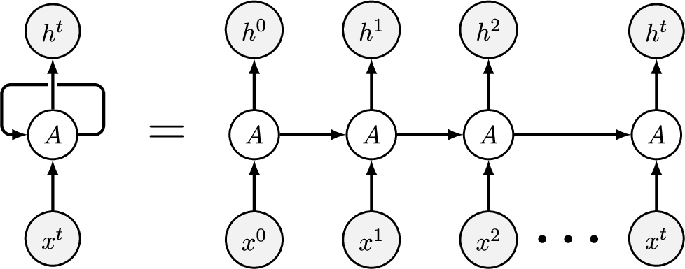
Neural networks (NNs) have a general functional definition as composition of parametric functions which disaggregates the linear component of the non-linear activation function (see García Cabello, 2023). Recurrent Neural networks, RNNs (Chou et al., 2022; Zhang et al., 2014), are a particular case of NNs which operate on time sequences and exhibit a special ability for learning lengthy-time period dependencies. Their functioning lies in an intermediary layer
(2)
The loss function
Fig. 1
RNN learning process.
3Problem Formulation
In this section we will develop the theoretical framework that will capacitate Markov Network-methodology to perform discriminative tasks based on prior probability and the VNM Theorem 2.1. Specifically, our aim is to design a mathematical model which enables MNs to identify the optimal RNN training sets, i.e. those that produce better estimates in forecasting taks. For a better understanding, we will make reference to a real example of a RNN forecasting process:
Recall that, in the networks as a whole, Recurrent Neural Networks, RNNs, stand out for their predictive abilities based on their potential in processing temporal data. Thus, we are facing some time-dependent learning process by using RNNs where the superscript t denotes time in all cases (no distinction will be made between matrices and their transpose in order to avoid confusion between t transpose and t time).
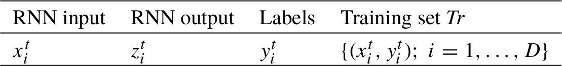
As is well known, in RNN prediction tasks, training sets are fed with temporal sequences composed with pairs of previous data of the form (input, labels) with the objective of predicting the future, referred to as future target value, y. Thus,
Let
The objective is to select from the n inputs in
We will list the steps to be taken:
• Main lottery (in
• Consider the RNN process as composed by several uncertain processes,
• Secondary lottery (for each
To ensure that our selection rule is applied, we define a preference relation on
In later sections we will show that this preference relation verifies the properties necessary for the application of the VNM theorem.Definition 3.1.
For
• We thus apply Theorem 2.1 for the main lottery: the expected utility of training set
(3)
• In order to compute the (prior) probabilities
• In order to compute the utility
4The Abstract TD-MRF-Based Framework
Here, we first design an abstract graph-based framework that shall provide a model for a dynamic context of k sites and r filters for data discrimination (corresponding to r cliques) for which it will be shown that it is an TD-MRF under certain mild conditions. Such TD-MRF will be the core in the computation of prior probabilities
Let
Remember that two random variables are equivalent if they have identical distribution. Then, we will define the edges by equivalently defining the neighbourhood
Definition 4.1
Definition 4.1(TD-DGM).
A DGM
Remark 4.2
Remark 4.2(Clean data).
It is worth highlighting that Definition 4.1 (that makes equal all random variables with identical probability distribution) avoids duplicates. This is particularly important when applied to the graphical model resulting from an RNN input dataset (clean data).
Recall that marginal distribution is also known as prior probability in contrast with the posterior distribution (the conditional one). From the former definition, sites in the same neighbourhood have the same prior probability. Moreover,
Proposition 4.3.
Sites which belong to the same neighbourhood have identical probability a posteriori.
Proof.
Let 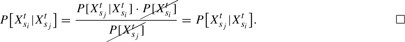
The following theorem proves then that the DGM defined in Definition 4.1 is a TD-MRF by equivalently showing that the Markov condition:
Proof.
We shall prove that the local dynamic Markov property is verified, i.e. the probability of
Insofar as the distribution function is the tool used to make estimates, previous Theorem 4.4 provides a joint measure of how close the variable is to taking a particular value.
Corollary 4.5.
The corresponding Gibbs (joint) probability distribution at a time instant t provides that the likelihood of reaching a concrete value x is
Remark 4.6.
Under Definition 4.1, neighbours and cliques are essentially the same and equal to the set of random variables with identical prior distribution. Moreover, according to Proposition 4.3, variables in a clique have also the same posterior distribution.
Each clique has its own common estimation function:
Proposition 4.7
Proposition 4.7(The cliques).
Each clique of the TD-MRF has its own estimation function given by the clique potentials
Proof.
It is straightforward from definition of clique. □
In discrimination/classification works, the commonly used probability is the conditional or posterior probability
4.1Visual Flowchart of the TD-MRF Operational Process
Inputs for a TD-MFRs are specific values of the stochastic variable
Fig. 2
TD-MRF operational process.
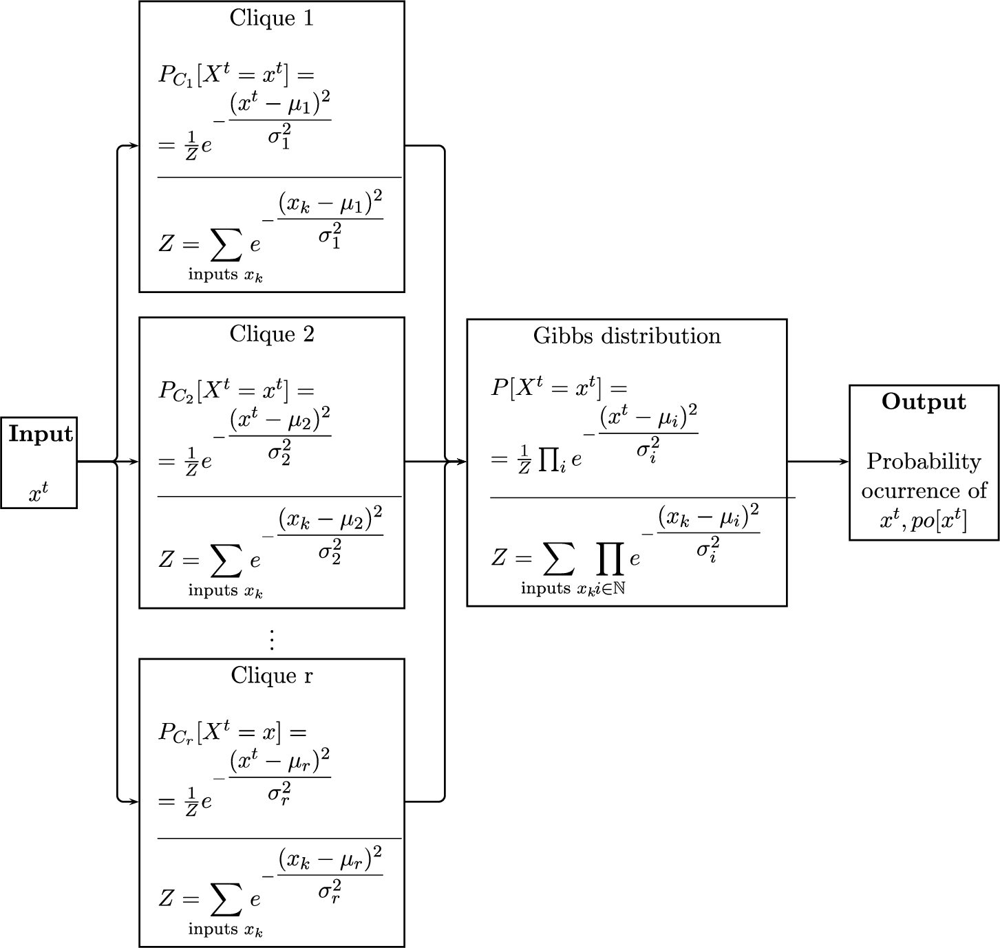
Figure 2 provides a visual representation of a TD-MRF operation in the univariate scenario, where the energy functions ψ are of Gaussian type, i.e.
Moreover, the operation of an MRF is equally applied in the calculation of following probabilities:
4.2TD-MRF Structure for the RNN Input Set
Our goal here is to provide a graph-structure (which will become TD-MRF structure according to Theorem 4.4) for the set
To achieve this, the steps to follow are listed below:
1. The pre-processing phase. Before training/testing an RNN, data must suffer some preprocessing steps for removing duplicates, unnecessary information and simulating missing data. Depending on the context, data must also be normalised with feature scaling. We shall assume that RNN input datasets have completed this phase.
2. The input set graph structure. We endow the RNN data set with an undirected graph structure, according to Definition 4.1, where
• sites
• The neighbourhood of a site is defined as
in the sense of Definition 4.1. According to Remark 4.2, this definition is intended for discarding duplicates in the datasets.
3. The corresponding Gibbs distribution. According to Theorem 4.4, the graphical model formed by the RNN input data viewed as a time varying random variable
4. Likelihood of occurrence of an output. Recall that from Definition 4.1, neighbours are equal to cliques and both consist of those random variables which have equal prior distributions (and identical posterior distribution in consequence). Hence, a probability
Note that the deterministic nature of RNN, which always assigns the same
5Application of the VNM Utility Theorem
In this section, we will further develop equation (3),
Recall that in the preceding sections we have considered a second lottery which arises naturally when we test how good the ouput
First of all, it has to be shown that it is a preference relation:
Proposition 5.1.
The relation defined in Definition 3.1 is a preference relation.
Proof.
The standard axiom for a preference relation is rationality which includes both completeness and transitivity.
• Completeness: for all
• Transitivity: for all
Moreover, former preference relation satisfies the following conditions:
Proposition 5.2.
The preference relation in Definition 3.1 satisfies:
• Continuity: if
• Fréchet differentiable: the functional form which defines de preferences (the loss function) must be Fréchet differentiable.
Proof.
Continuity: let us prove that if each element
Let us suppose that
By assuming that both limits exist, the inequality
Fréchet differentiable. Recall that the Fréchet derivative in finite-dimensional spaces is the usual derivative. Thus, the loss function
Therefore, the preference relation stated in Definition 3.1 verifies the conditions required for the application of the VNM Theorem 2.1. Thus, there exists an utility function
6Main Results
The objective of this section is to highlight (after proving) the main results of our proposal. First of all, we define the level of efficiency of an input set
Definition 6.1.
We define the level of efficiency of an input set
Theorem 6.2
Theorem 6.2(Existence).
For any input set
Proof.
Following Proposition 5.2, the preference relation stated in Definition 3.1 verifies the necessary conditions for applying the VNM Theorem 2.1. According to this, there exists an utility function
Theorem 6.3
Theorem 6.3(How to compute the level of efficiency of In
We assume that all inputs are equally distributed. Thus, for any RNN input set
Proof.
We start from expression
7A Case Application
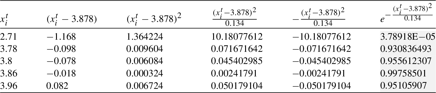
This section is aimed at developing an example of the method application. In order to make a choice between two real data sets, their level of efficiency will be computed. As stated in Definition 6.1, the level of efficiency of an input set
The data sets we shall use here contain prices (€/1 kg) over time for the most common olive oil varieties. These data are available on the websites of the Government of Spain:
where prices are published on a weekly basis. Specifically, we will consider data sets corresponding to weeks 28/2023 and 39/2022 (the reasons for this choice will be explained later). We shall thus apply the above formula taking into account the following considerations. On one hand, note that the choice of the threshold M will depend on the context. In the olive oil market scenario, assuming a deviation from the olive oil price of 10% is acceptable. Hence,
From the above formula, since M is known (and therefore so is p), we must focus on computing
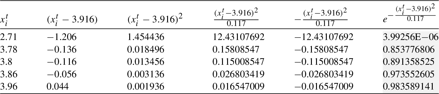
We assume that the energy functions ψ corresponding to the r cliques are of Gaussian type, i.e.
In order to achieve our goal, each input
From the TD-MRF structure proved in Theorem 4.4, cliques gather those random variables with identical prior and posterior distribution (see Remark 4.6). This theoretical description fits with the specialist major retailers in the olive oil context. In this practical case, the level of efficiency shall be computed through
Table 1
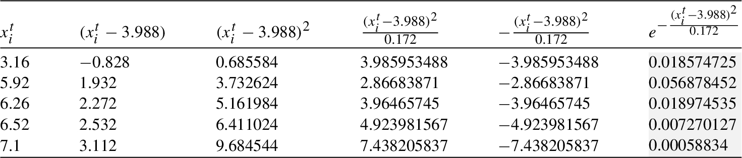
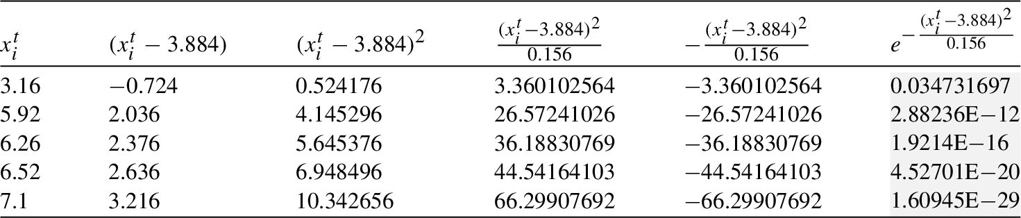
Table 2
As discussed before, there are multiple factors (physical and socio-economic) that influence the price. Such factors are the features
The computation of level of efficiency
Table 3
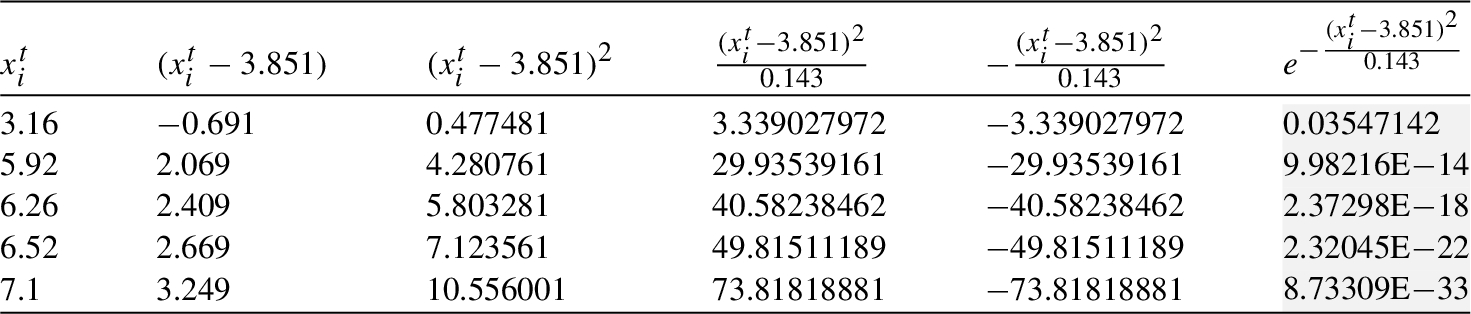
Table 4
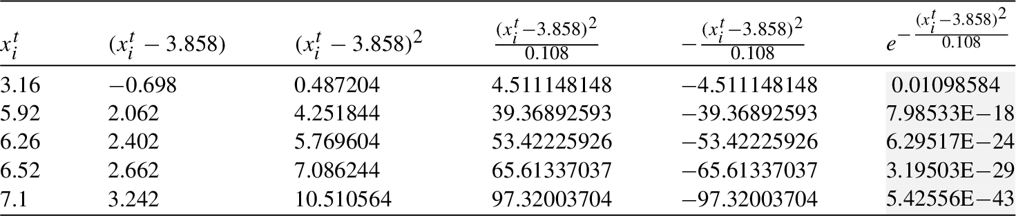
Table 5
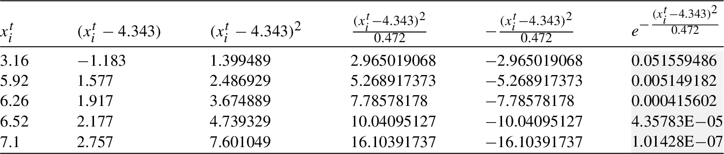
Table 6
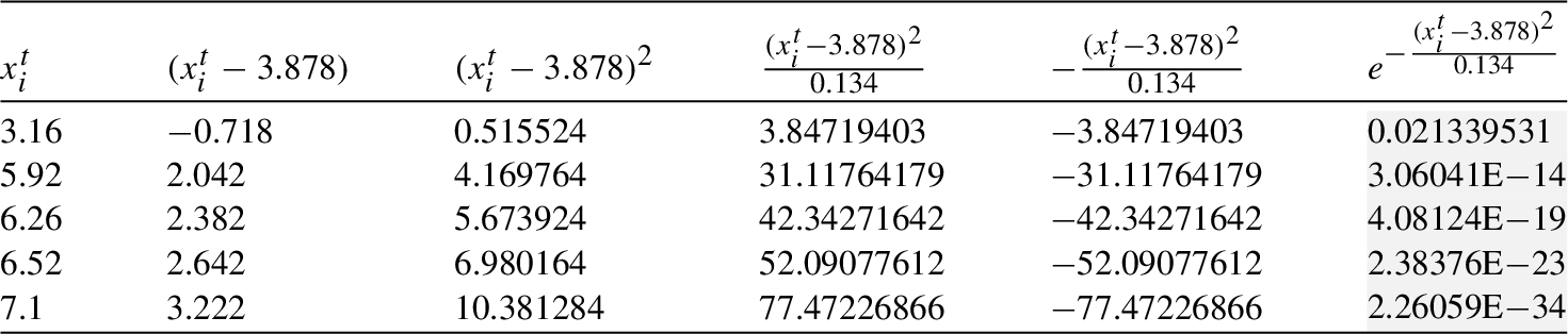
Table 7
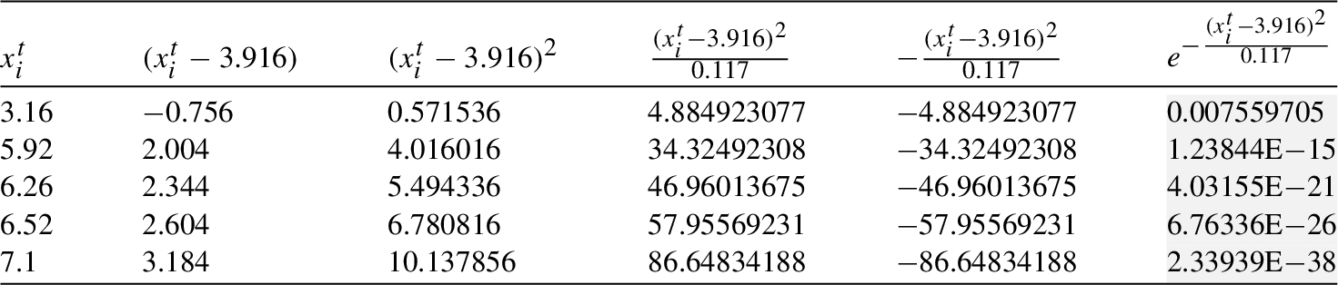
Table 8
Mean and variance of cliques
| Mean, Variance | |||||||
| 3.988 | 3.884 | 3.851 | 3.858 | 4.343 | 3.878 | 3.916 | |
| 0.172 | 0.156 | 0.143 | 0.108 | 0.472 | 0.134 | 0.117 |
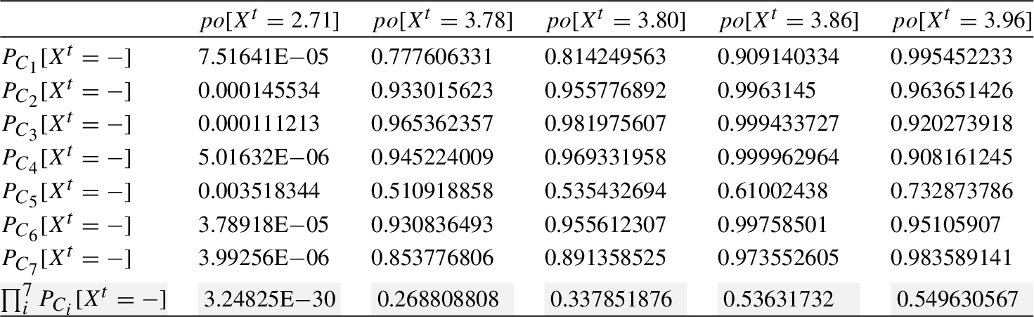
From the information provided by the above tables, finally the required probability is computed (see Table 9).
Table 9
Aggregated probability for
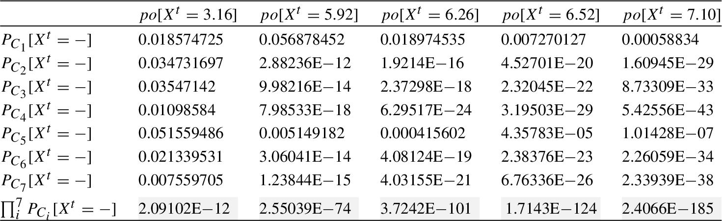
Similarly, the computation of
Table 10
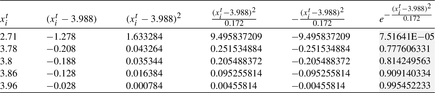
Table 11
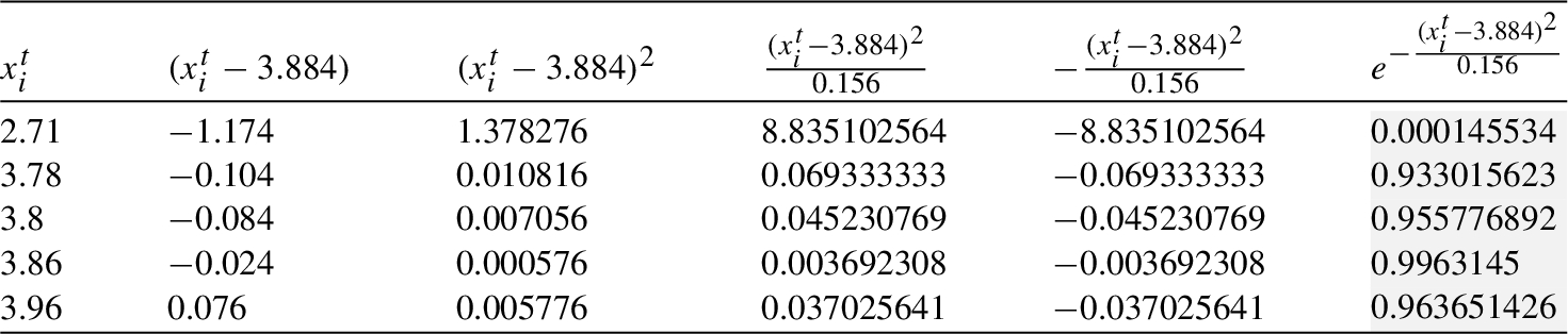
Table 12
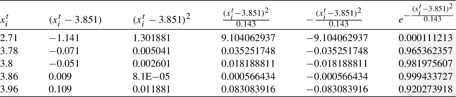
Table 13
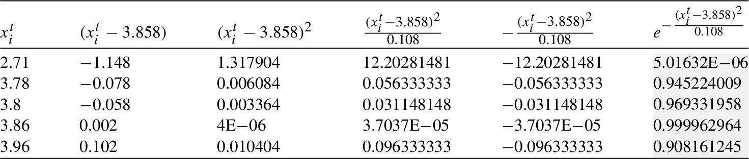
Table 14
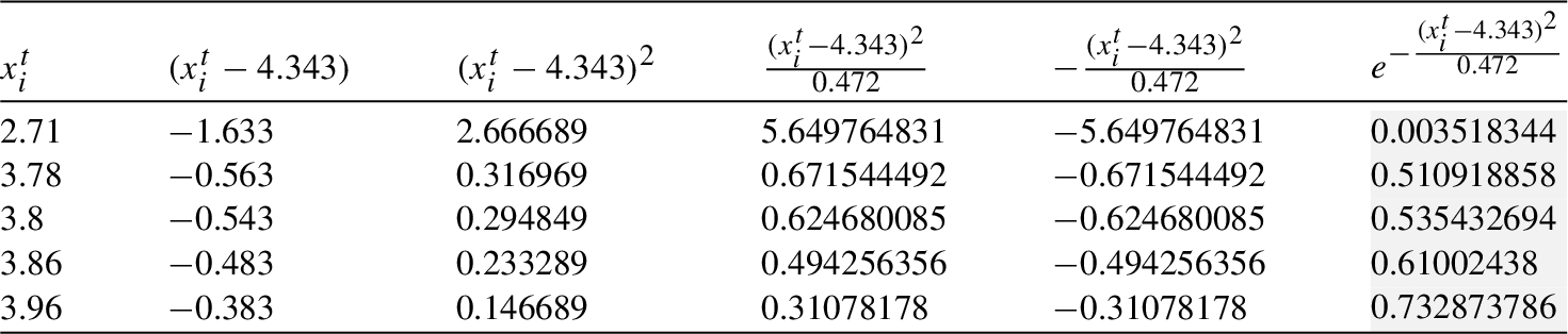
Table 15
Finally, the required probability is computed (see Table 17).
Table 16
 .
.
Table 17
Aggregated probability for
Hence, as expected (since the inputs of
8Conclusions
This paper deals with the selection of optimal training sets (those that have a higher capacity as estimators) in Recurrent Neural Networks under prediction tasks (or pattern recognition with time series as inputs), although this may also apply to other data-driven models regulated by dynamic systems. Our objective is to fill the existing gap of clear guidelines to follow for selecting optimal training sets in a general context.
We design here a novel methodology to select optimal training data sets that can be used in any context. The key idea, which underpins the design of the mathematical structure that supports the selection, is a binary relation that gives preference to inputs with higher estimator abilities. A second novelty of our approach is to use dynamic tools that have not been used previously for this purposes: dynamic Markov Networks, which are widely regarded as generative models, successfully compute the prior probabilities involved in the formula for calculating the degree of efficiency of the training set (Theorem 6.3), derived from application of the Von Neumann-Morgenstern Theorem 2.1. It is precisely the VMN theorem the instrument that confers discriminative capacity to the MNs: in this work we show that the preference relation that we define between inputs of a training set (inputs with higher learning capacities are preferred in the sense that the error function takes lower values) fulfils the necessary hypotheses to derive the existence of a simple formula for the calculation of the utility (efficiency) of a training set.
The simplicity of this calculation allows it to be carried out in parallel with the learning process without adding computational cost. Thus the optimal sets are selected as the learning process evolves, therefore the data noise gradually disappears which decreases the likelihood of overfitting occurring.
Declarations of interest: none.
Notes
1 Overfitting in data-driven learning models (which extract a predictive model from a data set) is the flaw of failing to generalise the features/patterns present in the training dataset. It occurs in models which extract features from datasets having too much noise.
2 We are using the term “site” instead of node for its additional connotation of location, which allows us to simulate that each of the nodes is a different geographical place that could generate its own estimate of the variable as explained below, in Proposition 4.7.
3 In dry seasons, water shortages lead to a drop in the olive production and, therefore, in the olive oil production. Hence, under severe drought conditions, olive oil prices skyrocket.
References
1 | Chen, A.N. ((2006) ). Robust optimization for performance tuning of modern database systems. European Journal of Operational Research, 171: , 412–429. https://doi.org/10.1016/j.ejor.2011.03.043. |
2 | Chou, P., Chuang, H.H., Chou, Y., Liang, T. ((2022) ). Predictive analytics for customer repurchase: Interdisciplinary integration of buy till you die modeling and machine learning. European Journal of Operational Research, 296: , 635–651. https://doi.org/10.1016/j.ejor.2021.04.021. |
3 | Delbaen, F., Drapeau, S., Kupper, M. ((2011) ). A von neumann morgenstern representation result without weak continuity assumption. Journal of Mathematical Economics, 47: , 401–408. https://doi.org/10.1016/j.jmateco.2011.04.002. |
4 | Dynkin, E. ((1984) ). Gaussian and nongaussian random fields associated with markov processes. Journal of Functional Analysis, 55: , 344–376. https://doi.org/10.1016/0022-1236(84)90004-1. |
5 | Fernandez Anitzine, I., Romo Argota, J.A., Fontan, F.P. (2012). Influence of training set selection in artificial neural network based propagation path loss predictions. International Journal of Antennas and Propagation, 2012. https://doi.org/10.1155/2012/351487. |
6 | García Cabello, J. ((2021) ). A novel intelligent system for securing cash levels using markov random fields. International Journal of Intelligent Systems, 36: , 4468–4490. https://doi.org/10.1002/int.22467. |
7 | García Cabello, J. (2023). Improved deep neural network performance under dynamic programming mode. Preprint. https://doi.org/10.2139/ssrn.4410415. |
8 | Gordon, J., Hernandez-Lobato, J.M. ((2020) ). Combining deep generative and discriminative models for bayesian semi-supervised learning. Pattern Recognition, 100: , 107156. https://doi.org/10.1016/j.patcog.2019.107156. |
9 | Higham, C.F., Higham, D.J. ((2019) ). Deep learning: an introduction for applied mathematicians. Siam Review, 61: , 860–891. https://doi.org/10.1137/18M1165748. |
10 | Jiang, L., Liao, H. ((2022) ). Bounded rational reciprocal preference relation for decision making. Informatica, 33: , 731–748. https://doi.org/10.15388/23-INFOR511. |
11 | Kim, K. ((2006) ). Artificial neural networks with evolutionary instance selection for financial forecasting. Expert Systems with Applications, 30: , 519–526. https://doi.org/10.1016/j.eswa.2005.10.007. |
12 | Machina, M.J. ((1982) ). Expected utility analysis without the independence axiom. Econometrica: Journal of the Econometric Society, 50: (2), 277–323. https://doi.org/10.2307/1912631. |
13 | Mirjalili, S., Hashim, S.Z.M., Sardroudi, H.M. ((2012) ). Training feedforward neural networks using hybrid particle swarm optimization and gravitational search algorithm. Applied Mathematics and Computation, 218: , 11125–11137. https://doi.org/10.1016/j.amc.2012.04.069. |
14 | Nalepa, J., Myller, M., Piechaczek, S., Hrynczenko, K., Kawulok, M. ((2018) ). Genetic selection of training sets for (not only) artificial neural networks. In: Kozielski, S., Mrozek, D., Kasprowski, P., Małysiak-Mrozek, B., Kostrzewa, D. (Eds.), Beyond Databases, Architectures and Structures. Facing the Challenges of Data Proliferation and Growing Variety, BDAS 2018, Communications in Computer and Information Science, Vol. 928: . Springer, Cham. https://doi.org/10.1007/978-3-319-99987-6_15. |
15 | Pollak, R.A. ((1967) ). Additive von neumann-morgenstern utility functions. Econometrica, Journal of the Econometric Society, 35: 3–4, 485–494. https://doi.org/10.2307/1905650. |
16 | Reeves, C.R., Bush, D.R. ((2001) ). Using genetic algorithms for training data selection in RBF networks. In: Liu, H., Motoda, H. (Eds.), Instance Selection and Construction for Data Mining, The Springer International Series in Engineering and Computer Science, 608: . Springer, Boston, MA, pp. 339–356. https://doi.org/10.1007/978-1-4757-3359-4_19. |
17 | Reeves, C.R., Taylor, S.J. ((1998) ). Selection of training data for neural networks by a genetic algorithm. In: Parallel Problem Solving from Nature-PPSN V: 5th International Conference Amsterdam, The Netherlands September 27–30, 1998 Proceedings 5. Springer, pp. 633–642. https://doi.org/10.1007/BFb0056905. |
18 | Smale, S., Rosasco, L., Bouvrie, J., Caponnetto, A., Poggio, T. ((2010) ). Mathematics of the neural response. Foundations of Computational Mathematics, 10: , 67–91. https://doi.org/10.1007/s10208-009-9049-1. |
19 | Van Den Brink, R., Rusinowska, A. ((2022) ). The degree measure as utility function over positions in graphs and digraphs. European Journal of Operational Research, 299: , 1033–1044. https://doi.org/10.1016/j.ejor.2021.10.017. |
20 | Wang, L., Zhou, Y., Li, R., Ding, L. ((2022) ). A fusion of a deep neural network and a hidden markov model to recognize the multiclass abnormal behavior of elderly people. Knowledge-Based Systems, 252: , 109351. https://doi.org/10.1016/j.knosys.2022.109351. |
21 | Wong, D.F., Lu, Y., Chao, L.S. ((2016) ). Bilingual recursive neural network based data selection for statistical machine translation. Knowledge-Based Systems, 108: , 15–24. https://doi.org/10.1016/j.knosys.2016.05.003. |
22 | Yang, J., Qiu, W. ((2005) ). A measure of risk and a decision-making model based on expected utility and entropy. European Journal of Operational Research, 164: , 792–799. https://doi.org/10.1016/j.ejor.2004.01.031. |
23 | Zapf, F., Wallek, T. ((2021) ). Comparison of data selection methods for modeling chemical processes with artificial neural networks. Applied Soft Computing, 113: , 107938. https://doi.org/10.1016/j.asoc.2021.107938. |
24 | Zhang, H., Wang, Z., Liu, D. ((2014) ). A comprehensive review of stability analysis of continuous-time recurrent neural networks. IEEE Transactions on Neural Networks and Learning Systems, 25: , 1229–1262. https://doi.org/10.1109/TNNLS.2014.2317880. |
25 | Zhang, L., Suganthan, P.N. ((2016) ). A survey of randomized algorithms for training neural networks. Information Sciences, 364: , 146–155. https://doi.org/10.1016/j.ins.2016.01.039. |


