Circular Pythagorean Fuzzy Sets and Applications to Multi-Criteria Decision Making

Bozyigit, Mahmut Can; Olgun, Murat; Ünver, Mehmet

doi:10.15388/23-INFOR529

Circular Pythagorean Fuzzy Sets and Applications to Multi-Criteria Decision Making

Article type: Research Article

Authors: Bozyigit, Mahmut Can¹ | Olgun, Murat² | Ünver, Mehmet^{2; ∗}

Affiliations: [1] Faculty of Engineering and Natural Sciences, Department of Mathematics, Ankara Yıldırım Beyazıt University, 06420 Ankara, Türkiye | [2] Faculty of Science, Department of Mathematics, Ankara University, 06100 Ankara, Türkiye

Correspondence: [∗] Corresponding author.

Keywords: circular Pythagorean fuzzy set, aggregation operators, multi-criteria decision making

DOI: 10.15388/23-INFOR529

Journal: Informatica, vol. 34, no. 4, pp. 713-742, 2023

Received October 2022

Accepted September 2023

Published: 2023

Get PDF

Abstract

In this paper, we introduce the concept of circular Pythagorean fuzzy set (value) (C-PFS(V)) as a new generalization of both circular intuitionistic fuzzy sets (C-IFSs) proposed by Atannassov and Pythagorean fuzzy sets (PFSs) proposed by Yager. A circular Pythagorean fuzzy set is represented by a circle that represents the membership degree and the non-membership degree and whose centre consists of non-negative real numbers μ and ν with the condition μ2+ν2⩽1. A C-PFS models the fuzziness of the uncertain information more properly thanks to its structure that allows modelling the information with points of a circle of a certain centre and a radius. Therefore, a C-PFS lets decision makers to evaluate objects in a larger and more flexible region and thus more sensitive decisions can be made. After defining the concept of C-PFS we define some fundamental set operations between C-PFSs and propose some algebraic operations between C-PFVs via general triangular norms and triangular conorms. By utilizing these algebraic operations, we introduce some weighted aggregation operators to transform input values represented by C-PFVs to a single output value. Then to determine the degree of similarity between C-PFVs we define a cosine similarity measure based on radius. Furthermore, we develop a method to transform a collection of Pythagorean fuzzy values to a C-PFS. Finally, a method is given to solve multi-criteria decision making problems in circular Pythagorean fuzzy environment and the proposed method is practiced to a problem about selecting the best photovoltaic cell from the literature. We also study the comparison analysis and time complexity of the proposed method.

1Introduction

The concept of fuzzy set (FS) was developed by utilizing a function (called membership function) assigning a value between zero and one as the membership degrees of the elements to deal with ambiguity in real-life problems. Since the FS theory proposed by Zadeh (1965) succeeded to handle various types of uncertainty, it has been studied in detail by many researchers to model uncertainty. Later, the concept of intuitionistic fuzzy set (IFS), which is an extension of the concept of FS, was proposed by Atanassov (1986) via membership functions and non-membership functions. The theory of IFS plays an important role in many research areas such as pattern recognition, multi-criteria decision making (MCDM), data mining, classification, clustering and medical diagnosis. Many aggregation operators and information measures (similarity, distance and entropy measures) have been developed for IFSs. Particularly, various generalizations of aggregation operators and information measures for IFSs (see, e.g. Beliakov et al., 2011; Boltürk and Kahraman, 2022; Garg and Arora, 2021; Olgun et al., 2021b; Verma and Sharma, 2013; Wan and Dong, 2014) have been defined via particular types of triangular norms (t-norms) and triangular conorms (t-conorms).

The concept of Pythagorean fuzzy set (PFS), first introduced by Atanassov (1999) as IFS of type 2, has become a significant tool in MCDM, as illustrated in Fig. 1, and as acknowledged by Yager (2013a, 2013b) in subsequent research. A PFS is characterized via a membership function and a non-membership function such that the sum of the squares of these non-negative functions is less than 1. Moreover, a PFS has a quadratic form, which means a PFS expands the range of the change of membership degree and non-membership degree to the unit circle and so is more capable than an IFS in depicting uncertainty. Yager (2013a), Yager and Abbasov (2013) proposed some aggregation operators for PFSs. After that, Peng et al. (2017) presented the axiomatic definitions of distance measure, similarity measure and entropy measure for PFSs. Further studies on MCDM with fuzzy sets and aggregation operators can be found in Beliakov et al. (2007), Biswas and Sarkar (2018), Garg (2016), Garg and Arora (2021), Grabisch et al. (2009), Kahraman (2008), Olgun et al. (2019), Olgun et al. (2021a), Yeni and Özçelik (2019), Ünver et al. (2022a), Ünver et al. (2022b), Ye et al. (2022), Yolcu et al. (2021), Zhang and Xu (2014), Zeng et al. (2018).

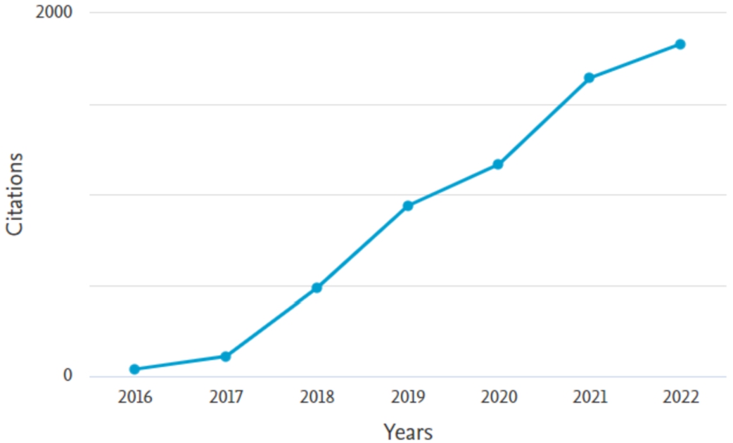
Fig. 1

Citation graph of the PFSs.

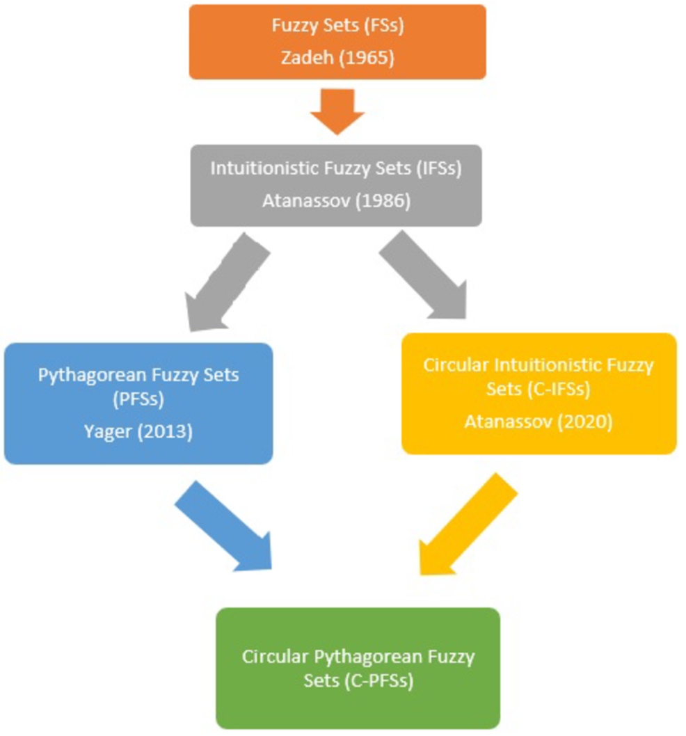
Many types of fuzzy sets study with points, pairs of points or triples of points from the closed interval [0,1] that makes the decision process stricter since they require decision makers (DMs) to assign precise numbers. To overcome such a strict modelling, Atanassov (2020) proposed the concept of circular intuitionistic fuzzy set (C-IFSs). A C-IFS is represented by a circle standing for the uncertainty of the membership and non-membership functions. That is, the membership and the non-membership of each element to a C-IFS are shown as a circle whose centre is a pair of non-negative real numbers with the condition that the sum of them is less than 1. With the help of C-IFSs, the change of membership degree and non-membership degree can be handled more sensitively to express uncertainty. Therefore, various types of MCDM methods have been carried to circular intuitionistic fuzzy environment (see e.g. Atanassov and Marinov, 2021; Kahraman and Alkan, 2021; Kahraman and Otay, 2022). In this paper, we carry the idea of representing membership degree and non-membership degree as circle to the Pythagorean fuzzy environment by introducing the concept of circular Pythagorean fuzzy set (C-PFS). In this new fuzzy set notion, the membership and non-membership degrees of an element to a FS are represented by circles with centre (μA(x),νA(x)) instead of numbers and with a more flexible condition μA2(x)+νA2(x)⩽1. In this manner, we extend not only the concept of the PFS, but also the concept of the C-IFS (see Fig. 2). Thus the decision making process becomes more sensitive since DMs can attain circles with certain properties instead of precise numbers. Figure 2 illustrates the improvement of circular fuzzy sets.

Fig. 2

The improvement of circular fuzzy set theory.

Some main contributions of the present paper can be given as follows.

• This paper introduces the concepts of C-PFS and circular Pythagorean fuzzy value (C-PFV).
• A method is developed to transform a collection of Pythagorean fuzzy values (PFVs) to a C-PFV. In this way, multi-criteria group decision making (MCGDM) problem can be relieved.
• The membership and non-membership of an element to a C-PFS are represented by circles. Thanks to its structure, a more sensitive modelling can be done in MCDM theory in the continuous environment.
• Some algebraic operations are defined for C-PFVs via t-norms and t-conorms. With the help of these operations, some weighted arithmetic and geometric aggregation operators are provided. These aggregation operators are used in MCDM and MCGDM.

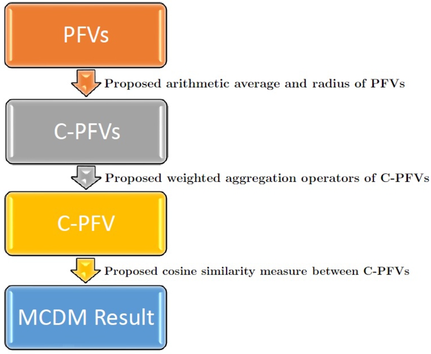
The rest of this paper is organized as follows. In Section 2, we recall some basic concepts. In Section 3, we introduce the concept of C-PFS(V) as new generalization of both C-IFSs and PFSs. We also define some fundamental set theoretic operations for C-PFSs. Then we introduce some algebraic operations for C-PFVs via continuous Archimedean t-norms and t-conorms. In Section 4, we propose some weighted aggregation operators for C-PFVs by utilizing these algebraic operations. In Section 5, motivated by a cosine similarity measure defined for PFVs in Wei and Wei (2018), we define a cosine similarity measure for C-PFVs to determine the degree of similarity between C-PFVs. Using the proposed similarity measure and the aggregation operators we provide an MCDM method in circular Pythagorean fuzzy environment. We also apply the proposed method to an MCDM problem from Zhang (2016) that deals with selecting the best photovoltaic cell (also known as solar cell). We compare the results of the proposed method with the existing result and calculate the time complexity of the MCDM method. In Section 6, we conclude the paper.

2Preliminaries

Atanassov (1986) introduced the concept of IFS by taking into account the non-membership functions with a membership functions of FSs. Throughout this section we assume that X={x1,…,xn} is a finite set.

Definition 1

Definition 1(Atanassov, 1986).

An IFS A in X is defined by

A={⟨x,μA(x),νA(x)⟩:x∈X},

where μA,νA:X→[0,1] are functions with the condition

μA+νA⩽1

that are called the membership function and the non-membership function, respectively.

The concept of PFS proposed by Yager (2013a, 2013b) which is a generalization of IFS.

Definition 2

Definition 2(Yager 2013a, 2013b).

A PFS A in X is defined by

A={⟨x,μA(x),νA(x)⟩:x∈X},

where μA,νA:X→[0,1] are functions with the condition

μA2+νA2⩽1

that are called themembership function and the non-membership function, respectively. Let μα,να∈[0,1] such that μα2+να2⩽1. Then the pair α=⟨μα,να⟩ is called a Pythagorean fuzzy value (PFV).

Schweizer and Sklar (1983) introduced the concepts of t-norm and t-conorm by motivating the concept of probabilistic metric spaces proposed by Menger (1942). These concepts have important roles in statistics and decision making. Algebraically, t-norms and t-conorms are binary operations defined on the closed unit interval.

Definition 3

Definition 3(Klement et al., 2002; Schweizer and Sklar, 1983).

A t-norm is a function T:[0,1]×[0,1]→[0,1] that satisfies the following conditions:

(T1) T(x,1)=x for all x∈[0,1] (border condition),
(T2) T(x,y)=T(y,x) for all x,y∈[0,1] (commutativity),
(T3) T(x,T(y,z))=T(T(x,y),z) for all x,y,z∈[0,1] (associativity),
(T4) T(x,y)⩽T(x′,y′) whenever x⩽x′ and y⩽y′ for all x,x′,y,y′∈[0,1] (monotonicity).

Definition 4

Definition 4(Klement et al., 2002; Schweizer and Sklar, 1983).

A t-conorm is a function S:[0,1]×[0,1]→[0,1] that satisfies the following conditions:

(S1) S(x,0)=x for all x∈[0,1] (border condition),
(S2) S(x,y)=S(y,x) for all x,y∈[0,1] (commutativity),
(S3) S(x,S(y,z))=S(S(x,y),z) for all x,y,z∈[0,1] (associativity),
(S4) S(x,y)⩽S(x′,y′) whenever x⩽x′ and y⩽y′ for all x,x′,y,y′∈[0,1] (monotonicity).

Definition 5

Definition 5(Klement et al. 2002, 2004a).

A strictly decreasing function g:[0,1]→[0,∞] with g(1)=0 is called the additive generator of a t-norm T if we have T(x,y)=g−1(g(x)+g(y)) for all (x,y)∈[0,1]×[0,1].

Next, we need the concept of fuzzy complement to find the additive generator of a dual t-conorm on [0,1].

Definition 6

Definition 6(Yager 2013a, 2013b; Yang et al., 2019).

A fuzzy complement is a function N:[0,1]→[0,1] satisfying the following conditions:

(N1) N(0)=1 and N(1)=0 (boundary conditions),
(N2) N(x)⩾N(y) whenever x⩽y for all x,y∈[0,1] (monotonicity),
(N3) Continuity,
(N4) N(N(x))=x for all x∈[0,1] (involution).

The function N:[0,1]→[0,1] defined by N(a)=(1−ap)1/p, where p∈(0,∞) (Yager 2013a, 2013b) is a fuzzy complement. When p=2, N becomes the Pythagorean fuzzy complement N(a)=1−a2.

Definition 7

Definition 7(Klir and Yuan, 1995; Yang et al., 2019).

Let T be a t-norm and let S be a t-conorm on [0,1]. If T(x,y)=N(S(N(x),N(y))) and S(x,y)=N(T(N(x),N(y))), then T and S are called dual with respect to a fuzzy complement N.

Remark 1.

Let T be a t-norm on [0,1]. Then the dual t-conorm S with respect to the Pythagorean fuzzy complement N is

S(x,y)=1−T2(1−x2,1−y2).

Note that T is an Archimedean t-norm if and only if T(x,x)<x for all x∈(0,1) and S is an Archimedean t-conorm if and only if S(x,x)>x for all x∈(0,1) (Klement et al. 2002, 2004a). Klement et al. (2004b) proved that continuous Archimedean t-norms have representations via their additive generators in the following theorem.

Theorem 1

Theorem 1(Klement et al., 2004b).

Let T be a t-norm on [0,1]. The following statements are equivalent:

(i) T is a continuous Archimedean t-norm.
(ii) T has a continuous additive generator, i.e. there is a continuous, strictly decreasing function g:[0,1]→[0,∞] with t(1)=0 such that T(x,y)=g−1(g(x)+g(y)) for all (x,y)∈[0,1]×[0,1].

3Circular Pythagorean Fuzzy Sets

The notion of C-IFS was introduced by Atanassov (2020) as an extension of the notion of IFS. Throughout this paper we assume that X={x1,…,xn} is a finite set.

Definition 8

Definition 8(Atanassov, 2020).

Let r∈[0,1]. A circular C-IFS Ar in X is defined by

Ar={⟨x,μA(x),νA(x);r⟩:x∈X},

where μA,νA:X→[0,1] are functions such that

μA+νA⩽1.

r is the radius of the circle around the point (μA(x),νA(x)) on the plane. This circle represents the membership degree and non-membership degree of x∈X.

Remark 2.

Since each IFS A has the form

A=A0={⟨x,μA(x),νA(x);0⟩:x∈X},

any IFS can be considered as a C-IFS. Hence, the notion of C-IFS is a generalization of the notion of IFS.

Next, we introduce the concept of C-PFS that is a new extension of the concepts of C-IFS and PFS. C-PFSs allow decision makers to express uncertainty via membership and non-membership degrees represented by a circle in a more extended environment. Thus, more sensitive evaluations can be made in decision making process.

Definition 9.

Let r∈[0,1]. A C-PFS Ar in X is defined by

Ar={⟨x,μA(x),νA(x);r⟩:x∈X},

where μA,νA:X→[0,1] are functions such that

μA2+νA2⩽1.

r is the radius of the circle around the point (μA(x),νA(x)) on the plane. This circle represents the membership degree and non-membership degree of x∈X.

Example 1.

Let X={x1,x2,x3}. An example of a C-PFS on X can be given by

A0.2={⟨x1,0.3,0.8;0.2⟩,⟨x2,0.1,0.9;0.2⟩,⟨x3,0.5,0.6;0.2⟩}.

Definition 10.

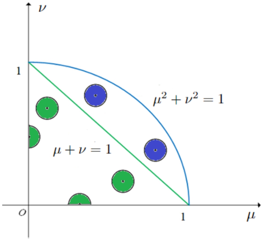
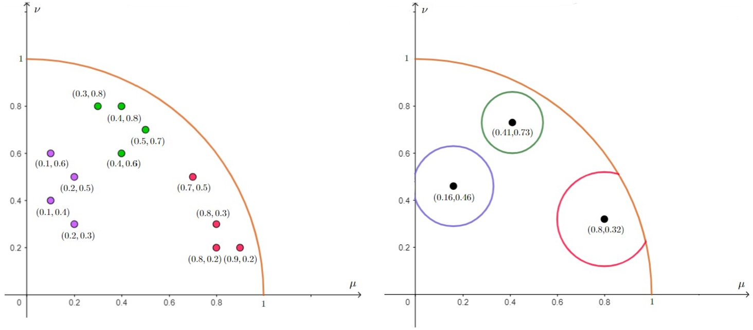
Let μα,να∈[0,1], such that μα2+να2⩽1 and rα∈[0,1]. Then the triple α=⟨μα,να;rα⟩ is called a C-PFV.

A C-PFS can be considered as a collection of C-PFVs. Figure 3 shows some examples of C-PFVs and Fig. 4 shows that the concept of C-PFS generalizes the concept of C-IFS.

Fig. 3

Geometric representation of C-PFSs.

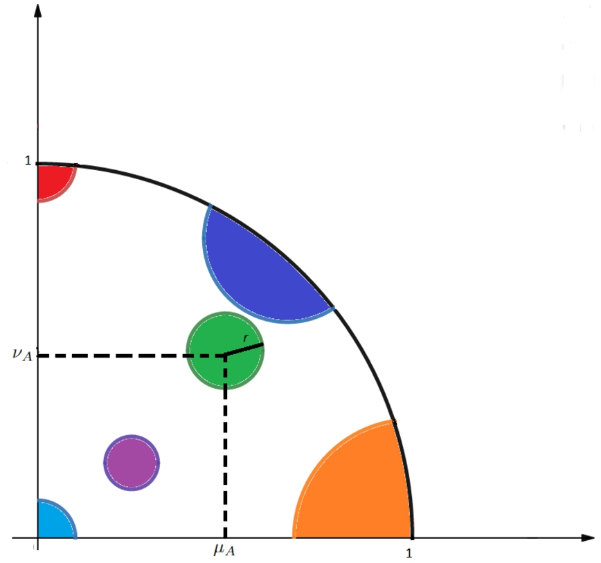
Fig. 4

Comparison of the spaces of C-IFS and C-PFS.

Remark 3.

Since each PFS A has the form

A=A0={⟨x,μA(x),νA(x);0⟩:x∈X},

any PFS is also a C-PFS but the converse is not true in general. Consider the C-PFS A0.2 given in Example 1. Since 0.3+0.8=1.1>1, it is not a C-IFS.

Now we can define some set operations among C-PFSs.

Definition 11.

Let

Ar={⟨x,μA(x),νA(x);r⟩:x∈X}

and

Bs={⟨x,μB(x),νB(x);s⟩:x∈X}

be two C-PFSs in X. Some set operations among C-PFSs are defined as follows:

a) Ar⊂Bs if and only if r⩽s and
μA(x)⩽μB(x)andνA(x)⩾νB(x),for anyx∈X.
b) Ar=Bs if and only if r=s and
μA(x)=μB(x)andνA(x)=νB(x),for anyx∈X.
c) The complement Arc of Ar is defined by Arc={⟨x,νA(x),μA(x);r⟩:x∈X}.
d) The union of Ar and Bs with respect to maximum and minimum is defined by
Ar∪minBs={⟨x,max(μA(x),μB(x)),min(νA(x),νB(x));min(r,s)⟩:x∈X}
and
Ar∪maxBs={⟨x,max(μA(x),μB(x)),min(νA(x),νB(x));max(r,s)⟩:x∈X},
respectively.
e) The intersection of Ar and Bs with respect to maximum and minimum is defined by
Ar∩minBs={⟨x,min(μA(x),μB(x)),max(νA(x),νB(x));min(r,s)⟩:x∈X}
and
Ar∩maxBs={⟨x,min(μA(x),μB(x)),max(νA(x),νB(x));max(r,s)⟩:x∈X},
respectively.

Example 2.

Let X={x1,x2,x3}. Consider the C-PFSs given with

A0.2={⟨x1,0.3,0.8;0.2⟩,⟨x2,0.1,0.9;0.2⟩,⟨x3,0.5,0.6;0.2⟩}

and

B0.6={⟨x1,0.7,0.5;0.6⟩,⟨x2,0.2,0.5;0.6⟩,⟨x3,0.6,0.3;0.6⟩}.

Then A0.2⊂B0.6. On the other hand,

A0.2c={⟨x1,0.8,0.3;0.2⟩,⟨x2,0.9,0.1;0.2⟩,⟨x3,0.6,0.5;0.2⟩},A0.2∪minB0.6={⟨x1,0.7,0.5;0.2⟩,⟨x2,0.2,0.5;0.2⟩,⟨x3,0.6,0.3;0.2⟩},A0.2∪maxB0.6={⟨x1,0.7,0.5;0.6⟩,⟨x2,0.2,0.5;0.6⟩,⟨x3,0.6,0.3;0.6⟩},A0.2∩minB0.6={⟨x1,0.3,0.8;0.2⟩,⟨x2,0.1,0.9;0.2⟩,⟨x3,0.5,0.6;0.2⟩},

and

A0.2∩maxB0.6={⟨x1,0.3,0.8;0.6⟩,⟨x2,0.1,0.9;0.6⟩,⟨x3,0.5,0.6;0.6⟩}.

The following theorem shows that De Morgan’s rules are available for C-PFSs.

Theorem 2.

Let

Ar={⟨x,μA(x),νA(x);r⟩:x∈X}

and

Bs={⟨x,μB(x),νB(x);s⟩:x∈X}

be two C-PFSs in X. Then we have:

1) (Ar∪minBs)c=Aric∩minBsic;
2) (Ar∪maxBs)c=Aric∩maxBsic;
3) (Ar∩minBs)c=Aric∪minBsic;
4) (Ar∩maxBs)c=Aric∪maxBsic.

Proof.

The proof is trivial from Definition 11. □

Now we develop a method to convert collections of PFVs to a C-PFV which is a useful method in group decision making.

Proposition 1.

Let {⟨μ1,ν1⟩,⟨μ2,ν2⟩,…,⟨μk,νk⟩} be a collection of PFVs. Then

⟨μ,ν;r⟩

is a C-PFV where

μ=∑j=1kμj2k,ν=∑j=1kνj2k

and

r=min{max1⩽j⩽k(μ−μj)2+(ν−νj)2,1}.

Proof.

We have

μ2+ν2=(∑j=1kμj2k′,)2+(∑j=1kνj2k)2=∑j=1kμ,j2ki+∑j=1kνj2ki=∑j=1k(μ,j2+ν,j2)k⩽∑j=1k1k=1.

Furthermore, it is clear that 0⩽r⩽1. Therefore, Ar=⟨μ,ν;r⟩ is a C-PFV. □

Example 3.

We present the following collections of PFVs:

{⟨0.3,0.8⟩,⟨0.4,0.6⟩,⟨0.5,0.7⟩,⟨0.4,0.8⟩},{⟨0.2,0.3⟩,⟨0.1,0.4⟩,⟨0.2,0.5⟩,⟨0.1,0.6⟩},

and

{⟨0.9,0.2⟩,⟨0.8,0.3⟩,⟨0.8,0.2⟩,⟨0.7,0.5⟩}.

By applying Proposition 1, we derive the corresponding C-PFVs, respectively:

⟨0.41,0.73;0.13⟩,⟨0.16,0.46;0.17⟩

and

⟨0.8,0.32;0.2⟩.

We visualize this transformations in Fig. 5.

Fig. 5

The PFVs and C-PFVs in Example 3.

Now we define some algebraic operations for C-PFVs.

Definition 12.

Let α=⟨μα,να;rα⟩ and β=⟨μβ,νβ;rβ⟩ be two C-PFVs. Some algebraic operations among C-PFVs are defined as follows:

a) α⊕minβ=⟨μα2+μβ2−μα2μβ2,ν1ν2;min(rα,rβ)⟩,
b) α⊕maxβ=⟨μα2+μβ2−μα2μβ2,ν1ν2;max(rα,rβ)⟩,
c) α⊗minβ=⟨μαμβ,να2+νβ2−να2νβ2;min(rα,rβ)⟩,
d) α⊗maxβ=⟨μαμβ,να2+νβ2−να2νβ2;max(rα,rβ)⟩.

Algebraic operations among C-PFVs in Definition 12 can be extended by using general t-norms and t-conorms.

Definition 13.

Let α=⟨μα,να;rα⟩ and β=⟨μβ,νβ;rβ⟩ be two C-PFVs. Assume that T,S are dual t-norm and t-conorm with respect to the Pythagorean fuzzy complement N(a)=1−a2, respectively, and Q is a t-norm or a t-conorm. General algebraic operations among C-PFVs are defined as follows:

a) α⊕Qβ=⟨S(μα,μβ),T(να,νβ);Q(rα,rβ)⟩,
b) α⊗Qβ=⟨T(μα,μβ),S(να,νβ);Q(rα,rβ)⟩.

It is clear that with a particular choice of S,T and Q the operations given in Definition 12 are obtained from the operations defined in Definition 13.

We now show that the sum and the product of two C-PFVs are also C-PFVs with the following proposition.

Proposition 2.

Let α and β be two C-PFVs. Assume that T,S are dual t-norm and t-conorm with respect to Pythagorean fuzzy complement N(a)=1−a2, respectively, and Q is a t-norm or a t-conorm. Then α⊕Qβ and α⊗Qβ are also C-PFVs.

Proof.

We know that the dual t-conorm S with respect to the Pythagorean fuzzy complement N is S(x,y)=1−T2(1−x2,1−y2) from Remark 1. Since μα⩽1−να2 and T is increasing, it is obtained that

T2(μα,μβ)+S2(να,νβ)=T2(μα,μβ)+(1−T2(1−να2,1−νβ2))2=T2(μα,μβ)+1−T2(1−να2,1−νβ2)⩽T2(1−να2,1−νβ2)+1−T2(1−να2,1−νβ2)=1.

Moreover, since the domain of Q is the unit closed interval we conclude that α⊗Qβ is a C-PFV. Similarly, it can be shown that α⊕Qβ is also a C-PFV. □

Klement et al. (2004b) showed that continuous Archimedean t-norms and t-conorms can be expressed with their additive generators. Thus, some algebraic operations among C-PFVs can be defined using additive generators of strict Archimedean t-norms and t-conorms.

Definition 14.

Let α=⟨μα,να;rα⟩ and β=⟨μβ,νβ;rβ⟩ be two C-PFVs and let λ>0. Assume that g:[0,1]→[0,∞] is the additive generator of a continuous Archimedean t-norm and h(t)=g(1−t2) and q:[0,1]→[0,∞] is the additive generator of a continuous Archimedean t-norm or t-conorm. Some algebraic operations among C-PFVs are defined as follows:

a) α⊕qβ=⟨h−1(h(μα)+h(μβ)),g−1(g(να)+g(νβ));q−1(q(rα)+q(rβ))⟩,
b) α⊗qβ=⟨g−1(g(μα)+g(μβ)),h−1(h(να)+h(νβ));q−1(q(rα)+q(rβ))⟩,
c) λqα=⟨h−1(λh(μα)),g−1(λg(να));q−1(λq(rα))⟩,
d) αλq=⟨g−1(λg(μα)),h−1(λh(να));q−1(λq(rα))⟩.

The following proposition confirms that multiplication by constant and power of C-PFVs are also C-PFVs.

Proposition 3.

Let α=⟨μα,να;rα⟩ and β=⟨μβ,νβ;rβ⟩ be two C-PFVs and let λ>0. Assume that g:[0,1]→[0,∞] is the additive generator of a continuous Archimedean t-norm and h(t)=g(1−t2) and q:[0,1]→[0,∞] is the additive generator of a continuous Archimedean t-norm or t-conorm. Then α⊕qβ, α⊗qβ, λqα and αλq are C-PFVs.

Proof.

It is clear from Proposition 2 that α⊕qβ and α⊗qβ are C-PFVs. We know that h−1(t)=1−[g−1(t)]2 and g(t)=h(1−t2). Since μα⩽1−να2 and h, h−1 are increasing, we have

0⩽[h−1(λh(μα))]2+[g−1(λg(να))]2⩽[h−1(λh(1−να2))]2+[g−1(λg(να))]2=1−[g−1(λh(1−να2)]2+[g−1(λg(να))]2=1−[g−1(λg(να))]2+[g−1(λg(να))]2=1.

Moreover, since the range of q−1 is the unit closed interval, we conclude that λqα is a C-PFV. In a similar way, it can be shown that αλq is also a C-PFV. □

Example 4.

Let g,h,q,p:[0,1]→[0,∞] defined by g(t)=−logt2, h(t)=−log(1−t2), q(t)=−logt2 and p(t)=−log(1−t2) and λ>0. Then we obtain the algebraic operators

a) α⊕qβ=⟨μα2+μβ2−μα2μβ2,νανβ;rαrβ⟩,
b) α⊕pβ=⟨μα2+μβ2−μα2μβ2,νανβ;rα2+rβ2−rα2rβ2⟩,
c) α⊗qβ=⟨μαμβ,να2+νβ2−να2νβ2;rαrβ⟩,
d) α⊗pβ=⟨μαμβ,να2+νβ2−να2νβ2;rα2+rβ2−rα2rβ2⟩,
e) λqα=⟨1−(1−μα2)λ,ναλ;rαλ⟩,
f) λpα=⟨1−(1−μα2)λ,ναλ;1−(1−rα2)λ⟩,
g) αλq=⟨μαλ,1−(1−να2)λ;rαλ⟩,
h) αλp=⟨μαλ,1−(1−να2)λ;1−(1−rα2)λ⟩.

The following theorem gives some basic properties of algebraic operations.

Theorem 3.

Let α=⟨μα,να;rα⟩, β=⟨μβ,νβ;rβ⟩ and θ=⟨μθ,νθ;rθ⟩ be C-PFVs and let λ,γ>0. Assume that g:[0,1]→[0,∞] is the additive generator of a continuous Archimedean t-norm and h(t)=g(1−t2) and q:[0,1]→[0,∞] is the additive generator of a continuous Archimedean t-norm or t-conorm. We have

i) α⊕qβ=β⊕qα,
ii) α⊗qβ=β⊗qα,
iii) (α⊕qβ)⊕qθ=α⊕q(β⊕qθ),
iv) (α⊗qβ)⊗qθ=α⊗q(β⊗qθ),
v) λq(α⊕qβ)=λqα⊕qλqβ,
vi) (λq+γq)α=λqα⊕qγqα,
vii) (α⊗qβ)λq=αλq⊗qβλq,
viii) αλq⊗qαγq=αλq+γq.

Proof.

(i) and (ii) are trivial.

iii) We obtain
(α⊕qβ)⊕qθ=⟨h−1(h(μα)+h(μβ)),g−1(g(να)+g(νβ));q−1(q(rα)+q(rβ))⟩⊕q⟨μθ,νθ;rθ⟩=⟨h−1(h(h−1(h(μα)+h(μβ))+h(μθ)),g−1(g(g−1(g(να)+g(νβ))+g(νθ));q−1(q(q−1(q(rα)+q(rβ))+q(rθ))⟩=⟨h−1(h(μα)+h(μβ)+h(μθ)),g−1(g(να)+g(νβ)+g(νθ));q−1(q(rα)+q(rβ)+q(rθ))⟩=⟨h−1(h(μα)+h(h−1(h(μβ)+h(μθ)))),g−1(g(να)+g(g−1(g(νβ)+g(νθ))));q−1(q(rα)+q(q−1(q(rβ)+q(rθ))))⟩=⟨μα,να;rα⟩⊕q⟨h−1(h(μβ)+h(μθ)),g−1(g(νβ)+g(νθ));q−1(q(rβ)+q(rθ))⟩=α⊕q(β⊕qθ).
iv) It is obtained that
(α⊗qβ)⊗qθ=⟨g−1(g(μα)+g(μβ)),h−1(h(να)+h(νβ));q−1(q(rα)+q(rβ))⟩⊗q⟨μθ,νθ;rθ⟩=⟨g−1(g(g−1(g(μα)+g(μβ))+g(μθ)),h−1(h(h−1(h(να)+h(νβ))+h(νθ));q−1(q(q−1(q(rα)+q(rβ))+q(rθ))⟩=⟨g−1(g(μα)+g(μβ)+g(μθ)),h−1(h(να)+h(νβ)+h(νθ));q−1(q(rα)+q(rβ)+q(rθ))⟩=⟨g−1(g(μα)+g(g−1(g(μβ)+g(μθ)))),h−1(h(να)+h(h−1(h(νβ)+h(νθ))));q−1(q(rα)+q(q−1(q(rβ)+q(rθ))))⟩=⟨μα,να;rα⟩⊗q⟨g−1(g(μβ)+g(μθ)),h−1(h(νβ)+h(νθ));q−1(q(rβ)+q(rθ))⟩=α⊗q(β⊗qθ).
v) We get
λq(α⊕qβ)=λq⟨h−1(h(μα)+h(μβ)),g−1(g(να)+g(νβ));q−1(q(rα)+q(rβ))⟩=⟨h−1(λh(h−1(h(μα)+h(μβ)))),g−1(λg(g−1(g(να)+g(νβ))));q−1(λq(q−1(q(rα)+q(rβ))))⟩=⟨h−1(λh(μα)+λh(μβ)),g−1(λg(να)+λg(νβ));q−1(λq(rα)+λq(rβ))⟩=⟨h−1(h(h−1(λh(μα)))+h(h−1(λh(μβ)))),g−1(g(g−1(λg(να))+g(g−1(λg(νβ))));q−1(q(q−1(λq(rα)))+q(q−1(λq(rβ))))⟩=⟨h−1(h(μλα)+h(μλβ)),g−1(g(νλα)+g(νλβ));q−1(q(rλα)+λq(sλβ))⟩=λqα⊕qλqβ.
vi) It is clear that
(λq+γq)α=⟨h−1((λ+γ)h(μα)),g−1((λ+γ)g(να));q−1((λ+γ)q(rα))⟩=⟨h−1(λh(μα)+γh(μα)),g−1(λg(να)+γg(να));q−1(λq(rα)+γq(rα))⟩=⟨h−1(h(h−1(λh(μα)))+h(h−1(γh(μα)))),g−1(g(g−1(λg(να)))+g(g−1(γg(να))));q−1(q(q−1(λq(rα)))+q(q−1(γq(rα))))⟩=⟨h−1(h(μλqα)+h(μγqα)),g−1(g(νλqα)+g(νγqα));q−1(q(rλqα)+q(rγqα))⟩=λqα⊕qγqα.
vii) We have
(α⊗qβ)λq=⟨g−1(λg(μα⊗qβ)),h−1(λh(να⊗qβ));q−1(λq(rα⊗qβ))⟩=⟨g−1(λg(g−1(g(μα)+g(μβ)))),h−1(λh(h−1(h(να)+h(νβ))));q−1(λq(q−1(q(rα)+q(rβ))))⟩=⟨g−1(λg(μα)+λg(μβ)),h−1(λh(να)+λh(νβ));q−1(λq(rα)+λq(rβ))⟩=⟨g−1(g(g−1(λg(μα)))+g(g−1(λg(μβ)))),h−1(h(h−1(λh(να)))+h(h−1(λh(νβ)));q−1(q(q−1(λq(rα)))+q(q−1(λq(rβ)))⟩=⟨g−1(g(μαλq)+g(μβλq)),h−1(h(ναλq)+h(νβλq));q−1(q(rαλq)+q(rβλq)⟩=αλq⊗qβλq.
viii) We have
αrλq+γq=⟨g−1((λ+γ)g(μα)),h−1((λ+γ)h(να));q−1((λ+γ)q(rα))⟩=⟨g−1(λg(μα)+γg(μα)),h−1(λh(να)+γh(να));q−1(λq(rα)+γq(rα))⟩=⟨g−1(g(g−1(λg(μα)))+g(g−1(γg(μα)))),h−1(h(h−1(λh(να)))+h(h−1(γh(να))));q−1(q(q−1(λq(rα)))+q(q−1(γq(rα))))⟩=⟨g−1(g(μαλ)+g(μαγ)),h−1(h(ναλ)+h(ναγ));q−1(q(rαλ)+q(rαγ))⟩=αrλq⊗qαrγq.

□

4Aggregation Operators for C-PFVs

Aggregation operators (see e.g. Beliakov et al., 2007; Grabisch et al., 2009; Klement et al., 2002) have an important role while transforming input values represented by fuzzy values to a single output value. In this section, we introduce a weighted arithmetic aggregation operator and a weighted geometric aggregation operator for C-PFVs by using algebraic operations given in Section 3.

4.1Weighted Arithmetic Aggregation Operators

Definition 15.

Let {αi=⟨μαi,ναi,;rαi⟩:i=1,…,n} be a collection of C-PFVs. Assume that g:[0,1]→[0,∞] is the additive generator of a continuous Archimedean t-norm and h(t)=g(1−t2) and q:[0,1]→[0,∞] is the additive generator of a continuous Archimedean t-norm or a t-conorm. Then a weighted arithmetic aggregation operator CPWAq is defined by

CPWAq(α1,…,αn):=(q)⨁i=1nwiq,αi,

where 0⩽wi⩽1 for any i=1,…,n with ∑i=1nwi=1.

Theorem 4.

Let {αi=⟨μαi,ναi,;ri⟩:i=1,…,n} be a collection of C-PFVs. Assume that g:[0,1]→[0,∞] is the additive generator of a continuous Archimedean t-norm and h(t)=g(1−t2) and q:[0,1]→[0,∞] is the additive generator of a continuous Archimedean t-norm or a t-conorm. Then CPWAq(α1,…,αn) is a C-PFV and we have

CPWAq(α1,…,αn)=⟨h−1(∑i=1nwih(μαi)),g−1(∑i=1nwig(ναi));q−1(∑i=1nwiq(rαi))⟩,

where 0⩽wi⩽1 for any i=1,…,n with ∑i=1nwi=1.

Proof.

It is seen from Proposition 3 that CPWAq(α1,…,αn) is a C-PFV. By utilizing mathematical induction it can be seen that the second part is also true. If n=2, we have

CPWAq(α1,α2)=w1qα1⊕qw2qα2=⟨h−1(h(μw1qα1)+h(μw2qα2)),g−1(g(νw1qα1)+g(νw2qα2));q−1(q(rw1qα1)+q(rw2qα2))⟩=⟨h−1(h(h−1(w1h(μα1)))+h(h−1(w1h(μα1)))),g−1(g(g−1(w1g(να1)))+g(g−1(w2g(να2))));q−1(q(q−1(w1q(rα1)))+q(q−1(w2q(rα2)))⟩=⟨h−1(w1h(μα1)+w2h(μα2)),g−1(w1g(να1)+w2g(να2));q−1(w1q(rα1)+w2g(rα2))⟩=⟨h−1(∑j=12wjh(μαj)),g−1(∑j=12wjg(ναj));q−1(∑j=12wjq(rαj))⟩.

Now assume that the expression

An−1=CPWAq(α1,…,αn−1)=⟨h−1(∑j=1n−1wjh(μαj)),g−1(∑j=1n−1wjg(ναj));q−1(∑j=1n−1wjq(rαj))⟩.

is valid. Then we have

CPWAq(α1,…,αn)=An−1⊕qwnqαn=⟨h−1(∑j=1n−1wjh(μαj)),g−1(∑j=1n−1wjg(ναj));q−1(∑j=1n−1wjq(rαj))⟩⊕q⟨h−1(wn(μαn)),g−1(wng(ναn));q−1(wnq(rαn))⟩=⟨h−1(h(h−1(∑j=1n−1wjh(μαj)))+h(h−1(wnh(μαn)))),g−1(g(g−1(∑j=1n−1wjg(ναj)))+g(g−1(wng(ναn))));q−1(q(q−1(∑j=1n−1wjq(ναj)))+q(q−1(wnq(ναn))))⟩=⟨h−1(∑j=1n−1wjh(μαj)+wnh(μαn)),g−1(∑j=1n−1wjg(ναj)+wng(ναn));q−1(∑j=1n−1wjq(rαj)+wnq(rαn))⟩=⟨h−1(∑i=1nwih(μαi)),g−1(∑i=1nwig(ναi));q−1(∑i=1nwiq(rαi))⟩.

Thus, the proof is completed. □

Remark 4.

Let g,h,q,p:[0,1]→[0,∞] be functions defined by g(t)=−logt2, h(t)=−log(1−t2), q(t)=−logt2 and p(t)=−log(1−t2). Then we obtain Algebraic weighted arithmetic aggregation operators as particular cases of the aggregation operators given in Definition 15 as follows:

CPWAqA(α1,…,αn)=1−∏i=1n(1−μαi2)wi,∏i=1nναiwi;∏i=1nrαiwi,

and

CPWApA(α1,…,αn)=1−∏i=1n(1−μαi2)wi,∏i=1nναiwi;1−∏i=1n(1−rαi2)wi.

4.2Weighted Geometric Aggregation Operators

Definition 16.

CPWGq(α1,…,αn):=(q)⨂i=1nαiwiq,

where 0⩽wi⩽1 for any i=1,…,n with ∑i=1nwi=1.

Theorem 5.

Let {αi=⟨μαi,ναi,;rαi⟩:i=1,…,n} be a collection of C-PFVs. Assume that g:[0,1]→[0,∞] is the additive generator of a continuous Archimedean t-norm and h(t)=g(1−t2) and q:[0,1]→[0,∞] is the additive generator of a continuous Archimedean t-norm or a t-conorm. Then

CPWGq(α1,…,αn)=⟨g−1(∑i=1nwig(μαi)),h−1(∑i=1nwih(ναi));q−1(∑i=1nwiq(rαi))⟩,

where 0⩽wi⩽1 for any i=1,…,n with ∑i=1nwi=1.

Proof.

It can be proved similar to Theorem 4. □

Remark 5.

Let g,h,q,p:[0,1]→[0,∞] be functions defined by g(t)=−logt2, h(t)=−log(1−t2), q(t)=−logt2 and p(t)=−log(1−t2). Then we obtain Algebraic weighted geometric aggregation operators as particular cases of the aggregation operators given in Definition 16 as follows:

CPWGqA(α1,…,αn)=∏i=1nμαiwi,1−∏i=1n(1−ναi2)wi;∏i=1nrαiwi,

and

CPWGpA(α1,…,αn)=∏i=1nμαiwi,1−∏i=1n(1−ναi2)wi;1−∏i=1n(1−rαi2)wi.

5An Application of C-PFVs to an MCDM Problem

In this section, we define a similarity measure for C-PFVs. Then using this similarity measure and the proposed aggregation operators we propose an MCDM method in circular Pythagorean fuzzy environment. Then we solve a real world decision problem from Zhang (2016) that deals with selecting the best photovoltaic cell by utilizing the proposed method.

5.1A Similarity Measure for C-PFVs

Similarity measures have an important role in the determination of the degree of similarity between two objects. Particularly, similarity measures for PFVs or PFSs have been investigated and developed by researchers since they are important tools for decision making, image processing, pattern recognition, classification and some other real life areas. Motivated by the cosine similarity measure for PFVs defined in Wei and Wei (2018), we give the following similarity measure for C-PFVs.

Definition 17.

Let α=⟨μα,να;rα⟩ and β=⟨μβ,νβ;rβ⟩ be two C-PFVs. The cosine similarity measure CSM is defined by

CSM(α,β)=12(μα2μβ2+να2νβ2μα4+να4μβ4+νβ4+1−|rα−rβ|).

Theorem 6.

Let α=⟨μα,να;rα⟩ and β=⟨μβ,νβ;rβ⟩ be two C-PFVs. The cosine similarity measure CSM based on radius satisfies the following properties:

i) 0⩽CSM(α,β)⩽1,
ii) CSM(α,β)=CSM(β,α),
iii) If α=β, then CSM(α,β)=1.

Proof.

i) It is clear that 0⩽1−|rα−rβ|⩽1. On the other hand, the expression

μα2μβ2+να2νβ2μα4+να4μβ4+νβ4

is the cosine value of a certain angle in [0,π2] specified by α and β. So it is in the unit closed interval. Thus, we have 0⩽CSM(α,β)⩽1.

The proof of (ii) and (iii) is trivial from the definition of CSM. □

5.2An MCDM Method

In this sub-section, an MCDM method is proposed in the circular Pythagorean fuzzy environment. The proposed method is applied to an MCDM problem adapted from Zhang (2016) to show the efficiency of this method in next sub-section. We can present steps of the proposed method as follows:

Step 1: Consider a set of k alternatives as A={A1,…,Ak} evaluated by an expert with respect to a set of j criteria as C={C1,…,Cj}.

Step 2: The expert expresses the evaluation results of alternatives as C-PFVs according to each criterion and determines the weight vector.

Step 3: If there exists a cost criterion, then the complement operation is taken to the values of this criterion.

Step 4: Using proposed weighted aggregation operators, evaluation results expressed as C-PFVs for each alternatives are transformed to a value expressed as C-PFVs.

Step 5: The cosine similarity measure CSM between aggregated value of each alternative and positive ideal alternative ⟨1,0;1⟩ are calculated.

Step 6: Alternatives are ranked so that the maximum similarity value is the best alternative.

5.3Evaluation of the Problem of Selecting Photovoltaic Cells

Due to the scarcity of non-renewable energies and their harmful effects on the environment, the importance of renewable energy sources has increased gradually for supplying plentiful and clean energy. One of the current renewable energy sources is photovoltaic cell, which has almost no negative effects on the environment and is enormously productive. A photovoltaic cell, also known as a solar cell, is an energy generating device that converts solar energy into electricity because of the photovoltaic effect, which is a conversion discovered by Becquerel (1839). Choosing the best photovoltaic cell has an important role to increase production, to reduce costs and to confer high maturity and reliability. There are many types of photovoltaic cells. The aim of this section is to solve an MCDM problem adapted from Zhang (2016) about selecting the best photovoltaic cell. In Socorro García-Cascales et al. (2012), the photovoltaic cells forms the alternatives of MCDM problem and these alternatives are the following:

A1: Photovoltaic cells with crystalline silicon (mono-crystalline and poly-crystalline),
A2: Photovoltaic cells with inorganic thin layer (amorphous silicon),
A3: Photovoltaic cells with inorganic thin layer (cadmium telluride/cadmium sulfide and copper indium gallium diselenide/cadmium sulfide),
A4: Photovoltaic cells with advanced III–V thin layer with tracking systems for solar concentration, and
A5: Photovoltaic cells with advanced, low cost, thin layers (organic and hybrid cells).

After viewing the photovoltaic cells determined as alternatives in the study, the criteria considered for the assessment of MCDM are the following: (1) C1 (manufacturing cost), (2) C2 (efficiency in energy conversion), (3) C3 (market share), (4) C4 (emissions of greenhouse gases generated during the manufacturing process), and (5) C5 (energy payback time). It is noted that the criteria C2 and C3 are the benefit criteria, and others are the cost criteria. According to these five criteria, three experts specializing in photovoltaic systems and technologies evaluate these five available photovoltaic cells. The weight vector of the criteria determined by experts is w=(0.2,0.4,0.1,0.1,0.2), and the weight vector of experts is fully unknown (see, Socorro García-Cascales et al., 2012).

Now let us consider this problem with the method developed in the present paper. Steps 1–2 are already conducted. Table 1 is the decision matrix taken from Socorro García-Cascales et al. (2012).

Step 3: Since C1, C4 and C5 are the cost criteria, we take the complement of these values. Thus we obtain Pythagorean fuzzy group normalized decision matrix shown in Table 2. As this decision matrix consists of PFVs we need to convert these values to C-PFVs. For this purpose we use Proposition 1. For example, according to the C1 criterion of the A1 alternative, the evaluation results of the experts are ⟨0.4,0.8⟩, ⟨0.3,0.9⟩, ⟨0.6,0.8⟩, respectively. From Proposition 1, it is seen that the arithmetic average of the evaluation results is ⟨0.45,0.83⟩ and the radius is 0.16. In this way, we attain the arithmetic average of Pythagorean fuzzy decision matrix given in Table 3 and maximum radius lengths based on decision matrix listed in Table 4. With C-PFVs the circular Pythagorean fuzzy decision matrix is shown in Table 5.

Table 1

Pythagorean fuzzy group decision matrix.

Experts	Alternatives	C1	C2	C3	C4	C5
E1	A1	⟨0.8,0.4⟩	⟨0.8,0.6⟩	⟨0.6,0.7⟩	⟨0.8,0.3⟩	⟨0.6,0.5⟩
	A2	⟨0.5,0.7⟩	⟨0.9,0.2⟩	⟨0.8,0.5⟩	⟨0.6,0.3⟩	⟨0.5,0.6⟩
	A3	⟨0.4,0.3⟩	⟨0.3,0.7⟩	⟨0.7,0.4⟩	⟨0.4,0.6⟩	⟨0.5,0.4⟩
	A4	⟨0.6,0.6⟩	⟨0.7,0.5⟩	⟨0.7,0.2⟩	⟨0.6,0.4⟩	⟨0.7,0.3⟩
	A5	⟨0.7,0.5⟩	⟨0.6,0.4⟩	⟨0.9,0.3⟩	⟨0.7,0.6⟩	⟨0.7,0.1⟩
E2	A1	⟨0.9,0.3⟩	⟨0.7,0.6⟩	⟨0.5,0.8⟩	⟨0.6,0.3⟩	⟨0.6,0.3⟩
	A2	⟨0.4,0.7⟩	⟨0.9,0.2⟩	⟨0.8,0.1⟩	⟨0.5,0.3⟩	⟨0.5,0.3⟩
	A3	⟨0.6,0.3⟩	⟨0.7,0.7⟩	⟨0.7,0.6⟩	⟨0.4,0.4⟩	⟨0.3,0.4⟩
	A4	⟨0.8,0.4⟩	⟨0.7,0.5⟩	⟨0.6,0.2⟩	⟨0.7,0.4⟩	⟨0.7,0.4⟩
	A5	⟨0.7,0.2⟩	⟨0.8,0.2⟩	⟨0.8,0.4⟩	⟨0.6,0.6⟩	⟨0.6,0.6⟩
E3	A1	⟨0.8,0.6⟩	⟨0.7,0.6⟩	⟨0.5,0.8⟩	⟨0.5,0.5⟩	⟨0.6,0.1⟩
	A2	⟨0.5,0.6⟩	⟨0.9,0.2⟩	⟨0.8,0.1⟩	⟨0.5,0.3⟩	⟨0.4,0.3⟩
	A3	⟨0.7,0.4⟩	⟨0.7,0.5⟩	⟨0.6,0.1⟩	⟨0.9,0.2⟩	⟨0.5,0.6⟩
	A4	⟨0.9,0.2⟩	⟨0.5,0.6⟩	⟨0.6,0.2⟩	⟨0.6,0.1⟩	⟨0.7,0.4⟩
	A5	⟨0.6,0.1⟩	⟨0.8,0.2⟩	⟨0.9,0.2⟩	⟨0.5,0.6⟩	⟨0.6,0.4⟩

Table 2

Pythagorean fuzzy group normalized decision matrix.

Experts	Alternatives	C1	C2	C3	C4	C5
E1	A1	⟨0.4,0.8⟩	⟨0.8,0.6⟩	⟨0.6,0.7⟩	⟨0.3,0.8⟩	⟨0.5,0.6⟩
	A2	⟨0.7,0.5⟩	⟨0.9,0.2⟩	⟨0.8,0.5⟩	⟨0.3,0.6⟩	⟨0.6,0.5⟩
	A3	⟨0.3,0.4⟩	⟨0.3,0.7⟩	⟨0.7,0.4⟩	⟨0.6,0.4⟩	⟨0.4,0.5⟩
	A4	⟨0.6,0.6⟩	⟨0.7,0.5⟩	⟨0.7,0.2⟩	⟨0.4,0.6⟩	⟨0.3,0.7⟩
	A5	⟨0.5,0.7⟩	⟨0.6,0.4⟩	⟨0.9,0.3⟩	⟨0.6,0.7⟩	⟨0.1,0.7⟩
E2	A1	⟨0.3,0.9⟩	⟨0.7,0.6⟩	⟨0.5,0.8⟩	⟨0.3,0.6⟩	⟨0.3,0.6⟩
	A2	⟨0.7,0.4⟩	⟨0.9,0.2⟩	⟨0.8,0.1⟩	⟨0.3,0.5⟩	⟨0.3,0.5⟩
	A3	⟨0.3,0.6⟩	⟨0.7,0.7⟩	⟨0.7,0.6⟩	⟨0.4,0.4⟩	⟨0.4,0.3⟩
	A4	⟨0.4,0.8⟩	⟨0.7,0.5⟩	⟨0.6,0.2⟩	⟨0.4,0.7⟩	⟨0.4,0.7⟩
	A5	⟨0.2,0.7⟩	⟨0.8,0.2⟩	⟨0.8,0.4⟩	⟨0.6,0.6⟩	⟨0.6,0.6⟩
E3	A1	⟨0.6,0.8⟩	⟨0.7,0.6⟩	⟨0.5,0.8⟩	⟨0.5,0.5⟩	⟨0.1,0.6⟩
	A2	⟨0.6,0.5⟩	⟨0.9,0.2⟩	⟨0.8,0.1⟩	⟨0.3,0.5⟩	⟨0.3,0.4⟩
	A3	⟨0.4,0.7⟩	⟨0.7,0.5⟩	⟨0.6,0.1⟩	⟨0.2,0.9⟩	⟨0.6,0.5⟩
	A4	⟨0.2,0.9⟩	⟨0.5,0.6⟩	⟨0.6,0.2⟩	⟨0.1,0.6⟩	⟨0.4,0.7⟩
	A5	⟨0.1,0.6⟩	⟨0.8,0.2⟩	⟨0.9,0.2⟩	⟨0.6,0.5⟩	⟨0.4,0.6⟩

Table 3

Arithmetic average of Pythagorean fuzzy decision matrix.

Alternatives	C1	C2	C3	C4	C5
A1	⟨0.45,0.83⟩	⟨0.73,0.6⟩	⟨0.54,0.77⟩	⟨0.38,0.64⟩	⟨0.34,0.6⟩
A2	⟨0.67,0.47⟩	⟨0.9,0.2⟩	⟨0.8,0.3⟩	⟨0.3,0.54⟩	⟨0.42,0.47⟩
A3	⟨0.34,0.58⟩	⟨0.6,0.64⟩	⟨0.67,0.42⟩	⟨0.43,0.61⟩	⟨0.48,0.44⟩
A4	⟨0.43,0.78⟩	⟨0.64,0.54⟩	⟨0.63,0.2⟩	⟨0.33,0.64⟩	⟨0.37,0.7⟩
A5	⟨0.32,0.67⟩	⟨0.74,0.28⟩	⟨0.87,0.31⟩	⟨0.6,0.6⟩	⟨0.42,0.64⟩

Table 4

Maximum radius lengths based on decision matrices.

Alternatives	C1	C2	C3	C4	C5
A1	0.16	0.07	0.09	0.19	0.24
A2	0.08	0.0	0.2	0.06	0.18
A3	0.18	0.3	0.33	0.37	0.16
A4	0.26	0.15	0.07	0.23	0.07
A5	0.23	0.18	0.12	0.1	0.32

Step 4: The decision matrix expressed with C-PFVs for each alternatives are aggregated by utilizing aggregation operators CPWAqA, CPWApA, CPWGqA and CPWGpA defined via g(t)=−logt2, h(t)=−log(1−t2), q(t)=−logt2 and p(t)=−log(1−t2) in Remark 4 and Remark 5. Aggregated circular Pythagorean fuzzy decision matrix for each aggregation operators is shown in Table 6.

Table 5

Circular Pythagorean fuzzy decision matrix.

	C1	C2	C3	C4	C5
A1	⟨0.45,0.83;0.16⟩	⟨0.73,0.6;0.07⟩	⟨0.54,0.77;0.09⟩	⟨0.38,0.64;0.19⟩	⟨0.34,0.6;0.24⟩
A2	⟨0.67,0.47;0.08⟩	⟨0.9,0.2;0.0⟩	⟨0.8,0.3;0.2⟩	⟨0.3,0.54;0.06⟩	⟨0.42,0.47;0.18⟩
A3	⟨0.34,0.58;0.18⟩	⟨0.6,0.64;0.3⟩	⟨0.67,0.42;0.33⟩	⟨0.43,0.61;0.37⟩	⟨0.48,0.44;0.16⟩
A4	⟨0.43,0.78;0.26⟩	⟨0.64,0.54;0.15⟩	⟨0.63,0.2;0.07⟩	⟨0.33,0.64;0.23⟩	⟨0.37,0.7;0.07⟩
A5	⟨0.32,0.67;0.23⟩	⟨0.74,0.28;0.18⟩	⟨0.87,0.31;0.12⟩	⟨0.6,0.6;0.1⟩	⟨0.42,0.64;0.32⟩

Step 5: The cosine similarity measure CSM defined in Definiton 17 is used to measure how each aggregated C-PFV and positive ideal alternative are related or close to each other. The results of similarity measure between positive ideal alternative and alternatives is shown in Table 7.

Table 6

Aggregated circular Pythagorean fuzzy decision matrix.

Alternatives	CPWAqA	CPWApA	CPWGqA	CPWGPA
A1	⟨0.59,0.66;0.11⟩	⟨0.59,0.66;0.13⟩	⟨0.52,0.69;0.11⟩	⟨0.52,0.69;0.13⟩
A2	⟨0.78,0.32;0.0⟩	⟨0.78,0.32;0.11⟩	⟨0.65,0.38;0.0⟩	⟨0.65,0.38;0.11⟩
A3	⟨0.53,0.55;0.25⟩	⟨0.53,0.55;0.27⟩	⟨0.5,0.57;0.25⟩	⟨0.5,0.57;0.27⟩
A4	⟨0.54,0.56;0.14⟩	⟨0.54,0.56;0.17⟩	⟨0.49,0.63;0.14⟩	⟨0.49,0.63;0.17⟩
A5	⟨0.66,0.43;0.18⟩	⟨0.66,0.43;0.22⟩	⟨0.56,0.52;0.18⟩	⟨0.56,0.52;0.22⟩

Table 7

The results of similarity measure between positive ideal alternative and alternatives.

	CSM(A1,A+)	CSM(A2,A+)	CSM(A3,A+)	CSM(A4,A+)	CSM(A5,A+)
CPWAqA	0.325	0.493	0.465	0.411	0.555
CPWApA	0.377	0.548	0.475	0.425	0.571
CPWGqA	0.301	0.473	0.429	0.328	0.468
CPWGPA	0.311	0.528	0.439	0.343	0.488

Step 6: With respect to the aggregation operators CPWAqA and CPWApA, we get the ranking A1≺A4≺A3≺A2≺A5 and with respect to the aggregation operators CPWGqA and CPWGpA, we get the ranking A1≺A4≺A3≺A5≺A2. The steps of the proposed method are visualized in Fig. 6.

Fig. 6

Application of the proposed method to MCDM.

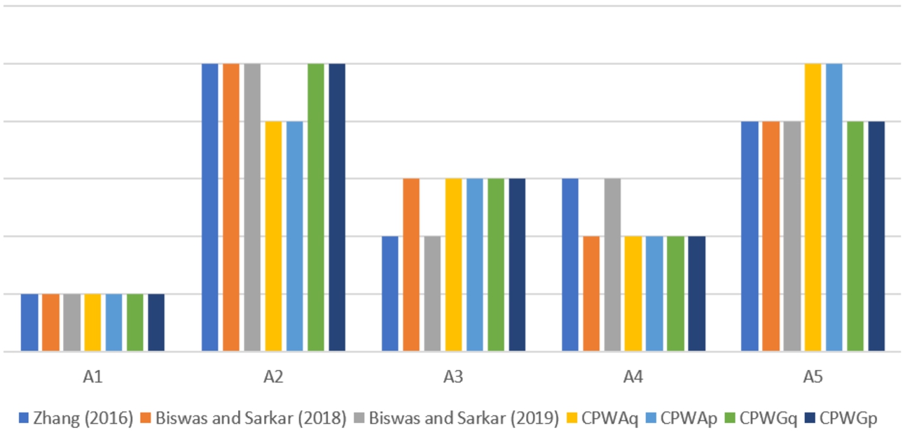
5.4Comparative Analysis

The best alternative remains same with the literature when the aggregation operators CPWGqA and CPWGpA are used. On the other hand, the orders of best and second best alternative interchange when the aggregation operators CPWAqA and CPWApA are used. The worst alternative is totally consistent with the literature. The comparison of the other methods proposed to solve this MCDM problem and the method we propose is shown in Table 8 and illustrated in Fig. 7.

Table 8

The comparison of the other methods and proposed method.

Methods	Ranking order	Best Alternative
Zhang (2016)	A1≺A3≺A4≺A5≺A2	A2
Biswas and Sarkar (2018)	A1≺A4≺A3≺A5≺A2	A2
Biswas and Sarkar (2019)	A1≺A3≺A4≺A5≺A2	A2
Proposed Method (CPWAqA)	A1≺A4≺A3≺A2≺A5	A5
Proposed Method (CPWApA)	A1≺A4≺A3≺A2≺A5	A5
Proposed Method (CPWGqA)	A1≺A4≺A3≺A5≺A2	A2
Proposed Method (CPWGpA)	A1≺A4≺A3≺A5≺A2	A2

Fig. 7

The column chart comparison of other methods and the proposed method.

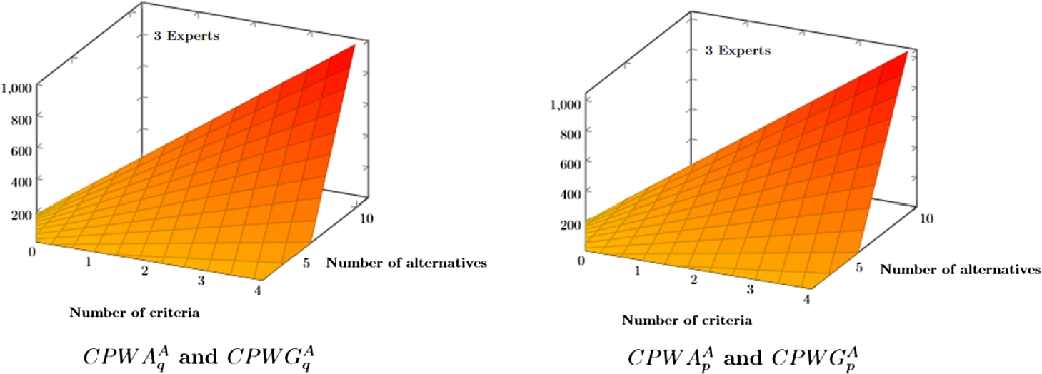
5.5Time Complexity of the Proposed MCDM Method

In this section, we investigate the time complexity of the MCDM method given in Section 5.2. We assume that m experts assign PFVs to create the decision matrix as in the problem solved in Sub-section 5.3. Essentially, the time complexity that depends on the number of times of multiplication, exponential, summation as in Chang (1996) and Junior et al. (2014) is evaluated. Consider a MCDM problem with n alternatives, k criteria and m experts. In Step 2, we need k+2knm operations, in Step 3, we need nk(10m+6) operations, in Step 4, we need n(8k+2) operations if we utilize the aggregation operator CPWAqA, we need n(10k+4) operations if we utilize the aggregation operator CPWApA, we need n(8k+2) operations if we utilize the aggregation operator CPWGqA and we need n(10k+4) operations if we utilize the aggregation operator CPWGpA. In Step 5, we need 23n operations. Therefore, the time complexity is

Comp(k,n;m)=k+2kn(6m+7)+25n

for the aggregation operators CPWAqA and CPWGqA,

Comp(k,n;m)=k+4kn(3m+4)+27n

for the aggregation operators CPWApA and CPWGpA. Obviously, the bi-variate functions gq,gp:[2,∞)→R defined by gmq(x,y)=x+2xy(6m+7)+25y and gmp(x,y)=x+4xy(3m+4)+27y assume global minimum at point (2,2) for any fixed positive integer m. Figure 8 visualizes the change of the time complexity with respect to the change in the numbers of the criteria, the alternatives and the experts for CPWAqA, CPWApA, CPWGqA and CPWGpA.

Fig. 8

Time complexity of the proposed MCDM method.

6Conclusion

The main goal of this paper is to introduce the concept of C-PFS represented by a circle whose radius is r and whose centre consists of a pair with the condition that the sum of the square of the components is less than one. In such a fuzzy set, the membership degree and the non-membership degree are represented by a circle. Thus, a C-PFS is a generalization of both C-IFSs and PFSs. C-PFSs allow decision makers or experts to evaluate objects in a larger and more flexible region compared to both C-IFSs and PFSs. Therefore, the change of membership degree and non-membership degree can be handled to express uncertainty with the help of C-PFSs. In this way, more sensitive decisions can be made. In this paper, a method is developed to transform PFVs to a C-PFV. Also, some fundamental set theoretic operations for C-PFSs are given and some algebraic operations for C-PFVs via continuous Archimedean t-norms and t-conorms are introduced. Then with the help of these algebraic operations some weighted aggregation operators for C-PFVs are presented. Inspired by a cosine similarity measure defined between PFVs, we give a cosine similarity measure based on radius to determine the degree of similarity between C-PFVs. Finally, by utilizing the concepts mentioned above we propose an MCDM method in circular Pythagorean fuzzy environment and we apply the proposed method to an MCDM problem from the literature about selecting the best photovoltaic cell (also known as solar cell). We compare the results of the proposed method with the existing results and calculate the time complexity of the MCDM method. In the future studies, different kind of aggregation operators and similarity measures can be investigated. Also, while transforming PFVs to a C-PFV, other aggregation tool as fuzzy integrals or aggregation operators can be used. Moreover, the proposed method can be used to solve MCDM problems such as classification, pattern recognition, data mining, clustering and medical diagnosis.

Acknowledgements

The authors are grateful to the reviewers for carefully reading the manuscript and for offering many suggestions which resulted in an improved presentation.

References

1	Atanassov, K., Marinov, E. ((2021) ). Four distances for circular intuitionistic fuzzy sets. Mathematics, 9(10): , 1121.
2	Atanassov, K.T. ((1986) ). Intuitionistic fuzzy sets. Fuzzy Sets and Systems, 20: , 87–96.
3	Atanassov, K.T. ((1999) ). Intuitionistic fuzzy sets. In: Intuitionistic Fuzzy Sets. Studies in Fuzziness and Soft Computing, Vol. 35: . Physica, Heidelberg. https://doi.org/10.1007/978-3-7908-1870-3_1.
4	Atanassov, K.T. ((2020) ). Circular intuitionistic fuzzy sets. Journal of Intelligent and Fuzzy Systems, 39(5): , 5981–5986.
5	Becquerel, E. ((1839) ). Mémoire sur les effets électriques produits sous l’influence des rayons solaires. Comptes Rendus, 9: , 561–567.
6	Beliakov, G., Pradera, A., Calvo, T. ((2007) ). Aggregation Functions: A Guide for Practitioners, Vol. 221. Springer, Heidelberg.
7	Beliakov, G., Bustince, H., Goswami, D.P., Mukherjee, U.K., Pal, N.R. ((2011) ). On averaging operators for Atanassov’s intuitionistic fuzzy sets. Information Sciences, 181: , 1116–1124.
8	Biswas, A., Sarkar, B. ((2018) ). Pythagorean fuzzy multicriteria group decision making through similarity measure based on point operators. International Journal of Intelligent Systems, 33(8): , 1731–1744.
9	Biswas, A., Sarkar, B. ((2019) ). Pythagorean fuzzy TOPSIS for multicriteria group decision-making with unknown weight information through entropy measure. International Journal of Intelligent Systems, 34(6): , 1108–1128.
10	Boltürk, E., Kahraman, C. ((2022) ). Interval-valued and circular intuitionistic fuzzy present worth analyses. Informatica, 33(4): , 693–711.
11	Chang, D.Y. ((1996) ). Applications of the extent analysis method on fuzzy AHP. European Journal of Operational Research, 95(3): , 649–655.
12	Garg, H. ((2016) ). A new generalized Pythagorean fuzzy information aggregation using Einstein operations and its application to decision making. International Journal of Intelligent Systems, 31(9): , 886–920.
13	Garg, H., Arora, R. ((2021) ). Generalized Maclaurin symmetric mean aggregation operators based on Archimedean t-norm of the intuitionistic fuzzy soft set information. Artificial Intelligence Review 54: , 3173–3213.
14	Grabisch, M., Marichal, J.L., Mesiar, R., Pap, E. ((2009) ). Aggregation Functions. Cambridge University Press.
15	Junior, F.R.L., Osiro, L., Carpinetti, L.C.R. ((2014) ). A comparison between fuzzy AHP and Fuzzy TOPSIS methods to supplier selection. Applied Soft Computing, 21: , 194–209.
16	Kahraman, C. ((2008) ). Fuzzy Multi-Criteria Decision Making: Theory and Applications with Recent Developments, Vol. 16. Springer Science and Business Media.
17	Kahraman, C., Alkan, N. ((2021) ). Circular intuitionistic fuzzy TOPSIS method with vague membership functions: supplier selection application context. Notes on Intuitionistic Fuzzy Set, 27(1): , 24–52.
18	Kahraman, C., Otay, I. ((2022) ). Extension of VIKOR method using circular intuitionistic fuzzy sets. In: Kahraman, C., Cebi, S., Cevik Onar, S., Oztaysi, B., Tolga, A.C., Sari, I.U. (Eds.), Intelligent and Fuzzy Techniques for Emerging Conditions and Digital Transformation, INFUS 2021, Lecture Notes in Networks and Systems, Vol. 308: . Springer, Cham. https://doi.org/10.1007/978-3-030-85577-2_6.
19	Klement, E.P., Mesiar, R., Pap, E. ((2002) ). Triangular Norms. Kluwer Academic Publishers, Dordrecht.
20	Klement, E.P., Mesiar, R., Pap, E. ((2004) a). Triangular norms. Position paper I: basic analytical and algebraic properties. Fuzzy Sets and Systems, 143: (1), 5–26.
21	Klement, E.P., Mesiar, R., Pap, E. ((2004) b). Triangular norms. Position paper III: continuous t-norms. Fuzzy Sets and Systems, 145: (3), 439–454.
22	Klir, G., Yuan, B. ((1995) ). Fuzzy Sets and Fuzzy Logic: Theory and Applications. Prentice Hall, Upper Saddle River, NJ.
23	Menger, K. ((1942) ). Statistical metrics. Proceedings of the National Academy of Sciences of the United States of America, 28: (12), 535–537.
24	Olgun, M., Ünver, M., Yardımcı, Ş. ((2019) ). Pythagorean fuzzy topological spaces. Complex and Intelligent Systems, 5(2): , 177–183.
25	Olgun, M., Ünver, M., Yardımcı, Ş. ((2021) a). Pythagorean fuzzy points and applications in pattern recognition and Pythagorean fuzzy topologies. Soft Computing, 25(7): , 5225–5232.
26	Olgun, M., Türkarslan, E., Ünver, M., Ye, J. ((2021) b). A cosine similarity measure based on the Choquet integral for intuitionistic fuzzy sets and its applications to pattern recognition. Informatica, 32: (4), 849–864.
27	Peng, X., Yuan, H., Yang, Y. ((2017) ). Pythagorean fuzzy information measures and their applications. International Journal of Intelligent Systems, 32: (10), 991–1029.
28	Schweizer, B., Sklar, A. ((1983) ). Probabilistic Metric Spaces. North-Holland, New York.
29	Socorro García-Cascales, M., Teresa Lamata, M., Miguel Sánchez-Lozano, J. ((2012) ). Evaluation of photovoltaic cells in a multi-criteria decision making process. Annals of Operations Research, 199(1): , 373–391.
30	Verma, R., Sharma, B.D. (2013). Intuitionistic fuzzy Jensen-Rényi divergence: applications to multiple-attribute decision making. Informatica, 37(4).
31	Wan, S., Dong, J. ((2014) ). Multi-attribute group decision making with trapezoidal intuitionistic fuzzy numbers and application to stock selection. Informatica, 25: (4), 663–697.
32	Wei, G., Wei, Y. ((2018) ). Similarity measures of Pythagorean fuzzy sets based on the cosine function and their applications. International Journal of Intelligent Systems, 33: (3), 634–652.
33	Yager, R.R. ((2013) a). Pythagorean fuzzy subsets. In: 2013 Joint IFSA World Congress and NAFIPS Annual Meeting (IFSA/NAFIPS), Edmonton, AB, Canada, 2013, pp. 57–61. https://doi.org/10.1109/IFSA-NAFIPS.2013.6608375.
34	Yager, R.R. ((2013) b). Pythagorean membership grades in multicriteria decision making. IEEE Transactions on Fuzzy Systems, 22(4): , 958–965.
35	Yager, R.R., Abbasov, A.M. ((2013) ). Pythagorean membership grades, complex numbers, and decision making. International Journal of Intelligent Systems, 28: (5), 436–452.
36	Yang, Y., Chin, K.S., Ding, H., Lv, H.X., Li, Y.L. ((2019) ). Pythagorean fuzzy Bonferroni means based on T-norm and its dual T-conorm. International Journal of Intelligent Systems, 34: (6), 1303–1336.
37	Ye, J., Türkarslan, E., Ünver, M., Olgun, M. ((2022) ). Algebraic and Einstein weighted operators of neutrosophic enthalpy values for multi-criteria decision making in neutrosophic multi-valued set settings. Granular Computing, 7: (3), 479–487.
38	Yeni, F.B., Özçelik, G. ((2019) ). Interval-valued Atanassov intuitionistic fuzzy CODAS method for multi criteria group decision making problems. Group Decision and Negotiation, 28: (2), 433–452.
39	Yolcu, A., Smarandache, F., Öztürk, T.Y. ((2021) ). Intuitionistic fuzzy hypersoft sets. Communications Faculty of Sciences University of Ankara Series A1 Mathematics and Statistics, 70: (1), 443–455.
40	Zadeh, L.A. ((1965) ). Fuzzy sets. Information and Control, 8: (3), 338–353.
41	Zeng, S., Cao, C., Deng, Y., Shen, X. ((2018) ). Pythagorean fuzzy information aggregation based on weighted induced operator and its application to R&D projections selection. Informatica, 29: (3), 567–580.
42	Zhang, X. ((2016) ). A novel approach based on similarity measure for Pythagorean fuzzy multiple criteria group decision making. International Journal of Intelligent Systems, 31: (6), 593–611.
43	Zhang, X., Xu, Z. ((2014) ). Extension of TOPSIS to multiple criteria decision making with Pythagorean fuzzy sets. International Journal of Intelligent Systems, 29: (12), 1061–1078.
44	Ünver, M., Olgun, M., Türkarslan, E. ((2022) a). Cosine and cotangent similarity measures based on Choquet integral for Spherical fuzzy sets and applications to pattern recognition. Journal of Computational and Cognitive Engineering, 1: (1), 21–31.
45	Ünver, M., Türkarslan, E., Çelik, N., Olgun, M., Ye, J. ((2022) b). Intuitionistic fuzzy-valued neutrosophic multi-sets and numerical applications to classification. Complex and Intelligent Systems, 8: (2), 1703–1721.