On Order Policies for a Perishable Product in Retail

Hendrix, Eligius M.T.; Pauls-Worm, Karin G.J.; de Jong, Maartje V.

doi:10.15388/23-INFOR520

On Order Policies for a Perishable Product in Retail

Article type: Research Article

Authors: Hendrix, Eligius M.T.^{1; ∗} | Pauls-Worm, Karin G.J.² | de Jong, Maartje V.³

Affiliations: [1] Computer Architecture, Universidad de Málaga, Spain | [2] Operations Research and Logistics, Wageningen University, The Netherlands | [3] Wageningen Economic Research, Wageningen University & Research, The Netherlands

Correspondence: [∗] Corresponding author.

Keywords: perishable, inventory, service level, order policy

DOI: 10.15388/23-INFOR520

Journal: Informatica, vol. 34, no. 2, pp. 271-283, 2023

Received November 2022

Accepted May 2023

Published: 2023

Get PDF

Abstract

We study an inventory control problem of a perishable product with a fixed short shelf life in Dutch retail practice. The demand is non-stationary during the week but stationary over the weeks, with mixed LIFO and FIFO withdrawal. The supermarket uses a service level requirement. A difficulty is that the age-distribution of products in stock is not always known. Hence, the challenge is to derive practical and efficient order policies that deal with situations where this information is either available or lacking. We present the optimal policy in case the age distribution is known, and compare it with benchmarks from literature. Three heuristics have been developed that do not require product age information, to align with the situation in practice. Subsequently, the performance of the heuristics is evaluated using demand patterns from practice. It appears that the so-called STIP heuristic (S for Total estimated Inventory of Perishables) provides the lowest cost and waste levels.

1Introduction

Supermarket managers face a trade-off between risking to lose both revenue and goodwill by not having products available when demand arises on the one hand, and discarding surplus products, due to out-dating, on the other hand (Gruen et al., 2002). Food waste is mainly a result of retailer and consumer behaviour (Parfitt et al., 2010). Food waste occurs in two ways; either in markdowns when products are still saleable but approach the end of their shelf life or appear less attractive, or in garbage when products are no longer (re)saleable, usable or edible. In Europe, the total food loss and waste is 31% of the initial production from which 6.1% occurs during food processing, packaging and distribution (HLPE, 2014). Leberorger and Schneider (2014) report a food loss rate of fruit and vegetables of 4.19% in an Austrian food retail company from September 2011 to August 2012. For dairy products, the food loss rate was 1.14%, and for bread and pastry – 2.84%.

Generally, retailers rather build up more stock than risk a stock-out (Thyberg and Tonjes, 2016). Moreover, availability of fresher items significantly affects consumer choice on where to shop (Wyman, 2013). Furthermore, the demand rate is influenced by product availability and freshness (Sebatjane and Adetunji, 2021). So, there is simply a business incentive for retailers to overstock. This is not without risk. Waste represents a loss of business and a risk for already small margins (Cicatiello et al., 2017). Reducing the annual food waste will result in benefits for companies, consumers and the environment in terms of money, volume, energy and sustainability. Retailers are therefore very keen to implement strategies to reduce food waste. To illustrate this, members of the Consumer Goods Forum promised in 2015 to halve the food they waste by 2025 (The Consumer Goods Forum, 2015). This motivates looking for order policies that may help to reduce food waste and at the same time reduce costs for retailers. Many recent studies, such as (Herbon, 2017) and (Buisman et al., 2019), focus on discounting and adapting prices when the product approaches the expiration date, as a way of waste reduction. However, the competitive strategy of the retailer we study focuses on availability of fresh produce for fixed prices, without discounting, applying strict service level requirements. This relates to waste prevention. In the case of dynamic pricing, profit maximization and waste reduction do not necessarily go along, while in our case cost minimization and waste reduction are equivalent.

The Dutch retailer case studied in this paper enhances a highly perishable product inventory system with a fixed shelf life of three days on delivery at the store, noticeable by its best-before or use-by date. The supermarket is replenished every day which implies the retailer has items of different ages in stock. In many practical retail situations, the checkout system only registers the number of items sold but not their age, see Pantsar (2019). Consequently, the retailer is facing an order decision without knowledge of the age-distribution of the remaining items in stock. The observed total number of items in stock may be different from the inventory status according to the checkout system, due to damaged items and the occurrence of more waste than expected based on supply and demand data of the supermarket. In order to minimize waste, supermarkets prefer and stimulate customers to pick the oldest items first (FIFO, First In First Out), by putting those items in front on the shelf. However, practitioners in Dutch retail estimate that about 40% of the customers search for the freshest items and pick according to LIFO (Last In First Out).

Competition among supermarkets stimulates the aim to have fresh produce available. The product availability of a supermarket can be observed by the number of days the items are in-stock (not out-of-stock) in a supermarket. To monitor and ensure product availability, supermarkets generally set a target service level. In case of lost demand and periodic review of inventory levels, a so-called α-service level is most suitable. On the other hand, a supermarket aims at limiting product waste. By appropriate order policies, waste prevention can be improved.

Literature discusses several approaches in case the cash registering enhances the age of the sold products. This means that the age of items that remain in stock is known. In this paper, we will derive the optimal policy for this situation. However, we found that in retail practice the age is often not registered. This means that only the total number of items in stock is known after the products that expired their shelf life have been thrown out. Therefore, our aim is to derive practical heuristics in case the age distribution of the stock is unknown to approximate the situation in practice more accurately.

This paper is organised as follows. Section 2 describes the retail situation and a stochastic dynamic model of the situation. Section 3 discusses various approaches to determine the order quantity and Section 4 shows the results of numerical experiments based on practical data for the approaches. A discussion of findings and conclusions can be found in Section 5.

2Model of the Retail Situation Inventory Control

To be able to model the stochastic dynamics for this problem, it is necessary to first identify the underlying characteristics of the practical situation. These characteristics are discussed in Section 2.1 and the model in Section 2.2.

Table 1

Table with used symbols.

Indices
t	Day of the week, t=1,…,7
b	Age of item in stock, b=1,…,M, M=3
L	Lead time, L=1
Data
c	Purchasing cost per item
μt	Expected demand day t
dt	Random demand day t, Poisson distributed
α	Service level requirement as probability
λ	Probability a client selects according to LIFO
St	Order up-to level day t
Variables
Qt	Order quantity day t
Ibt	Number of items in stock of age b at the end of day t

2.1Description of the Retail Situation

In this study, a period t in the model is a day at the store, from opening until closing time. In the retail practice of perishable products, mostly the order quantity Qt of today is delivered the next day, so the lead time is L=1 day. The used symbols are presented in Table 1. In the model the sequence of events is as follows:

1. Store opening;
2. Delivery of quantity Qt−1;
3. Ordering of quantity Qt;
4. Demand during the day from a mixed LIFO and FIFO withdrawal, ageing of remaining items in stock and disposal of wasted items, at store closure.

At the moment of the order decision, the previous order has arrived, so there is no outstanding order. The order quantity is based on the on-hand inventory and the expected demand during the replenishment cycle. At the end of day t, the inventory level Ibt is realized for items of all ages b. So, items from quantity Qt−1 delivered on day t have age b=1 at the end of day t. Items with an age reaching the shelf life b=M, are waste and removed from the shelf at the end of the day. In case of waste, the purchasing cost is lost. The time horizon T is 7 days with t=1 being Monday. Inventory at the end of Sunday (T=7) transfers to Monday morning.

The demand is independently Poisson distributed with expectation μt for day t. When demand is higher than the inventory level, sales are lost and the inventory level will be zero. Moreover, we consider a mixed LIFO-FIFO withdrawal, where the number of customers buying LIFO is binomially distributed.

2.2Stochastic Model

The general reorder decision problem can be formulated as a stochastic optimization model that minimizes purchasing cost and fulfils the service level constraint. For this specific model, minimization of cost and minimization of waste coincide.

(1)

min{E(TC):=∑t=1TE(cQt)}.

Let x+:=max{x,0}. The total inventory balance for all ages is given by

(2)

∑b=1MIbt=(∑b=1M−1Ib,t−1+Qt−1−dt)+,

where t−1=0 corresponds to T=7. Period t starts with the inventory levels at the end of period t−1 of ages b=1,…,M−1. Items of age M are waste. The starting inventory is added to the delivered quantity Qt−1 and demand in period t is subtracted to give the end inventory. The service level requirement is put on the probability that sufficient material is available to fulfil demand:

(3)

P(dt⩽∑b=1M−1Ib,t−1+Qt−1)⩾α.

This means that we consider a minimal service level constraint as studied by Chen and Krass (2001), where for every day, on average, the service level has to be met.

The company we cooperated with in this study viewed demand dt for this type of fresh products as Poisson distributed. A part of the customers pick the freshest items first. The distribution of demand into LIFO and FIFO follows a binomial distribution B(dt,λ), with a fraction 0⩽λ⩽1 of customers that choose the items according to LIFO. This means that the LIFO inventory dynamics is followed for LIFO demand binomially drawn from B(dt,λ) and the rest of the customers follow the FIFO dynamics, where demand is fulfilled first by the oldest items before the fresher items. LIFO dynamics is modelled as

(4)

I1t=(Qt−1−dt)+,t=1,…,T

and

(5)

Ibt=(Ib−1,t−1−(dt−Qt−1−∑j=1b−2Ij,t−1)+)+,t=1,…,T,b=2,…,M.

In the FIFO dynamics, first the older items are picked:

(6)

I1t=Qt−1−(dt−∑b=1M−1Ib,t−1)+,t=1,…,T

and

(7)

Ibt=(Ib−1,t−1−(dt−∑j=bM−1Ij,t−1)+)+,t=1,…,T,b=2,…,M.

The model should keep track of the end of the week balance, where

(8)

Ib0=IbTandQ0=QT.

Moreover, order quantities and inventory cannot be negative:

(9)

Qt⩾0,t=1,…,T,

(10)

Ibt⩾0,t=1,…,T,b=1,…,M.

3Order Policies

First of all, we have to distinguish the situation that the age of the products in stock is known versus a practical situation where this is not the case. In the first case, the order quantity Qt as a policy is a function of the vector (Qt−1,I1,t−1,I2,t−1,…,IM−1,t−1). When the distribution is not known, the order quantity is a function of the total available inventory Qt−1+∑b=1M−1Ib,t−1. A specific case of the latter is the so-called base-stock policy (BSP), where an order-up-to level S determines the order quantity Q. The current situation asks for a day dependent order-up-to level St for each day t of the week. The order quantity in terms of an order-up-to policy is determined by

(11)

Qt=(St−Qt−1−∑b=1M−1Ib,t−1)+.

Given a required α-service level, the value St for which the in-stock probability is α is a value St∈{0,1,2,3,…}. Standard textbooks like Chopra and Meindl (2016) cover the derivation of the order-up-to level in a periodic review system taking demand during lead time L and the replenishment cycle into account. The values for S can easily be derived using an Excel or Matlab search routine. In our case, we should determine the minimum value St for which

P(dt+dt+1⩽St)⩾α.

Specifically for the Poisson distribution, this is a value St for which

(12)

P(dt+dt+1⩽St)=eμt+μt+1∑j=0St(μt+μt+1)jj!⩾α.

We will discuss two approaches from literature for the known age distribution in Section 3.1, derive the optimal order quantity in Section 3.2 and deal with the practical situation of not having this information in Section 3.3.

3.1EWA, EWA_ss Heuristics if Oldest Items in Stock are Known

Broekmeulen and Van Donselaar (2009) proposed the so-called Estimated Withdrawal and Ageing (EWA) heuristic, where knowledge of the number of oldest items, which is going to expire during lead time, is known as part of the total inventory. Notice that the lead time is L=1. So in that case, the number of items to expire during lead time is IM−1,t−1. The order quantity is determined by an order-up-to level containing a safety stock, which is corrected for expected waste. Broekmeulen and Van Donselaar (2009) used a fixed safety stock, optimized by simulation. Kiil et al. (2018) determine the safety stock using the standard deviation of forecast errors during lead time and replenishment cycle times a safety factor. Their modified EWA_ss policy uses a smaller buffer stock consisting of the maximum of either the safety stock, or the expected waste. In our implementation, we calculate the safety stock SS in the order-up-to level by

(13)

SSt=St−μt−μt+1.

3.2The Optimal Order Quantity Q∗, if Oldest Items in Stock are Known

Due to the lead time of one day, the optimal order quantity Q∗ can be determined if the number IM−1,t−1 of oldest items in stock at the beginning of the day is known. This means that we can derive a table Q∗(Qt−1+∑b=1M−2Ib,t−1,IM−1,t−1) of optimal order quantities. For the ease of notation, consider the fresh inventory X=Qt−1+∑b=1M−2Ib,t−1 and old inventory Z=IM−1,t−1. The optimal order quantity Q∗(X,Z,t) follows from minimizing order quantity Qt, such that the leftover x of the amount in stock at the end of the day plus the ordered quantity Qt fulfils the demand dt+1 with a required service level α:

(14)

∑x=0XPx(x|X,Z,t)×P(dt+1⩽x+Qt)⩾α.

To find this quantity requires deriving the probability function of the conditional loss function

(15)

Px(x|X,Z,t)=P(∑b=1M−1Ibt=x|X,Z,t).

This is not straightforward, as one not only has to take the probability distribution of dt into account, but also the binomial distribution of LIFO demand. Consider a realization D of demand dt and y the LIFO demand. The boundary of the probability mass function of the loss is the probability that there is no left-over

(16)

Px(0|X,Z,t)=P(dt⩾X+Z)+∑D=XX+Z−1∑y=XDDyλy(1−λ)(D−y)P(dt=D).

The probability mass for obtaining a left-over of 1⩽x⩽X is

(17)

Px(x|X,Z,t)=P(y=X−x)=∑D=X−xX+Z−xDX−xλ(X−x)(1−λ)(D−X+x)P(dt=D).

A practical way to derive the values of the probability distribution of x is to enumerate all events of demand realizations dt=0,…,X+Y−1 and of the binomial event y of the LIFO demand with their probability of occurrence. Then one accumulates the probability on the event on the outcome x. After generating the corresponding probability distribution and minimizing Qt in (14), one obtains the optimal daily ordering table Q∗(X,Z,t) for the case that the retailer not only knows the total inventory level X+Z, but also how many items Z=IM−1,t−1 expire at the end of the day.

3.3Heuristic Policies if the Age Information is Unknown

We developed three heuristics for the order quantity based on the knowledge of the total inventory for the case that the age of the items in stock is not known.

• An easy way to deal with lack of knowledge of the oldest items in stock is to simulate the system using the table of Q∗ and derive the corresponding average rounded value for order-up-to levels St. Basically, we simulate the system with knowledge of the oldest items in stock and measure the realizations Xt and Zt of the inventory system and average observations of the revealed order-up-to level St=Qt+Xt+Zt using Qt=Q∗(X,Z,t) for each day t of the week. The computational procedure requires simulating the optimal Q∗ with the known age distribution only once. We call this heuristic S for Total estimated Inventory of Perishables, STIP.
• In the Expected Waste heuristic SEW, the order quantity Qt is determined by (11) using order-up-to level St from (12) corrected by an expected waste estimate considering a mixed expected LIFO-FIFO demand and the inventory dynamics. If a stock-out occurs, i.e. the supermarket is out of stock, the policy takes as order quantity Qt=St. This means that the computation of the order quantity is based on predefined values following from probability theory.
• In the S_Augmented heuristic, we also use order-up-to level policy (12). However, the order-up-to levels St have been defined by simulating the system and incrementing the values if service levels are not reached. The actual order quantity Qt is determined by (11), but in case a stock-out occurs, the policy takes as order quantity Qt=St. In a simulation-optimization approach, if the average service level (SL) in a simulation is below the target on day t, the order-up-to level of of day t−1 is incremented by one unit. The new order-up-to levels St are input in a new simulation run, until for all days the target SL is met. The result is a vector (S1,S2,…,S7) of order-up-to levels that meets the SL requirement.

4Numerical Evaluation

We evaluate the described order policies. The design of experiments is described in Section 4.1, followed by the obtained results in Section 4.2. In Section 4.3 we discuss some computational aspects.

4.1Design of Experiments

All approaches are evaluated in a rolling horizon simulation of 10,000 weeks using pseudo random samples from the Poisson – and the binomial distribution. The expected demand μt varies during the week. A base demand pattern is taken from observed data in a practical retail case regarding iceberg lettuce. To evaluate the effect of larger numbers, a double base pattern has been designed. A pattern with higher peaks on Wednesday and Saturday provides more challenge to fulfil the service level and has therefore been included. The target service level is taken as α=90%. The evaluated three demand patterns are depicted in Fig. 1. Table 2 provides the exact numbers of the expected values in order to be able to repeat the experiments.

Fig. 1

Evaluated expected demand patterns during the week. Day 1 corresponds to Monday.

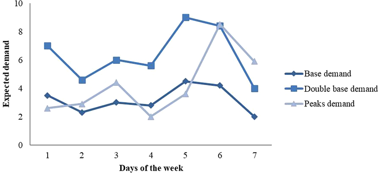
Table 2

Expected Poisson demand.

	Monday	Tuesday	Wednesday	Thursday	Friday	Saturday	Sunday
Period t	1	2	3	4	5	6	7
Base μt	3.5	2.3	3.0	2.8	4.5	4.2	2.0
Double base μt	7.0	4.6	6.0	5.6	9.0	8.4	4.0
Peaks μt	2.6	2.9	4.4	2.0	3.6	8.5	5.9

The variable purchasing cost is c=1 per unit. As a result, the average total cost per week is equal to the average order quantity per week. The practitioners in retail we consulted, estimate a LIFO fraction of about 0.4 to be realistic. For the base demand pattern, we vary the fraction of LIFO demand λ∈{0,0.4,0.6} for all schedules. To show the effect of partly LIFO demand on the order policies and the average amount of waste, also the situation of only FIFO withdrawal and a LIFO fraction of 0.6 are investigated for the base demand pattern. The other demand patterns are evaluated for a LIFO fraction of λ=0.4, for all schedules.

4.2Results

Table 3 summarizes the results for the base demand pattern for all described approaches. It shows the average total cost (avgTC) and the average total waste (avgTW) per week. To observe the feasibility of the policy with respect to the minimal service level (SL) constraint, the attained SL is measured for each day. We provide the minimum of these values over the days of the week (minSL) in the table. The policies using information about the oldest items in stock are supposed to do better than the heuristic policies that do not use this information. As expected, one can observe that the costs and the number of wasted items increase when the fraction of LIFO demand increases.

Table 3

Results for base demand with LIFO fractions λ∈{0,0.4,0.6}. Average total cost, total waste and minimum service level in the week.

Knowledge oldest items in stock
Policy	EWA			EWA_ss			Q∗

λ	avgTC	avgTW	minSL	avgTC	avgTW	minSL	avgTC	avgTW	minSL
0	23.19	1.59	0.92	23.05	1.53	0.93	22.65	1.20	0.92
0.4	24.87	3.25	0.93	24.21	2.86	0.91	24.05	2.63	0.93
0.6	26.22	4.55	0.94	24.94	3.69	0.90	25.05	3.63	0.92

Age items in stock unknown
Policy	STIP			SEW			S_augmented

λ	avgTC	avgTW	minSL	avgTC	avgTW	minSL	avgTC	avgTW	minSL
0	22.77	1.34	0.91	23.14	1.56	0.93	24.00	2.66	0.90
0.4	23.91	2.68	0.91	24.56	3.07	0.92	25.00	3.69	0.90
0.6	24.57	3.47	0.89	25.59	4.16	0.91	26.00	4.60	0.91

Table 4 compares all approaches for the three demand patterns with a LIFO fraction of λ=0.4. From the measured performance indicators in Tables 3 and 4, it is surprising to observe that the policies STIP, SEW and S_augmented, which do not require age information, perform even better than the EWA policy. In this case, EWA_ss has also lower costs and waste than the EWA approach, validating the claim of Kiil et al. (2018). However, in case of the double base demand, the EWA approach outperforms the EWA_ss approach, which does not consistently meet the service level constraint due to a lowest attained SL of 0.88. Q∗ gives the optimal order policy when age information is available. One might expect a reached SL of 0.90 in this approach, but the measured SL is higher due to the small numbers of discrete demand. However, the over achievement may also be related to the conditional character of the order policy as described by Pauls-Worm and Hendrix (2015).

The SEW approach quickly generates easy-to-calculate order quantities with feasible results. The only exception occurs for the peak demand pattern where a minimum average SL of 0.89 is reached for one of the days. The STIP approach, which corresponds to lowest costs and waste and reasonable service levels, fails to reach the target SL of 90% for the double base demand and peaks demand patterns, reaching an average SL of 0.89 for one of the days, which is still close to the target level.

Table 4

Results for 3 demand patterns with LIFO fraction λ=0.4. Average total cost, total waste and minimum service level in the week.

Pattern policy	Base demand			Double base demand			Peaks demand
	avgTC	avgTW	minSL	avgTC	avgTW	minSL	avgTC	avgTW	minSL
	EWA	24.87	3.25	0.93	46.01	2.49	0.93	33.04	3.92	0.92
EWA_ss	24.21	2.86	0.91	45.63	2.33	0.88	32.24	3.39	0.90
Q∗	24.05	2.63	0.93	45.36	2.06	0.92	32.15	3.25	0.92
STIP	23.91	2.86	0.91	45.41	2.19	0.89	32.05	3.32	0.89
SEW	24.56	3.07	0.92	45.71	2.35	0.90	32.53	3.60	0.89
S_augmented	24.31	2.95	0.91	45.72	2.39	0.91	32.49	3.63	0.92

4.3Computational Aspects

The evaluated approaches include four new approaches to determine order policies. The existing policies – EWA Broekmeulen and Van Donselaar (2009) and EWA_ss Kiil et al. (2018) policy – require knowledge of the oldest items in stock. As a benchmark, we evaluated the newly derived optimal quantity Q∗ policy.

The EWA, EWA_ss and SEW approaches offer easy and fast calculation rules to determine the order quantity. Like the determination of table Q∗, they require computation based on probability theory. Basically, the complexity would increase linearly with the considered horizon T. However, in the practical retail setting, the stationary behaviour captures one week. The STIP approach follows from simulating the Q∗ policy only once. However, the complexity of the simulation-optimization S_augmented approach depends also on the number of iterations of increments to reach a solution which is feasible in terms of service level. Computing time is hard to compare among the implemented methods, because different software and processors were used. The computational speed also depends on the way of programming.

For the investigated experiments, determination of Q∗ requires for all experiments about 7.5 s. The S_augmented heuristic needs 4.5 s to 9.0 s. These experiments were performed in Matlab, on an Intel Core i7-4770 CPU, 3.40 GHz desktop processor.

5Conclusion

The research question of this paper deals with the development and investigation of order policies for a Dutch retail situation with a service level requirement where the age-distribution of the inventory may be known or unknown. We investigated a retail situation where a product has a fixed shelf life of three days upon delivery, demand is non-stationary during the week, but stationary over the weeks, with a mixed LIFO-FIFO depletion and a lead time of one day. For all patterns of expected demand, the policy that provides the minimum amount of waste coincides with the one that minimizes expected cost. This is a logical consequence in absence of the disposal cost or salvage value and not focusing on a profit margin.

In case of having information of the oldest items in stock that are going to expire when not sold, two heuristic approaches can be found in literature, EWA and EWA_ss. In this paper, we derive the optimal order quantity as function of the state of inventory where the LIFO-FIFO demand is described by a binomial distribution.

In case of not having age information, the developed S_augmented heuristic performs best, it always meets the service level requirement and has lower costs than the SEW approach and the benchmark EWA approach. The costs and waste in case of partly LIFO demand are slightly higher than those of the EWA_ss benchmark. However, the benchmark approaches from literature take the age-distribution of the inventory into account. The STIP approach provides the lowest costs and lowest waste, but in some cases it does not reach the target service level of 0.90, providing an attained SL of 0.89 on one day of the week.

Future research deals with the derivation of heuristics for the practical cases where the shop cannot be delivered on all days of the week. This means that a varying replenishment cycle length has to be taken into account.

References

1	Broekmeulen, R.A., Van Donselaar, K.H. ((2009) ). A heuristic to manage perishable inventory with batch ordering, positive lead-times, and time-varying demand. Computers & Operations Research, 36: (11), 3013–3018.
2	Buisman, M.E., Haijema, R., Bloemhof-Ruwaard, J.M. ((2019) ). Discounting and dynamic shelf life to reduce fresh food waste at retailers. International Journal of Production Economics, 209: , 274–284.
3	Chen, F.Y., Krass, D. ((2001) ). Inventory models with minimal service level constraints. European Journal of Operational Research, 134: , 120–140.
4	Chopra, S., Meindl, P. ((2016) ). Supply Chain Management: Strategy, Planning, and Operation. Pearson Education, Michigan, pp. 528.
5	Cicatiello, C., Franco, S., Pancino, B., Blasi, E., Falasconi, L. ((2017) ). The dark side of retail food waste: evidences from in-store data. Resources, Conservation and Recycling, 125: , 273–281.
6	Gruen, T.W., Corsten, D.S., Bharadwaj, S. ((2002) ). Retail Out-of-Stocks: A Worldwide Examination of Extent, Causes and Consumer Responses. Grocery Manufacturers of America, Washington, DC.
7	Herbon, A. ((2017) ). Should retailers hold a perishable product having different ages? The case of a homogeneous market and multiplicative demand model. International Journal of Production Economics, 193: , 479–490.
8	Kiil, K., Hvolby, H.-H., Fraser, K., Dreyer, H., Strandhagen, J.O. ((2018) ). Automatic replenishment of perishables in grocery retailing: the value of utilizing remaining shelf life information. British Food Journal, 120: (9), 2033–2046.
9	Leberorger, S., Schneider, F. ((2014) ). Food loss rates at the food retail, influencing factors and reasons as a basis for waste prevention measures. Waste Management, 34: , 1911–1919.
10	Pantsar, H. (2019). Estimation of Daily Batch Balances of Perishable Products in Retail. Master’s thesis, Aalto University, Finland.
11	Parfitt, J., Barthel, M., Macnaughton, S. ((2010) ). Food waste within food supply chains: quantification and potential for change to 2050. Philosophical Transactions of the Royal Society B: Biological Sciences, 365: (1554), 3065–3081.
12	Pauls-Worm, K.G., Hendrix, E.M. ((2015) ). SDP in inventory control: non-stationary demand and service level constraints. In: International Conference on Computational Science and Its Applications, LNCS, Vol. 9156. Springer, pp. 397–412.
13	Sebatjane, M., Adetunji, O. ((2021) ). Optimal lot-sizing and shipment decisions in a three-echelon supply chain for growing items with inventory level- and expiration date-dependent demand. Applied Mathematical Modelling, 90: , 1204–1225.
14	The Consumer Goods Forum (2015). Consumer Goods Industry Commits to Food Waste Reduction.
15	Thyberg, K.L., Tonjes, D.J. ((2016) ). Drivers of food waste and their implications for sustainable policy development. Resources, Conservation and Recycling, 106: , 110–123.
16	Wyman, O. (2013). Getting fresh: lessons from the global leaders in fresh food. http://www.oliverwyman.com/content/dam/oliver-wyman/europe/germany/de/insights/publications/2015/jan/OW_POV_Getting%20Fresh.pdf.