
Multi-Querying: A Subsequence Matching Approach to Support Multiple Queries
Abstract
The widespread use of sensors has resulted in an unprecedented amount of time series data. Time series mining has experienced a particular surge of interest, among which, subsequence matching is one of the most primary problem that serves as a foundation for many time series data mining techniques, such as anomaly detection and classification. In literature there exist many works to study this problem. However, in many real applications, it is uneasy for users to accurately and clearly elaborate the query intuition with a single query sequence. Consequently, in this paper, we address this issue by allowing users to submit a small query set, instead of a single query. The multiple queries can embody the query intuition better. In particular, we first propose a novel probability-based representation of the query set. A common segmentation is generated which can approximate the queries well, in which each segment is described by some features. For each feature, the corresponding values of multiple queries are represented as a Gaussian distribution. Then, based on the representation, we design a novel distance function to measure the similarity of one subsequence to the multiple queries. Also, we propose a breadth-first search strategy to find out similar subsequences. We have conducted extensive experiments on both synthetic and real datasets, and the results verify the superiority of our approach.
1Introduction
In recent years, the plummet in the cost of sensors and storage devices has resulted in massive time series data being captured and has substantially driven the need for the analysis of time series data. Among various analysis and applications, the problem of subsequence matching is of primordial importance, which serves as the foundation for many other data mining techniques, such as anomaly detection (Boniol and Palpanas, 2020; Boniol et al., 2020; Wang et al., 2022), and classification (Wang et al., 2018; Abanda et al., 2019; Iwana and Uchida, 2020; Boniol et al., 2022).
Specifically, given a long time series X, for any query series Q, the subsequence matching problem finds the K number of subsequences from X most similar to Q (top-K query), or finds subsequences whose distance falls within the threshold ε (range query). In the last two decades, plenty of works have been proposed for this problem. Most existing works find results based on the strict distance, like Euclidean distance and Dynamic Time Warping. Among them are scanning-based approaches (Li et al., 2017; Rakthanmanon et al., 2012) and index-based ones (Linardi and Palpanas, 2018; Wu et al., 2019).
Another type of works define the query in a more flexible way. Query-by-Sketch (Muthumanickam et al., 2016) and SpADe (Chen et al., 2007) approximate the query with a sequence of line segments, and find subsequences that can be approximated in a similar way.
Nevertheless, in many real applications, users are unable to accurately and clearly elaborate the query intuition with a single query sequence. Specifically, users may have different strictness requirements for different parts of the query. We illustrate it with the following two examples.
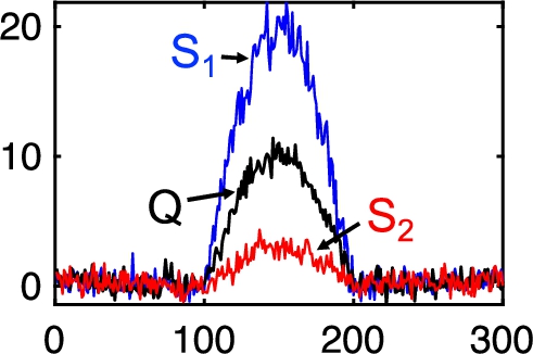
Case study 1. In the field of wind power generation, Extreme Operating Gust (EOG) (Hu et al., 2018) is a typical gust pattern which is a phenomenon of dramatic changes of wind speed in a short period. Early detection of EOG can prevent the damage to the turbine. A typical pattern of EOG, as Q and
Fig. 1
EOG pattern.
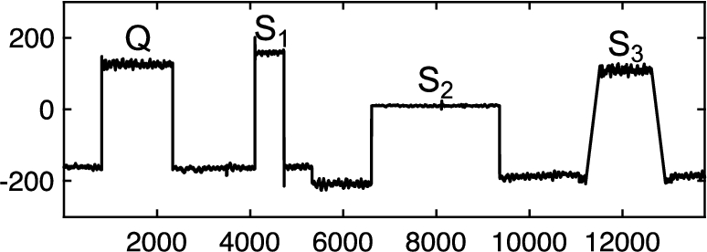
Case study 2. During the high-speed train’s work time, the sensor will continuously collect vibration data for monitoring. When the train passes by some source of interference, the value of sensors will increase sharply, and return to a normal value after some time, as Q,
Fig. 2
Signal interference pattern.
The above examples clearly demonstrate the limitation of the single query mechanism. Although a single query can express the shape the user is interested with, it is not enough to express the extent of time shifting and amplitude scaling, as well as the error range.
To solve this problem, in this paper, we propose a multiple query approach. Compared to a single query, submitting a small number of queries together can express the query intuition more accurately. Consider the example in Fig. 2: if users take Q,
We first propose a probability-based representation of the multiple queries. Then, we design a novel distance function to measure the similarity of one subsequence to the multiple queries. In the end, a breadth-first search algorithm is proposed to find out the desired subsequences. To the best of our knowledge, this is the first work to study how to express the query intuition.
Our contributions can be summarized as follows:
• We analyse the problem of expressing the query intuition, and propose a multi-query mechanism to solve this problem.
• We present a probability-based representation of the multiple queries, as well as the corresponding distance between it and any subsequence.
• We present a breadth-first search algorithm to efficiently search for similar subsequences.
• We conduct extensive experiments on both synthetic and real datasets to verify the effectiveness and efficiency of our approach.
The rest of the paper is organized as follows. The related works are reviewed in Section 2. Section 3 introduces definitions and notations. In Section 4 and 5, we introduce our approach in detail. Section 6 presents an experimental study of our approach using synthetic and real datasets, and we offer conclusions in Section 7.
2Related Work
In last two decades, the problem of subsequence matching has been extensively studied. Existing approaches can be classified into two groups:
Fixed Length Queries: Traditionally, to find out similar subsequences, two representative distance measures are adopted, Euclidean distance (ED) and Dynamic Time Warping (DTW). ED computes the similarity by a one-to-one mapping while DTW allows disalignment and thus supports time shifting. UCR Suite (Rakthanmanon et al., 2012) is a well-known approach that supports both ED and DTW for subsequence matching and proposes cascading lower bounds for DTW to accelerate search speed. FAST (Li et al., 2017) is based on UCR Suite, and further proposes some lower bounds for the sake of efficiency. Both UCR Suite and FAST have to scan the whole time series to conduct distance computation. EBMS (Papapetrou et al., 2011), however, reduces the subsequence matching problem to the vector matching problem, and identifies the candidates of matches by the search of nearest neighbours in the vector space. Also, some index-based approaches have been proposed for similarity search. Most of them build indexes based on summarizations of the data series (e.g. Piecewise Aggregate Approximation (PAA) (Keogh et al., 2001), or Symbolic Aggregate approXimation (SAX) (Shieh and Keogh, 2008)). Coconut (Kondylakis et al., 2018) overcomes the limitation that existing summarizations cannot be sorted while keeping similar data series close to each other and proposes to organize data series based on a z-order curve. To further reduce the index creation time, adaptive indexing techniques have been proposed to iteratively refine the initial coarse index, such as ADS (Zoumpatianos et al., 2016).
Variable Length Queries: For variable length queries, SpADe (Chen et al., 2007) proposes a continuous distance calculation approach, which is not sensitive to shifting and scaling in both temporal and amplitude dimensions. It scans data series to get local patterns, and dynamically finds the shortest path among all local patterns to be the distance between two sequences. Query-by-Sketch (Muthumanickam et al., 2016) proposes an interactive approach to explore user-sketched patterns. It extracts shape grammar, a combination of basic elementary shapes, from the sketched series, and then applies a symbolic approximation based on regular expressions. To better satisfy the user, Eravci and Ferhatosmanoglu (2013) attempts to improve the search results by incorporating diversity in the results for relevance feedback. Relatively speaking, indexing for variable length queries is more intractable.
In summary, up to now, no existing work has attempted to express the query intuition via the multi-query mechanism.
3Preliminaries
In this section, we begin by introducing all the necessary definitions and notations, followed by a formal problem statement.
3.1Definition
In this work, we are dealing with time series. A time series
Given a time series X, a query sequence Q, and a distance function D, the problem of subsequence matching is to find out the top-K subsequences from X, denoted as
The two representative distance measures are Euclidean Distance (ED) and Dynamic Time Warping (DTW). Formally, given two length-L sequences, S and
Definition 1.
Euclidean Distance:
Definition 2.
Dynamic Time Warping:
In this paper, instead of processing one single query, we attempt to find out subsequences similar to multiple queries. That is, given a set of queries,
Since each query sequence varies in length, we do not impose a constraint on the length of subsequences in
4Query Representation and Distance Definition
In this section, we first present the probability-based representation of the query set, and then propose a distance definition based on the representation.
4.1Query Representation
In this paper, instead of processing the queries in
In many real world applications, the meaningful query sequence can be approximately represented as a sequence of line segments. Recall the EOG pattern in Fig. 1. The query sequence Q can be approximated with 4 line segments. These line segments capture the most representative characteristics in Q.
In response, we propose a two-step approach to represent the bundle of queries together. In the first step, we represent each single query
4.1.1Step One: Represent Each Single Query
In step one, we perform a traditional segmentation. We use a bottom-up approach to convert the query
For each line segment
4.1.2Step Two: Represent Multiple Queries
After obtaining
Specifically, given query set
Formally, we denote the representation of
(1)
Now we introduce our approach to generate
4.2Distance Definition
Given the fact that the query representation consists of
Formally, to define the distance between subsequence S and the query representation
(2)
(3)
(4)
5Query Processing Approach
In this section, we introduce the search process. Obviously, it is exhaustive to find out the best segmentation of all subsequences in the time series X. In response, we divide the search process into two phases:
1. Candidate generation. Given the submitted query set
2. Post-processing. All subsequences in
5.1BFS-Based Search Process
We first introduce our search strategy to generate the candidate set
In the second round, we obtain candidate set
After m rounds, we obtain the candidate set
5.2Candidate Generation
Now we introduce our approach to generate possible candidates in each round.
In the first round, we enumerate all subsequences
(5)
In the j-th round (
5.3Post-Processing
Note that the subsequences in
The objective of the segmentation is to minimize the distance between
(6)
Afterwards, we simply sort the remaining subsequences in
5.4Optimization
In this section, we propose two optimization strategies to further accelerate the search process.
5.4.1Basic Aggregates Based Linear Representation Computation
In the search process, for each candidate, we adopt linear regression to find out the best line segment
However, to process extremely long sequences, the storage overheads are unaffordable. As a consequence, we propose to split the time series into several blocks and conduct subsequence matching within each block sequentially and summarize the results in the end. Obviously, this approach reduces memory consumption while being accurate and efficient.
5.4.2Adjusting the Searching Order
Up to now, we have generated the candidates segment-by-segment sequentially. However, different standard deviation of the feature values of different segments in
5.5Complexity Analysis
The overall process of our approach can be divided into two phases: query representation and query processing.
Before the two phases, we have to scan the whole time series X once to store the basic aggregates. Its time cost is
Then, in the first phase, we scan all the queries and perform traditional piecewise linear approximations. Thanks to the basic aggregates, the time cost of conducting linear regression is negligible. This phase is then
In the second phase, we first assume
Since
6Experiments
In this section, we conduct extensive experiments to verify the effectiveness and efficiency of our approach. All experiments are run on a PC with Intel Core i7-7700K CPU (8 cores @ 4.2 GHz) and 16 GB RAM.
6.1Datasets
6.1.1Synthetic Datasets
We generate the synthetic sequence as follows. First, we generate a long random walk sequence T. Then we embed in T some meaningful pattern instances, in which some are taken as queries, and others as target results.
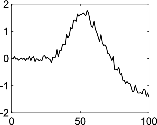
Fig. 3
Two fundamental patterns.
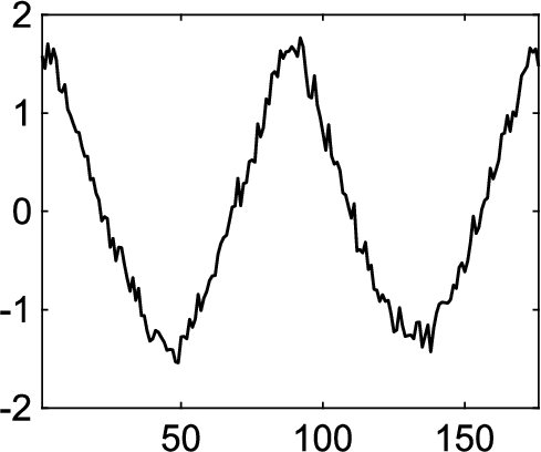 |
| (a) W-wave |
 |
| (b) Backward wave |
We generate two types of patterns, W-wave from the Adiac dataset in UCR archive (Dau et al., 2019), and backward wave, common in stock series. For each pattern, we first generate a seed instance and add some noise following a Gaussian distribution
∙ Length: It is obvious that the W-wave in Fig. 3(a) can be split into four segments. For the middle two segments, we change the segment length with a scaling factor λ by inserting or deleting some data points. In other words, for a length-l segment, the length of the new segment is
∙ Amplitude: Similar to the case of length scaling, we increase or decrease the amplitude of the middle two segments in the W-wave. We still use a factor λ to control the extent. Specifically, every value in new segment changes to
∙ Shape: For the backward wave shown in Fig. 3(b), we change the global shape of the pattern by modifying the last two segments on both length and amplitude. To be more specific, we change the segment length from l to
Table 1
Influence of variations.
| l | θ | v | ε | |
| Length | √ | √ | ||
| Amplitude | √ | √ | √ | |
| Shape | √ | √ | √ |
For each type of variation, we test our approach under different extents. Take the length variation as an example. To generate a dataset, we first set a parameter r, which determines the length variation range. Specifically, given r, we can only set the length scaling factor λ within the range
For each variation, given the fixed r, we pick out 50 values from the range
Table 2
A summary of the synthetic datasets.
| Dataset | Pattern | Variation | Length |
| 1 | W-wave | Length | 0.7 million |
| 2 | W-wave | Amplitude | 0.7 million |
| 3 | Backward wave | Shape | 0.4 million |
6.1.2Real Datasets
The real dataset is the train monitoring dataset, which is the time series collected by the vibration sensor. Its total length is 15 million. There exist more than 100 interference subsequences that vary in length and amplitude. The length of these subsequences is within the range of 200 to 2500. Consequently, we maintain a query set of size 15 whose lengths almost distribute uniformly between 200 and 2500. The rest ones are leaved as the target results.
6.2Counterpart Approaches
Note that it is difficult to find reasonable baselines to compare our approach to because the existing methods are only devised for the case of a single query. Since no approach can deal with multiple queries as a whole, we choose two representative subsequence matching algorithms, UCR Suite (Rakthanmanon et al., 2012) and SpADe (Chen et al., 2007), and then enable them to handle the problem of multiple queries. UCR Suite finds the best normalized subsequences and supports both Euclidean distance and Dynamic Time Warping (UCR-ED and UCR-DTW for short). SpADe finds the shortest path within several local patterns, and is able to handle shifting and scaling both in temporal and amplitude dimensions.
To make UCR-Suite (or SpADe) support multiple queries, we first find out top-K similar subsequences for each query based on UCR-Suite (or SpADe). We then sort these
Fig. 4
Accuracy comparisons under different variations.
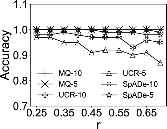 |
| (a) Length scaling |
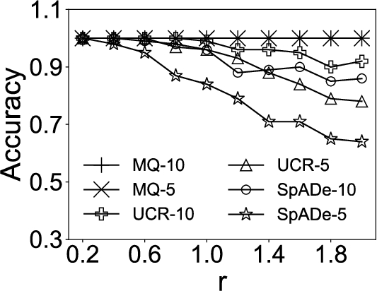 |
| (b) Amplitude scaling |
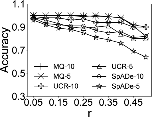 |
| (c) Shape scaling |
Let N be the number of queries in
6.3Results on Synthetic Datasets
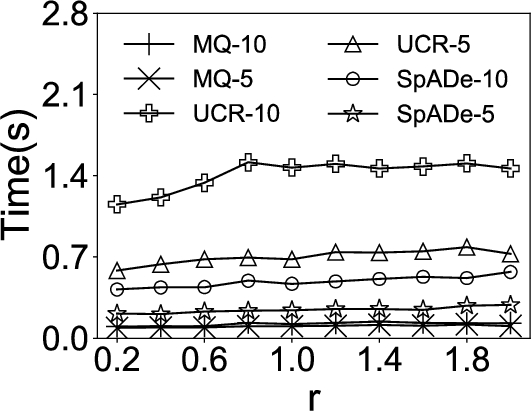
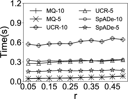
Fig. 5
Efficiency comparisons under different variations.
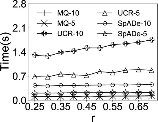 |
| (a) Length scaling |
 |
| (b) Amplitude scaling |
 |
| (c) Shape scaling |
In the first experiment, we compare our approach MQ with UCR-ED, UCR-DTW, and SpADe on synthetic datasets. Both accuracy and efficiency are tested. To compare these approaches extensively, we vary the parameter r for all three variations, length, amplitude and shape. Specifically, for the length variation, we set the maximal scaling factor r from 0.25 to 0.7 with step 0.05. For the amplitude variation, we varied r in a range of 0.2 to 2 with step 0.2. For the shape variation, we changed r in a range of 0.05 to 0.5 with step 0.05.
We set the number of queries, N, as 5 and 10, respectively. The experimental results are then indicated by MQ-5, MQ-10, UCR-DTW-5, UCR-DTW-10, SpADe-5, and SpADe-10.11 For MQ, we set the only parameter, the size of the candidate set
In each set of experiments, we attempt to find out the top-40 subsequences in the time series. The accuracy is the ratio between the number of correct subsequences and 40. Subsequence S is correct, if the overlapping ratio between S and certain planted instance exceeds the tolerance parameter,
The results are shown in Fig. 4 and Fig. 5, respectively. It can be seen that MQ outperforms UCR-DTW and SpADe in both accuracy and efficiency under all variations. The reason is that MQ summarizes common characteristics in multiple queries while the other approaches are only able to find out the subsequences that are similar to certain given query. As a consequence, when the number of query sequences N increases, UCR-DTW and SpADe yield better results. Nevertheless, UCR-DTW-10 (or SpADe-10) is twice as slow as UCR-DTW-5 (or SpADe-5) on average, which means with more query sequences provided, UCR-DTW and SpADe can find out more satisfying subsequences, but at the cost of efficiency. Instead, MQ captures latent semantics and thus demonstrates its superiority in both accuracy and efficiency under different variations. The only exception is in Fig. 4(c), where the accuracy of MQ sharply decreases when
6.4Results on Real Datasets
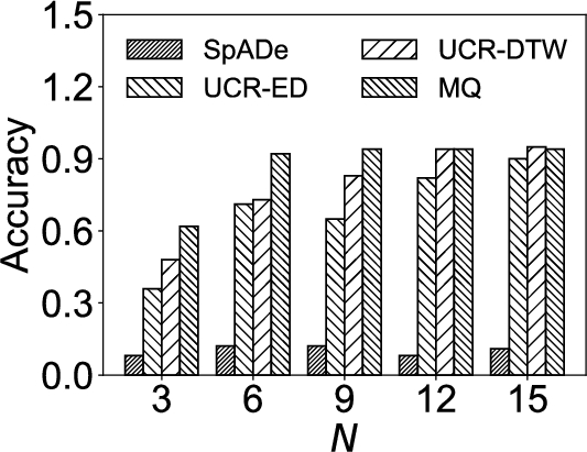
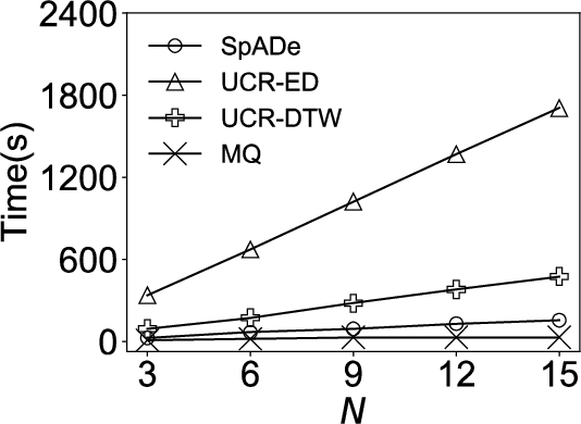
Fig. 6
Comparison on real dataset.
 |
| (a) Accuracy vs. N |
 |
| (b) Efficiency vs. N |
Fig. 7
Influence of parameter
 |
| (a) Accuracy vs. |
 |
| (b) Efficiency vs. |
In this experiment, we compare our approach with other ones as the number of query sequences N varied on real dataset. We pick out queries from the query set of size 15 so that their lengths distribute uniformly. Note that no matter the value of N, we find out top-100 subsequences from the real time series. The results are shown in Fig. 6.
It can be seen that in Fig. 6(a), the accuracy of MQ, UCR-ED, and UCR-DTW increases when N increases while the accuracy of SpADe is consistently low. The reason is that SpADe extracts local patterns by using a fixed size of sliding window, and consequently, it fails to capture the query intuition. Moreover, it is noteworthy that when
Figure 6(b) compares MQ and other approaches on efficiency. Obviously, MQ outperforms all other approaches, and its running time is insensitive to N since MQ summarizes all the queries and searches for results in the time series only once. Due to the specific pattern shape and the lack of abundant pruning strategies, UCR-ED is inferior to UCR-DTW in terms of efficiency in this dataset.
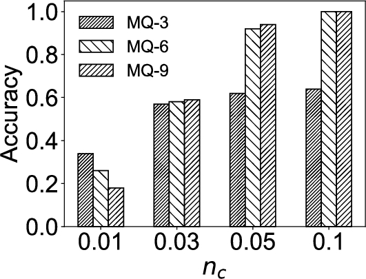
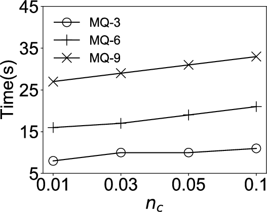
6.5Influence of Parameter n c
In this experiment, we investigate the influence of the parameter
Results are shown in Fig. 7. It can be seen that as
7Conclusions
In this paper, we have proposed a novel subsequence matching approach, Multi-querying, to reflect the query intuition. Given multiple queries, we use a multi-dimensional probability distribution to represent them. Then, a breadth-first search algorithm is then applied to finding out the top-K most similar subsequences. Extensive experiments have demonstrated that Multi-querying outperforms the state-of-the-art algorithms in terms of accuracy and performance. To the best of our knowledge, this is the first study to introduce the concept of multiple queries to express the query intuition.
Notes
1 UCR-ED is omitted for its consistent inferiority to UCR-DTW.
References
1 | Abanda, A., Mori, U., Lozano, J.A. ((2019) ). A review on distance based time series classification. Data Mining and Knowledge Discovery, 33: (2), 378–412. https://doi.org/10.1145/3514221.3526183. |
2 | Boniol, P., Palpanas, T. ((2020) ). Series2graph: Graph-based subsequence anomaly detection for time series. Proceedings of the VLDB Endowment, 13: (12), 1821–1834. https://doi.org/10.14778/3407790.3407792. |
3 | Boniol, P., Linardi, M., Roncallo, F., Palpanas, T. ((2020) ). Automated anomaly detection in large sequences. In: 2020 IEEE 36th International Conference on Data Engineering (ICDE), Dallas, TX, USA, pp. 1834–1837. https://doi.org/10.1109/ICDE48307.2020.00182. |
4 | Boniol, P., Meftah, M., Remy, E., Palpanas, T. ((2022) ). DCAM: dimension-wise class activation map for explaining multivariate data series classification. In: Proceedings of the 2022 International Conference on Management of Data, SIGMOD ’22. Association for Computing Machinery, New York, NY, USA, pp. 1175–1189. https://doi.org/10.1145/3514221.3526183. |
5 | Chen, Y., Nascimento, M.A., Ooi, B.C., Tung, A.K.H. ((2007) ). SpADe: on shape-based pattern detection in streaming time series. In: Proceedings of the 23rd International Conference on Data Engineering, ICDE 2007, The Marmara Hotel, Istanbul, Turkey, April 15–20, 2007, pp. 786–795. https://doi.org/10.1109/ICDE.2007.367924. |
6 | Dau, H.A., Bagnall, A., Kamgar, K., Yeh, C.-C.M., Zhu, Y., Gharghabi, S., Ratanamahatana, C.A., Keogh, E. ((2019) ). The UCR time series archive. IEEE/CAA Journal of Automatica Sinica, 6: (6), 1293–1305. https://doi.org/10.1109/JAS.2019.1911747. |
7 | Eravci, B., Ferhatosmanoglu, H. ((2013) ). Diversity based relevance feedback for time series search. Proceedings of the VLDB Endowment, 7: (2), 109–120. https://doi.org/10.14778/2732228.2732230. |
8 | Hu, W., Letson, F., Barthelmie, R.J., Pryor, S.C. ((2018) ). Wind gust characterization at wind turbine relevant heights in moderately complex terrain. Journal of Applied Meteorology and Climatology, 57: (7), 1459–1476. https://doi.org/10.1175/JAMC-D-18-0040.1. |
9 | Iwana, B.K., Uchida, S. ((2020) ). Time series classification using local distance-based features in multi-modal fusion networks. Pattern Recognition, 97: , 107024. https://doi.org/10.1016/j.patcog.2019.107024. https://www.sciencedirect.com/science/article/pii/S0031320319303279. |
10 | Keogh, E., Chakrabarti, K., Pazzani, M., Mehrotra, S. ((2001) ). Dimensionality reduction for fast similarity search in large time series databases. Knowledge and Information Systems, 3: (3), 263–286. https://doi.org/10.1007/PL00011669. |
11 | Kondylakis, H., Dayan, N., Zoumpatianos, K., Palpanas, T. ((2018) ). Coconut: a scalable bottom-up approach for building data series indexes. Proceedings of the VLDB Endowment, 11: (6), 677–690. https://doi.org/10.14778/3184470.3184472. |
12 | Li, Y., Tang, B., U, L.H., Yiu, M.L., Gong, Z. ((2017) ). Fast subsequence search on time series data. In: Proceedings of the 20th International Conference on Extending Database Technology, EDBT 2017, Venice, Italy, March 21–24, 2017, pp. 514–517. https://doi.org/10.5441/002/edbt.2017.58. https://openproceedings.org/2017/conf/edbt/paper-369.pdf. |
13 | Linardi, M., Palpanas, T. ((2018) ). Scalable, variable-length similarity search in data series: the ULISSE approach. Proceedings of the VLDB Endowment, 11: (13), 2236–2248. https://doi.org/10.14778/3275366.3284968. |
14 | Muthumanickam, P.K., Vrotsou, K., Cooper, M., Johansson, J. ((2016) ). Shape grammar extraction for efficient query-by-sketch pattern matching in long time series. In: 11th IEEE Conference on Visual Analytics Science and Technology, IEEE VAST 2016, Baltimore, MD, USA, October 23–28, 2016. IEEE Computer Society, pp. 121–130. https://doi.org/10.1109/VAST.2016.7883518. |
15 | Papapetrou, P., Athitsos, V., Potamias, M., Kollios, G., Gunopulos, D. ((2011) ). Embedding-based subsequence matching in time-series databases. ACM Transactions on Database Systems, 36: (3), 17–11739. |
16 | Rakthanmanon, T., Campana, B.J.L., Mueen, A., Batista, G.E.A.P.A., Westover, M.B., Zhu, Q., Zakaria, J., Keogh, E.J. ((2012) ). Searching and mining trillions of time series subsequences under dynamic time warping. In: The 18th ACM SIGKDD International Conference on Knowledge Discovery and Data Mining, KDD’12, Beijing, China, August 12–16, 2012. ACM, pp. 262–270. https://doi.org/10.1145/2339530.2339576. |
17 | Shieh, J., Keogh, E. ((2008) ). ISAX: indexing and mining terabyte sized time series. In: Proceedings of the 14th ACM SIGKDD International Conference on Knowledge Discovery and Data Mining, KDD ’08. Association for Computing Machinery, New York, NY, USA, pp. 623–631. https://doi.org/10.1145/1401890.1401966. |
18 | Wang, H., Li, C., Sun, H., Guo, Z., Bai, Y. ((2018) ). Shapelet classification algorithm based on efficient subsequence matching. Data Science Journal, 17: (6), 1–12. https://doi.org/10.5334/dsj-2018-006. |
19 | Wang, Q., Whitmarsh, S., Navarro, V., Palpanas, T. ((2022) ). IEDeaL: a deep learning framework for detecting highly imbalanced interictal epileptiform discharges. Proceedings of the VLDB Endowment, 16: (3), 480–490. https://doi.org/10.14778/3570690.3570698. |
20 | Wasay, A., Wei, X., Dayan, N., Idreos, S. ((2017) ). Data canopy: accelerating exploratory statistical analysis. In: Proceedings of the 2017 ACM International Conference on Management of Data, SIGMOD Conference 2017, Chicago, IL, USA, May 14–19, 2017, ACM, pp. 557–572. https://doi.org/10.1145/3035918.3064051. |
21 | Wu, J., Wang, P., Pan, N., Wang, C., Wang, W., Wang, J. ((2019) ). KV-match: a subsequence matching approach supporting normalization and time warping. In: 35th IEEE International Conference on Data Engineering, ICDE 2019, Macao, China, April 8–11, 2019. IEEE, pp. 866–877. https://doi.org/10.1109/ICDE.2019.00082. |
22 | Zoumpatianos, K., Idreos, S., Palpanas, T. ((2016) ). ADS: the adaptive data series index. VLDB Endowment, 25: (6), 843–866. https://doi.org/10.1007/s00778-016-0442-5. |


