Burst Ratio of Packet Losses in Individual Network Flows

1Introduction

The burst ratio characteristic, B, was proposed in McGowan (2005). It is computed by dividing the mean length of the sequence of losses observed in a stream of interest, by the hypothetical mean length of the sequence of losses in the Bernoulli process, i.e. in a process with all losses being purely random, uncorrelated, and of the same probability L.

We denote the mean length of the sequence of losses observed in a stream of interest by G‾, while the hypothetical mean length in the Bernoulli process by K‾. Therefore, by definition:

For illustration, let us consider an example of the following stream of 16 packets: 1 1 0 1 1 1 1 1 0 0 0 1 1 1 1 1. Herein, 1 corresponds to a successful packet transmission, 0 to a packet loss. We check quickly that the overall loss probability (loss ratio) is L=4/16=1/4. Thus, the hypothetical mean length of the sequence of zeroes in the Bernoulli process with L=1/4 should be K‾=(1−L)−1=4/3. However, in our stream there are two sequences of zeroes, of lengths 1 and 3, respectively. Hence the mean length of the sequence of zeroes is G‾=2, which gives B=G‾/K‾=1.5. This means that a sequence of losses in the stream is on average 1.5 times longer, than in the case when the losses are independent of each other.

Experiments indicate that G‾ is typically 1.5–2.0 times greater than K‾ in contemporary packet networks (Chydzinski and Samociuk, 2019; Samociuk et al., 2019). Therefore, there must exist a mechanism causing the dependency between losses of consecutive packets, i.e. making the probability of losing a packet higher, if the previous packet has been lost. In fact, this mechanism is the same mechanism which causes losses in general, i.e. buffer overflow events in routers and switches. Namely, when the output buffer of a networking device is overflowed, each incoming packet is deleted. This overflow state may last for some time, until a room in the buffer is freed. Therefore, during such an overflow state, several packets can be lost in a row, creating a sequence of losses.

The elevated values of the burst ratio in contemporary networks and the Internet influence negatively the quality of experience provided by multimedia streams, in particular those of real-time character. Losing occasionally a long sequence of video or audio packets can degrade the quality of experience more than losing short sequences even if the latter happens more frequently. This is due to human perception characteristics and codecs used in real-time multimedia transmissions. For some types of transmissions, this phenomenon has a precise mathematical model. Namely, on page 8 of ITU-T (2015) we can find a formula which expresses the degradation of the quality of voice transmission in the Internet telephony, as a function of the burst ratio.

In this article, we investigate the burst ratio in the per-flow manner, i.e. individually for every flow of packets traversing a network node. We first confront all the per-flow burst ratios with each other, as well as with the burst ratio computed for the multiplexed traffic. Next, we study the influence of different features of the system on these burst ratios. In particular, the influence of rates of flows and their mutual proportions, as well as the standard deviation of interarrival times, the capacity of the buffer, the system load and the distribution of the service time, is studied. We pay special attention to non-Poisson models of flows, for the reasons discussed below.

As it will be shown in the next section, so far the burst ratio literature has been devoted mainly to analysis of the multiplexed traffic. However, it is easy to understand that burst ratios in individual flows are even more important. Indeed, the quality of multimedia perceived by an end user depends on the burst ratio in the multimedia flow of this user only, not on the burst ratio in the multiplexed traffic.

Note that it is very difficult to predict if the burst ratio of a particular flow should be smaller than, greater than or equal to the burst ratio of the multiplexed traffic. This is because two different phenomenons, playing against each other, can be thought about. First, a sequence of losses in the multiplexed traffic can be composed of losses from a few flows, so the subsequence of losses in each particular flow can be shorter. That said, a sequence of packet losses in a flow may happen even if there is no such sequence in the multiplexed traffic. Consider, for example, the following sequence of 8 packets belonging to 2 flows: 0 1 0 1 0 1 0 1. Let every odd packet in this sequence belong to the first flow, while every even packet belongs to the second flow. Obviously, in the first flow there is a sequence of 4 packets lost consecutively, but in the multiplexed traffic no sequence of losses can be noticed.

The mathematical analysis of the per-flow burst ratio in the general model, with non-Poisson flows and general service time distribution, is extremely hard. It is not an overstatement to say that we cannot expect to have an analytical solution of such model in a foreseeable future. This follows from the fact that a much simpler model, i.e. the G/G/1 queue with a finite buffer, has no exact analytical solution so far, even though it has been studied by many researchers for many years. The G/G/1 model has only one arrival stream of general type. In the model considered herein, there are N such streams, each perhaps with a different interarrival time distribution. This makes it far more difficult than the unsolved G/G/1 model. On the other hand, it is well known that the network traffic is usually non-Poisson, and the error made when using the simplified Poisson model in the performance evaluation can be huge (Leland et al., 1994; Paxson and Floyd, 1995). Therefore, it is important to use a model with the general interarrival time distribution for every flow.

For these reasons, the individual burst ratios are studied herein by means of the Omnet++ simulation framework, OpenSim Ltd. (2019). This is a modern, discrete-event simulation framework of modular architecture, which allows for programming, directly in C++, simulators of very high performance. In our simulator, tens of millions of packets were simulated in each simulation run, which was enough to eliminate random fluctuations of the results. At the same time, we were not restricted to any type of the interarrival time distribution within each flow.

The remainder of the paper is divided into five sections. Namely, in Section 2, the related work is characterized. In Section 3, the model of the queueing system, as well as the mathematical notations, are introduced. The known results for the Poisson traffic are recalled in Section 4. Then, the new results on the per-flow burst ratios, including several non-Poisson scenarios, are shown and discussed in Section 5. The final conclusions are drawn in Section 6.

This article is an extended version of paper by Chydzinski and Adamczyk (2022), presented during 10th World Conference on Information Systems and Technologies, 12–14 April, Budva, 2022.

2Related Work

Notice first that to compute B by means of (2), we need to know L. The loss ratio is not only required to calculate the burst ratio, but is also a fundamental parameter of the loss process on its own. Therefore, it was studied extensively in many papers, using direct packet loss measurements, (e.g. Bolot, 1993; Coates and Nowak, 2000; Duffield et al., 2001; Benko and Veres, 2002; Sommers et al., 2005; Lan et al., 2019), or theoretical models (e.g. Yajnik et al., 1999; Sanneck and Carle, 1999; Yu et al., 2005; Hasslinger and Hohlfeld, 2008; Chydzinski and Adamczyk, 2012; Jelassi and Rubino, 2018).

The burst ratio was introduced in McGowan (2005). It was then analysed in Rachwalski and Papir (2014, 2015) by means of a simple Markov model with two states. In these studies, an abstract random process (the Markov chain) was exploited to imitate the stochastic structure of the loss process, while the real reason of losses, an overflowed buffer, was not present in the model.

Then, the burst ratio was studied in Chydzinski and Samociuk (2019), Chydzinski et al. (2018b), Chydzinski (2022) using as model an overflowed buffer. In these studies, B was derived for a few kinds of Poisson streams. In particular, the multiplexed burst ratio for single Poisson arrivals was found in Chydzinski and Samociuk (2019), while for batch Poisson arrivals in Chydzinski et al. (2018b). The per-flow burst ratio for Poisson arrivals was derived in Chydzinski (2022). Moreover, in Samociuk et al. (2019) the multiplexed burst ratio was studied experimentally in a real networking environment, i.e. in an academic network of a large university, which operated normally during the measurements.

It is perhaps worth mentioning that the structure of losses can be characterized by means of other characteristics as well. For instance, in Cidon et al. (1993) the probability of having m losses in a block of n consecutive packets was calculated. In Bratiychuk and Chydzinski (2009), the distribution of the length of the first sequence of losses was analysed. However, the burst ratio seems to have the simplest and most intuitive interpretation when characterizing the inclination of losses to occur one after another.

Finally, in a few papers the possibility of decreasing the burst ratio value in TCP/IP networks has been studied. One of the approaches to achieve this goal is to exploit active queue management in the buffers of networking devices. Application of AQM is advocated anyway, for other important reasons, by Internet Engineering Task Force, Baker and Fairhurst (2015). There is a variety of proposed AQM methods and algorithms (see e.g. Nichols and Jacobson, 2012; Khoshnevisan and Salmasi, 2016; Wang et al., 2017; Kahe and Jahangir, 2019; Feng et al., 2017; Hotchi et al., 2020), but having mitigation of the burst ratio in mind, the algorithms based on the dropping function (Chydzinski et al., 2018a; Patel and Karmeshu, 2019), can be particularly beneficial.

3The Model

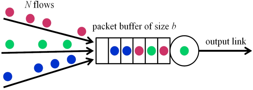
We deal herein with the following model of the queue. The packets from N separate flows arrive to the output interface of a router, where they are placed in a buffer of capacity b, see Fig. 1. All these packets are kept in the buffer before further transmission, which is conducted in the arrival order (FIFO), regardless to which flow a packet belongs to. If an arriving packet finds the buffer full, it is lost (deleted). We adopt the convention that the service position is included in b.

The service time of a packet has some distribution, which is not specified and can assume any form. Its distribution function is denoted by F, the mean service time by E(F), the standard deviation of the service time by D(F).

An i-th flow has its own interarrival time distribution, with the distribution function denoted by Gi, which can assume any form. The mean interarrival time of the i-th flow will be denoted by E(Gi). The rate of the i-th flow will be denoted by:

Fig. 1

The model of the queuing system.

The burst ratio of packet losses of an i-th flow will be denoted by Bi. The burst ratio for the whole multiplexed traffic will be denoted by B. Analogously, Li will stand for the individual loss ratio of an i-th flow, while L for loss ratio of the multiplexed traffic.

We will use the following notation throughout the paper. The total arrival rate, λ, is:

4Analytical Background

If all flows are Poisson, then it is possible to derive the burst ratio for the multiplexed traffic, as well as for individual flows. In this section, we assume that there are N Poisson flows of rates λ1,…,λN, respectively. Thus the multiplexed traffic is also Poisson.

5Experiments’ Results and Discussions

Unfortunately, as it was discussed in Section 1, the traffic in networks is often far from Poisson, and there is little hope to find analytical solutions for the non-Poisson model. Therefore, the results presented in this section were obtained by means of Omnet++ simulation framework. We are especially interested in the results obtained for non-Poisson flow models. Sometimes, however, results for Poisson flows are shown as well, to demonstrate the differences between the two types.

In every simulation run, 50 million packets were simulated. If not stated otherwise, the buffer capacity was 50, the queue was fully loaded (ρ=1), and the service time was exponential. Exceptions are clearly indicated and concern the cases when the impact of the buffer capacity, the variance of the service time and the load were studied.

5.2Flows of the Same Rates but Distinct Distributions

In this set of simulations, flows of the same rate, but distinct distributions of the interarrival time were investigated.

Firstly, we multiplexed two flows with very different variances of the interarrival time (0 and 20). Namely, in the first flow a constant interarrival time of 2 was used, whilst in the second flow, it was distributed Γ(0.2,10). The resulting burst ratios were quite surprising: B=2.69, B1=1.32 and B2=2.73. Specifically, the first individual burst ratio is less than the multiplexed one, but the second individual burst ratio is greater than the two of them, i.e. B1<B<B2. This can be interpreted as a result of the interplay of the two phenomenons discussed in Section 1 – the one making Bj smaller than B, while the other making Bj larger than B. Apparently, in this experiment the latter phenomenon prevailed in the case of the second flow. It is also worth mentioning, that the loss ratios behaved in a similar way. We obtained L=0.033, L1=0.015 and L2=0.050. Therefore, L2 is significantly larger than L1 and it holds L1<L<L2. This is not possible in the all-Poisson model, in which it is L1=⋯=Lj=L in every case (see (24)).

Next, we checked a scenario with three flows, each having a different, but moderate variance of the interarrival time. Namely, the interarrival times distributions were exponential with the parameter 1/3, uniform on (2,4) and Γ(3,1), respectively. The following results were obtained: B=1.77, B1=1.53, B2=1.28, B3=1.36. As we can see, not necessarily one or more of the per-flow burst ratios must be larger than B, even when the distributions of interarrival times are substantially different. In scenarios with distributions of interarrival times having small or moderate variances, we can expect per-flow burst ratios to be less than the multiplexed burst ratio.

What is even more interesting, even in the case when some flows have large variances of the interarrival time, all the per-flow burst ratios can be quite small and less than the multiplexed one. It happens, however, when the number of flows is not small and no flow with a large variance dominates the mix. This effect was observed in the scenario with N=10 and the interarrival service times distributed as: Γ(100/1,1/10), Γ(100/4,4/10), Γ(100/9,9/10),…, Γ(100/100,100/10). The distributions were chosen in such a way that λ1=⋯=λ10=1/10, but the standard deviations of the interarrival times were 1,2,3,…,10 in flows 1,2,3,…,10, respectively. The resulting multiplexed burst ratio was 1.81, while the per-flow burst ratios are depicted in Fig. 2. As it can be observed, all per-flow burst ratios are significantly smaller than B, and not very different from each other, even though the variances of the flows differ by far. The per-flow loss ratios behave in a similar way, as is depicted in Fig. 3 – there are relatively small differences between them.

Fig. 2

Burst ratios for 10 flows of the same rates but standard deviations growing from 1 to 10.

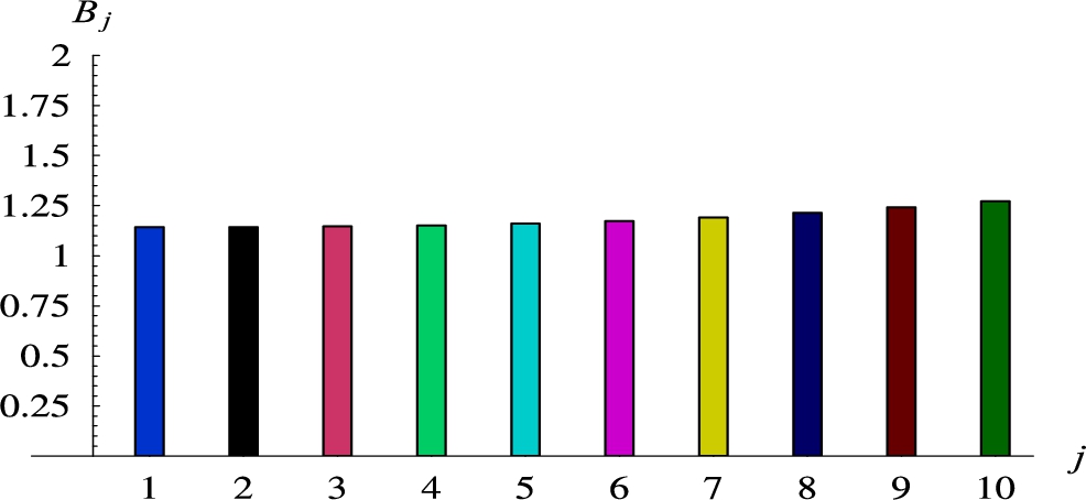
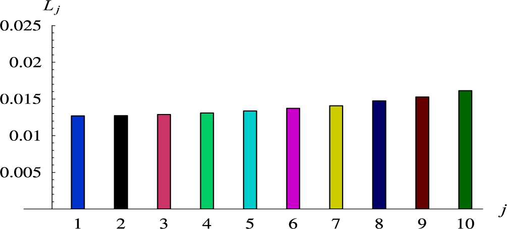
Fig. 3

Loss ratios for 10 flows of the same rates but standard deviations growing from 1 to 10.

At this point, the following essential questions emerge: can all per-flow burst ratios be larger than the multiplexed burst ratio? Or all equal to B? These problems are so far unresolved. We were not able to devise scenarios producing such outputs. On the other hand, the possibility of having such results is difficult to exclude analytically.

5.3Flows of Different Rates

In the next group of experiments, we tested flows of different rates, but with distributions of the interarrival times of the same type.

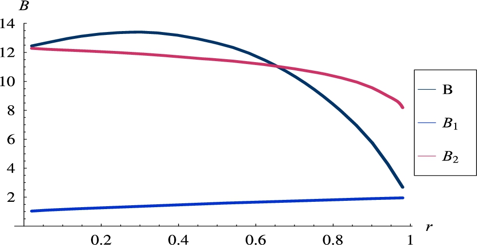
Firstly, two Poisson flows were exploited, with variable proportions between their rates. In particular, the rate of the first flow was equal to r, whilst the rate of the second flow was 1−r. The value of r was then increased from 0.01 to 0.99. The results, i.e. B1, B2 and B versus r, are presented in Fig. 4. (They were also confirmed via Theorems 1 and 2.) As we can observe in Fig. 4, the multiplexed B is constant, but the individual burst ratio depends severely on the flow rate, in a monotonic way. The larger the rate, the larger Bi. For small rates, Bi approaches 1, while for rates near 1, Bi approaches B.

Fig. 4

Burst ratios versus the rate of the first flow. Poisson flows, λ1=r, λ2=1−r.

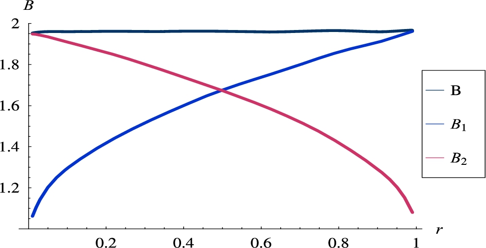
In the second scenario, we used two non-Poisson flows of different proportions. Namely, the interarrival time was distributed Γ(1,1/r) in the first flow and Γ(0.01,100/(1−r)) in the second flow. Thus we had again λ1=r, λ2=1−r, but this time for non-Poisson flows. The resulting burst ratios are depicted in Fig. 5.

As it can be observed, the figure is quite different than in the all-Poisson case. First of all, we have B2>B1 for every r. This can be assigned to the larger variance in the second flow. Secondly, B1 and B2 do not vary as much in Fig. 5, as in Fig. 4. On the other hand, B varies much more in Fig. 5, than in Fig. 4. Moreover, the B2 and B curves intersect around r=0.66. This demonstrates the possibility of having exactly the same multiplexed burst ratio and the per-flow burst ratio in one of the flows. The examples with Bj<B and Bj>B were already given in the previous subsection, but they are also visible in Fig. 5, for r<0.66 and r>0.66, respectively.

Fig. 5

Burst ratios versus the rate of the first flow. Non-Poisson flows, λ1=r, λ2=1−r.

In the last scenario in this group, we tested three non-Poisson flows of rates different by an order and two orders of magnitude. Namely, flows with the distributions of the interarrival times Γ(0.11235955,10), Γ(1,10), and Γ(10,10) were used, which resulted in the rates of 0.89, 0.1 and 0.01, respectively. The results were as follows: B=3.92, B1=3.94, B2=1.22 and B3=1.01. Therefore, all the flows had different burst ratios, with the very high burst ratio of the first flow. However, it must be stressed that the very high B1 is not caused by the high variance of the first flow only. It is caused by its high variance and high λ1. This is easy to see if we observe that the second flow has an even higher variance than the first flow, but B2 is rather small, due to small λ2.

5.4Influence of the Buffer Capacity

In the next scenarios, we checked how the buffer capacity influences the individual and multiplexed burst ratios. In particular, three flows having the distributions of interarrival times Γ(0.3,10), exponential with the average of 3 and uniform on (2,4), respectively, were assumed. Hence the flows had a common rate, but significantly different variances. The buffer capacity was increased from 1 to 100. The results, i.e. B1, B2 and B versus the buffer capacity, are presented in Fig. 6.

Fig. 6

Burst ratios versus the buffer capacity.

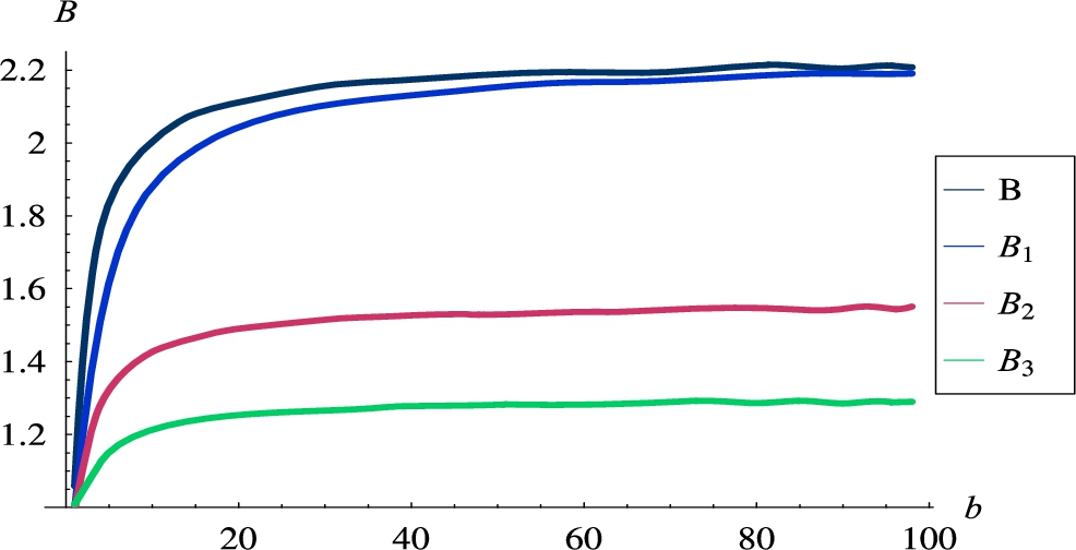
We can notice in Fig. 6 that the capacity of the buffer had the same influence on every burst ratio. When the buffer was very small, every burst ratio got close to 1. Apparently, a small capacity of the buffer makes the loss process less correlated, regardless if we consider the losses in an individual flow or in the multiplexed traffic. We can also notice in Fig. 6 that all the burst ratios grew with the capacity of the buffer, but not forever. At the capacity around 40, the curves became flat and the burst ratios did not change anymore, regardless of how big the buffer was.

5.5Influence of the Service Time

In the next experiment, we tested the influence of the distribution of the service time on the burst ratios.

The same three flows, as in the previous subsection, were assumed (gamma, exponential, uniform). The distribution of the service time was Γ(p,1p), where p>0 was a parameter. In this way the mean service time was equal to 1, regardless of the value of p. On the other hand, the standard deviation was D(F)=1p. Therefore, manipulating p, we could obtain an arbitrary value of this standard deviation. The results obtained for D(F)∈(0,10) are shown in Fig. 7.

Fig. 7

Burst ratios as functions of the standard deviation of the service time.

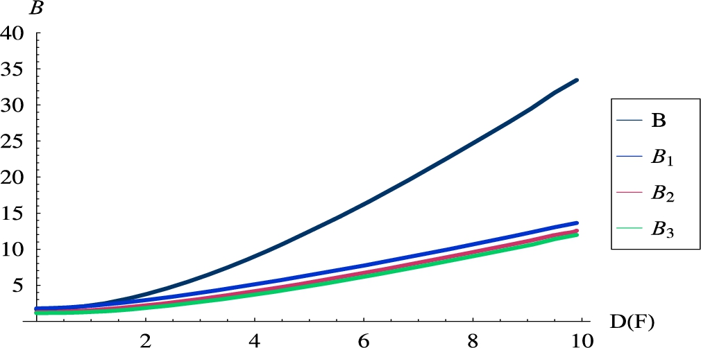
As it can be seen in the figure, the standard deviation of the service time had a strong influence on the burst ratios. Note that extreme values of Bi and B were reached – about 30 for the multiplexed traffic and about 10 for single flows. What is worth emphasizing, all the per-flow curves are rather close to each other. This means that the influence of the service time distribution was so strong, that it attenuated to the differences in per-flow results caused by quite different interarrival time distributions among flows.

5.6Impact of the Load

In the last set of experiments, we studied the dependence of the burst ratios on the load of the queue. The same 3 flows, as in Section 5.4, were used, i.e. all with the rate of 1/3, but different variances. The service time was Γ(1/25,25) distributed, scaled additionally by the factor ρ, where ρ varied from 0.5 to 2.5, i.e. from a strong underload to a strong overload. Two buffer sizes, 20 and 50, were used.

The resulting burst ratios for b=20 are depicted in Fig. 8, while for b=50, in Fig. 9. As can be seen in these figures, the load has a much weaker influence on the burst ratios than the variance of the service time or the buffer capacity, discussed above. This influence gets stronger when the buffer capacity grows – we can see more variability in Fig. 9 than in Fig. 8. This is only true, however, for small or moderate buffers. For large buffers, the burst ratios stabilize and do not change anymore when the buffer grows, as it was demonstrated in Fig. 7.

Fig. 8

Burst ratios versus the system load, b=20.

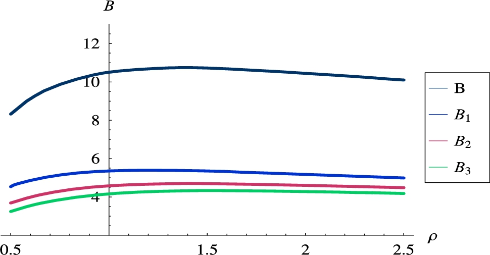
Fig. 9

Burst ratios versus the system load, b=50.

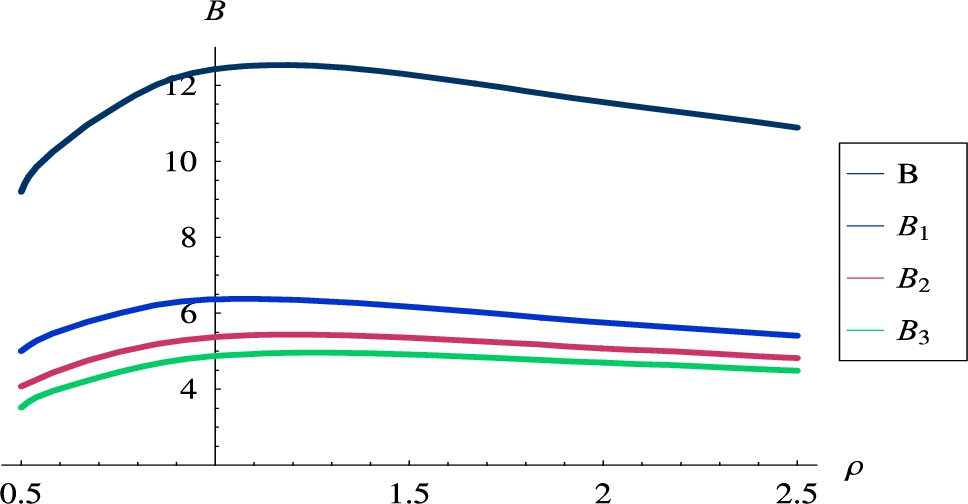
Finally, we can observe local maxima in Figs. 8 and 9, both for multiplexed and individual burst ratios. These maxima occur for some ρ>1 in the case of b=20, while for b=50 they get close to ρ=1, but are not exactly at 1.

6Conclusions

In this paper, we studied the burst ratio of packet losses at a TCP/IP network node. The main contribution of the paper consists of:

In particular, the following observations were made in the simulations.

The burst ratio of a particular flows was smaller than, greater than, or equal to the multiplexed burst ratio, depending on types of involved flows. Most often we had, however, Bj<B for every j. Bj>B happened when the flow of interest had a large variance of the interarrival time and occupied a large portion of the total load at the same time. Many flows of very different or even large variances did not lead to Bj>B, if all the rates were small. It is unknown whether a scenario with Bj>B for every j is possible, or a scenario with B1=⋯=BN=B. We could not devise such scenarios. On the other hand, the possibility of having such results is difficult to exclude analytically. This is one of the possible subjects of future work.

In the scenarios with all flows being stochastically the same, every Bj was smaller than B. Moreover, every Bj decreased with N. In the scenarios with flows having different interarrival time distributions, the per-flow burst ratios could differ by far, even if all the flows had the same rate.

The individual burst ratio was easily affected by the variance of the distribution of the interarrival time. The greater was this variance in one or more flows, the larger the individual burst ratios were. Moreover, the individual burst ratios were susceptible to changes of the buffer capacity. When this capacity was small, every Bj approached 1. Then every Bj grew fast with the capacity of the buffer, but not forever. At some moderate buffer capacity, the burst ratios stopped growing and stabilized. The service time variance had a deep influence on the individual burst ratios, deeper than all the remaining studied factors. Finally, the load of the queue had a mild impact on the per-flow burst ratios, even when considered in the range from a severe underload of ρ=0.5, to a severe overload of ρ=2.5. This impact was even weaker in a scenario with a small buffer.

When comparing scenarios with Poisson and non-Poisson flows, several significant differences were noted. Firstly, Bj>B was never observed in a pure Poisson model. As it was demonstrated, such a case is possible in a non-Poisson model. Secondly, in a pure Poisson model, all the per-flow burst ratios are the same when the rates are the same. The per-flow burst ratios can differ by far for flows of the same rates, but different, non-Poisson types. Thirdly, in a pure Poisson model, all the loss ratios are equal to each other, even if the rates are different. Such a case is rare in non-Poisson models, in which all the loss ratios are usually different from each other, even if the arrival rates are the same. These observations indicate that the pure Poisson model, for which the analytical solutions are available, should be applied very carefully and only when the statistical characteristics of flows are not far from Poisson.

An interesting future work would be the per-flow analysis of the queueing delay (waiting time), instead of losses. We have seen here that loss characteristics (burst ratio and loss ratio) may differ significantly among flows, depending on system parameters. The same can be suspected about the distribution of the waiting time perceived by packets belonging to different flows.

Another recommendation for future work could be the per-flow analysis of losses (and perhaps delays) in an extended model, incorporating active queue management at the buffer. Herein, we dealt only with the classic, tail-drop buffer management. It is intuitively clear that AQM must have a deep impact on the per-flow characteristics, but further research is needed to study this effect in detail, depending on the type of AQM used.

References

1 | Baker, F., Fairhurst, G. (2015). IETF Recommendations Regarding Active Queue Management. Request for Comments RFC 7567, Internet Engineering Task Force. https://doi.org/10.17487/RFC7567. |
2 | Benko, P., Veres, A. ((2002) ). A passive method for estimating end-to-end TCP packet loss. In: IEEE Global Telecommunications Conference, 2002. GLOBECOM ’02, Vol. 3: , pp. 2609–26133. https://doi.org/10.1109/GLOCOM.2002.1189102. |
3 | Bolot, J.-C. ((1993) ). End-to-end packet delay and loss behavior in the internet. In: Conference Proceedings on Communications Architectures, Protocols and Applications, SIGCOMM ’93. Association for Computing Machinery, New York, NY, USA, pp. 289–298. 978-0-89791-619-6. https://doi.org/10.1145/166237.166265. |
4 | Bratiychuk, M., Chydzinski, A. ((2009) ). On the loss process in a batch arrival queue. Applied Mathematical Modelling, 33: (9), 3565–3577. https://doi.org/10.1016/j.apm.2008.11.015. |
5 | Chydzinski, A. ((2022) ). Per-flow structure of losses in a finite-buffer queue. Applied Mathematics and Computation, 428: , 127215. https://doi.org/10.1016/j.amc.2022.127215. |
6 | Chydzinski, A., Adamczyk, B. ((2012) ). Transient and stationary losses in a finite-buffer queue with batch arrivals. Mathematical Problems in Engineering, 2012: , 1–17. https://doi.org/10.1155/2012/326830. |
7 | Chydzinski, A., Adamczyk, B. ((2022) ). Burst ratios of individual flows. In: Rocha, A., Adeli, H., Dzemyda, G., Moreira, F. (Eds.), Information Systems and Technologies, Lecture Notes in Networks and Systems. Springer International Publishing, Cham, pp. 372–381. 978-3-031-04829-6. https://doi.org/10.1007/978-3-031-04829-6_33. |
8 | Chydzinski, A., Samociuk, D. ((2019) ). Burst ratio in a single-server queue. Telecommunication Systems, 70: (2), 263–276. https://doi.org/10.1007/s11235-018-0476-7. |
9 | Chydzinski, A., Barczyk, M., Samociuk, D. ((2018) a). The single-server queue with the dropping function and infinite buffer. Mathematical Problems in Engineering, 2018: , 3260428. https://doi.org/10.1155/2018/3260428. |
10 | Chydzinski, A., Samociuk, D., Adamczyk, B. ((2018) b). Burst ratio in the finite-buffer queue with batch poisson arrivals. Applied Mathematics and Computation, 330: , 225–238. https://doi.org/10.1016/j.amc.2018.02.021. |
11 | Cidon, I., Khamisy, A., Sidi, M. ((1993) ). Analysis of packet loss processes in high-speed networks. IEEE Transactions on Information Theory, 39: (1), 98–108. https://doi.org/10.1109/18.179347. |
12 | Coates, M.J., Nowak, R.D. ((2000) ). Network loss inference using unicast end-to-end measurement. In: ITC Conference on IP Traffic, Modeling and Management, Monterey, CA, pp. 281–289. |
13 | Duffield, N.G., Lo Presti, F., Paxson, V., Towsley, D. ((2001) ). Inferring link loss using striped unicast probes. In: Proceedings IEEE INFOCOM 2001, Conference on Computer Communications, Twentieth Annual Joint Conference of the IEEE Computer and Communications Society (Cat. No.01CH37213), Vol. 2: , pp. 915–9232. https://doi.org/10.1109/INFCOM.2001.916283. |
14 | Feng, C.-W., Huang, L.-F., Xu, C., Chang, Y.-C. ((2017) ). Congestion control scheme performance analysis based on nonlinear RED. IEEE Systems Journal, 11: (4), 2247–2254. https://doi.org/10.1109/JSYST.2014.2375314. |
15 | Hasslinger, G., Hohlfeld, O. ((2008) ). The Gilbert-Elliott model for packet loss in real time services on the internet. In: 14th GI/ITG Conference – Measurement, Modelling and Evalutation of Computer and Communication Systems, pp. 1–15. |
16 | Hotchi, R., Chibana, H., Iwai, T., Kubo, R. ((2020) ). Active queue management supporting TCP flows using disturbance observer and Smith predictor. IEEE Access, 8: , 173401–173413. https://doi.org/10.1109/ACCESS.2020.3025680. |
17 | ITU-T (2015). The E-model: A Computational Model for Use in Transmission Planning. Recommendation G.107, International Telecommunication Union. |
18 | Jelassi, S., Rubino, G. ((2018) ). A perception-oriented Markov model of loss incidents observed over VoIP networks. Computer Communications, 128: , 80–94. https://doi.org/10.1016/j.comcom.2018.06.009. |
19 | Kahe, G., Jahangir, A.H. ((2019) ). A self-tuning controller for queuing delay regulation in TCP/AQM networks. Telecommunication Systems, 71: (2), 215–229. https://doi.org/10.1007/s11235-018-0526-1. |
20 | Khoshnevisan, L., Salmasi, F.R. ((2016) ). A robust and high-performance queue management controller for large round trip time networks. International Journal of Systems Science, 47: (7), 1586–1597. https://doi.org/10.1080/00207721.2014.941959. |
21 | Lan, H., Ding, W., Zhang, Y. ((2019) ). Strengthening packet loss measurement from the network intermediate point. KSII Transactions on Internet and Information Systems (TIIS), 13: (12), 5948–5971. https://doi.org/10.3837/tiis.2019.12.009. |
22 | Leland, W.E., Taqqu, M.S., Willinger, W., Wilson, D.V. ((1994) ). On the self-similar nature of ethernet traffic (extended version). IEEE/ACM Transactions on Networking, 2: (1), 1–15. https://doi.org/10.1109/90.282603. |
23 | McGowan, J.W. (2005). Burst Ratio: A Measure of Bursty Loss on Packet-Based Networks. US6931017B2, August 2005. |
24 | Nichols, K., Jacobson, V. ((2012) ). Controlling Queue Delay: a modern AQM is just one piece of the solution to bufferbloat. Queue, 10: (5), 20–34. https://doi.org/10.1145/2208917.2209336. |
25 | OpenSim Ltd. (2019). OMNeT++ Discrete Event Simulator. https://omnetpp.org/. |
26 | Patel, S., Karmeshu ((2019) ). A new modified dropping function for congested AQM networks. Wireless Personal Communications, 104: (1), 37–55. https://doi.org/10.1007/s11277-018-6007-8. |
27 | Paxson, V., Floyd, S. ((1995) ). Wide area traffic: the failure of Poisson modeling. IEEE/ACM Transactions on Networking, 3: (3), 226–244. https://doi.org/10.1109/90.392383. |
28 | Rachwalski, J., Papir, Z. ((2014) ). Burst ratio in concatenated Markov-based channels. Journal of Telecommunications and Information Technology, 1: , 3–9. |
29 | Rachwalski, J., Papir, Z. ((2015) ). Analysis of burst ratio in concatenated channels. Journal of Telecommunications and Information Technology, 4: , 65–73. |
30 | Samociuk, D., Barczyk, M., Chydzinski, A. ((2019) ). Measuring and analyzing the burst ratio in IP traffic. In: Li, Q., Song, S., Li, R., Xu, Y., Xi, W., Gao, H. (Eds.), Broadband Communications, Networks, and Systems, Lecture Notes of the Institute for Computer Sciences, Social Informatics and Telecommunications Engineering. Springer International Publishing, Cham, pp. 86–101. 978-3-030-36442-7. https://doi.org/10.1007/978-3-030-36442-7_6. |
31 | Sanneck, H.A., Carle, G. ((1999) ). Framework model for packet loss metrics based on loss runlengths. In: Multimedia Computing and Networking 2000, Vol. 3969: . SPIE, San Jose, CA, USA, pp. 177–187. https://doi.org/10.1117/12.373520. |
32 | Sommers, J., Barford, P., Duffield, N., Ron, A. ((2005) ). Improving accuracy in end-to-end packet loss measurement. In: Proceedings of the 2005 Conference on Applications, Technologies, Architectures, and Protocols for Computer Communications, SIGCOMM ’05. Association for Computing Machinery, New York, NY, USA, pp. 157–168. 978-1-59593-009-5. https://doi.org/10.1145/1080091.1080111. |
33 | Wang, P., Zhu, D., Lu, X. ((2017) ). Active queue management algorithm based on data-driven predictive control. Telecommunication Systems, 64: (1), 103–111. https://doi.org/10.1007/s11235-016-0162-6. |
34 | Wolff, R.W. ((1982) ). Poisson arrivals see time averages. Operations Research, 30: (2), 223–231. |
35 | Yajnik, M., Moon, S., Kurose, J., Towsley, D. ((1999) ). Measurement and modelling of the temporal dependence in packet loss. In: IEEE INFOCOM ’99. Conference on Computer Communications, Proceedings. Eighteenth Annual Joint Conference of the IEEE Computer and Communications Societies. The Future Is Now (Cat. No.99CH36320), Vol. 1: , pp. 345–3521. https://doi.org/10.1109/INFCOM.1999.749301. |
36 | Yu, X., Modestino, J.W., Tian, X. ((2005) ). The accuracy of Gilbert models in predicting packet-loss statistics for a single-multiplexer network model. In: Proceedings IEEE 24th Annual Joint Conference of the IEEE Computer and Communications Societies, Vol. 4: , pp. 2602–2612. https://doi.org/10.1109/INFCOM.2005.1498544. |