
Novel Entropy Measure Definitions and Their Uses in a Modified Combinative Distance-Based Assessment (CODAS) Method Under Picture Fuzzy Environment
Abstract
From the perspective of multiple attribute decision analysis, the evaluation of decision alternatives should be based on the performance scores determined with respect to more than one attribute. Fuzzy logic concepts can equip the evaluation process with different scales of linguistic terms to let the decision-makers point out their ideas and preferences. A more recent one of fuzzy sets is the picture fuzzy set which covers three separately allocable elements: positive, neutral, and negative membership degrees. The novel and distinctive element included by a picture fuzzy set is the refusal degree which is equal to the difference between 1 and the sum of the other three. In this study, we aim to contribute to the literature of the picture fuzzy sets by (i) proposing two novel entropy measures that can be used in objective attribute weighting and (ii) developing a novel picture fuzzy version of CODAS (COmbinative Distance-based ASsessment) method which is empowered with entropy-based attribute weighting. The applicability of the method is shown in a green supplier selection problem. To clarify the differences of the proposed method, a comparative analysis is provided by considering traditional CODAS, spherical fuzzy CODAS, and spherical fuzzy TOPSIS with different entropy-based scenarios.
1Introduction
Many Multiple Attribute Decision Making (MADM) problems do not involve appropriate data which are directly measurable such as cost, net profit, any financial ratio, volume or weight of an item, etc. To deal with the quantification problems, the decision-makers can benefit from linguistic terms in stating their thoughts and preferences regarding the problem. Linguistic terms are often defined in different fuzzy environments. Zadeh (1965) launched the domain of fuzzy sets for symbolizing human judgments. In conventional fuzzy set definition, the opinions can be represented by a single membership degree (μ) which ranges between 0 and 1. This membership degree measures the optimism or agreement level and possesses a positive perspective.
To smooth the representation challenge of the uncertainty in human judgments, fuzzy set domain has been extended by researchers from different fields. Atanassov (1986) introduced the intuitionistic fuzzy sets (IFS) by defining a negative membership (or non-membership) degree (v). This new element in the fuzzy set definition brings resilience to the uncertainty representation issue because the experts are able to specify their pessimistic views or disagreements in this way. Hence, non-membership degree points out a negative perspective. Atanassov (1986) also defined a new element regarding the indeterminacy (or hesitancy) which shows the experts’ neutral preference:
After the introduction of the horizon widening features of fuzzy sets and IFSs, new fuzzy concepts have been proposed in the literature. Pythagorean fuzzy sets (Yager, 2013), q-Rung orthopair fuzzy sets (Yager, 2017), and Fermatean fuzzy sets (Senapati and Yager, 2020) have extended the representation domain of the expert by just considering the independently assignable positive and negative membership degrees. The independently assignable hesitancy degree is considered in neutrosophic sets (Smarandache, 1999) and spherical fuzzy sets (Kutlu Gündoğdu and Kahraman, 2019a). Many researchers work on developing aggregation operators, information measures such as entropy, distance, inclusion (subsethood), and knowledge measures for easing the uncertainty handling issue in decision-making problems.
The most recent fuzzy set concept considering all the three independently assignable membership degrees was presented by Cuong and Kreinovich (2013). This novel concept is called picture fuzzy sets (PFS) as a logical reasoning of fuzzy sets and IFSs. A PFS is characterized by three independently assignable degrees expressing the positive (μ), the neutral (η – which means hesitancy), and the negative (v – which is an equivalent to non-membership) membership degrees. The sole constraint defined in PFS enforces that their sum must not exceed 1. The gap between their sum and 1 is called refusal degree. The expert’s choice of refusing the idea sharing is quantified in PFS by this novel element. The refusal degree is here defined as
PFS exhibits its importance in voting environments. Cuong (2014) clarifies the items in PFS for the voting case. The voters can be divided into four groups: vote for the candidate, abstain, vote against the candidate, and refusal of the voting, i.e. casting a veto. It is obvious that PFS has a broader representation power than previous extensions of fuzzy sets since it involves a fourth component called refusal degree. PFS is the only fuzzy set definition handling this issue. Son (2016) introduced an example showing the importance of PFS for MADM. The personnel selection activity needs information about the candidates for understanding whether they are eligible for the job or not. The result of this selection could be one of the 4 classes: true positive, true negative, false negative, and false positive which can be accepted as the equivalents to the membership degrees of PFS. Each candidate is evaluated by considering 4 classes. The selection is based on these evaluations. Assume that two candidates are evaluated: A took (50%, 20%, 20%, 10%) and B took (40%, 10%, 30%, 20%). The most appropriate candidate can be selected by applying the score function defined for PFS. As given in Definition 3, score value of A is
Most of the business and management issues are MADM problems because the companies, institutions, even societies, and governments are enforced to take a lot of features of the decisions they should take into account. The problem definition of any MADM problem involves the determination of three basic elements: the attributes which can possess a potential impact on the results, the decision-makers who will be consulted due to their expertise, and the alternatives that are the potential solutions.
In MADM understanding, each alternative is evaluated by the decision-makers with respect to attributes, and the very first issue that should be addressed in decision analysis emerges after this data collection activity: how will we process these data to obtain the overall performance of each alternative? The motivation behind this question is that the decision analyst has many methodologies that can be used in reflecting the importance of the attributes to the decision. Each attribute has its own mean with discrete and changing significance for the problem at hand.
The requirement explained above is also called attribute weighting and it can be handled via applying one of two basic methods or a mixture of them: (1) subjective methods such as AHP-Analytic Hierarchy Process, SWARA-Stepwise Weight Assessment Ratio Analysis and Simos’ procedure are based on the experts’ evaluations; (2) objective methods do not demand these individualistic preferences and thoughts. In calculating the attribute weights, they just examine the performances of the alternatives with the aim of removing or at least limiting the risk of manipulative preferential actions of decision-makers or too long data collection periods. Particularly, in auditing the companies in terms of the quality assurance performance of their business processes, occupational health issues, and their financial strength, the subjectivity in attribute weighting may be misleading. Therefore, objective attribute weighting tools can be used to handle these issues.
Entropy measure which is based on the performance scores can support the objective attribute weighting effort. In this study, two new entropy measures are developed for PFSs and their applicability in MADM is manifested in integration to a novel extension of CODAS (COmbinative Distance-based ASsessment) method under picture fuzzy environment. The main contributions of the study are listed as follows:
1. Two novel entropy measures for PFSs are proposed as a contribution to the literature of PFS and their validity is demonstrated via comparisons with previously developed entropy measures.
2. CODAS method which is established by Keshavarz-Ghorabaee et al. (2016) is modified with the operational rules of PFSs for allowing the MADM process to handle the picture fuzzy type data. This is the first attempt at this topic. The attribute weights are calculated in this version via a methodology that is based on newly defined entropy measures, but it is applicable with subjective attribute weights.
There are 7 sections in the study. After this first section regarding the introduction, Section 2 covers the preliminaries of PFS and the results of an extensive literature review on the recent fuzzy extension of CODAS. Novel entropy measures for PFS are demonstrated and proved in Section 3. Section 4 presents the novel picture fuzzy extension of CODAS (PF-CODAS) and the integration of entropy measures into the model. In section 5, the newly proposed PF-CODAS version with entropy-based objective weighting is implemented in an example that was previously studied by Meksavang et al. (2019). The results of various implementations are compared in order to show the validity of the novel entropy-based PF-CODAS approach in Section 6. Section 7 concludes the study with some remarks and the future research possibilities are also mentioned.
2Preliminaries
First, the PFS concept is introduced and the defined operations on PFS are specified in this section. Then, CODAS is introduced, and the results of a comprehensive literature overview on CODAS are summarized in order to understand and clarify the state-of-the-art. We limit our research on CODAS here in order not to distort the flow of the paper.
2.1Picture Fuzzy Sets
PFS theory is introduced by Cuong and Kreinovich (2013) as a generalization and synthesis of Zadeh’s fuzzy set theory and Atanassov’s intuitionistic fuzzy set theory. A PFS has three independently assignable informative elements, i.e. the degree of positive membership (μ), the degree of neutral membership (η), the degree of negative membership (ν). Due to the definition’s sole limitation forcing that their sum should be smaller than or equal to 1, the remaining part is presented as a novelty and a distinctive feature of PFS, which is called the degree of refusal membership (π). These four elements comprise the potential vote types such as yes, no, abstain, and refuse.
Definition 1.
Let X be a universal set. Then a PFS A on X is defined as follows:
(1)
(2)
Cuong (2014) defined the subsethood, equality, union, intersection, and complement for every two PFSs A and B as follow:
1.
2.
3.
4.
5.
Definition 2.
Let
(3)
(4)
(5)
(6)
(7)
Definition 3.
Let
(i) If
(ii) If
(1)
(2)
Definition 4.
Let
(8)
The distance, similarity, and subsethood measures are important tools to compare two fuzzy sets. Therefore, many researchers studied the concept of these measures for PFSs.
Definition 5.
Let
Euclidean (
(9)
(10)
(11)
(12)
(13)
(14)
(15)
(16)
(17)
(18)
(19)
(20)
(21)
(22)
(23)
(24)
(25)
(26)
(27)
(28)
(29)
(30)
(31)
(32)
(33)
(34)
(35)
(36)
(37)
(38)
(39)
(40)
(41)
(42)
(43)
Wang et al. (2018) introduced the definition of entropy for PFSs in the following.
Definition 6.
Let
1.
2.
3.
4.
(44)
Definition 7.
For any
1.
2.
3.
4.
orfor all(45)
(46)
(47)
(48)
(49)
(50)
(51)
Definition 8.
Let
(52)
2.2CODAS and Its Fuzzy Extensions
Keshavarz-Ghorabaee et al. (2016) developed CODAS method as a novel MADM tool in order to support decision-analysts in their efforts of analysing the alternatives which are evaluated with respect to the appropriate attributes in the decision problem at hand. The distinctive feature of the method is the simultaneous consideration of two well-known distance measures. The performance of an alternative is evaluated by the Euclidean and Taxicab distances from the negative-ideal point. The CODAS utilizes the Euclidean distance as the primary measure for assessing the alternatives. When the Euclidean distances of two alternatives to the negative-ideal point are very close to each other, the Taxicab distance is also considered in comparing them. The degree of closeness of Euclidean distances is set by a threshold parameter. The CODAS algorithm is as follows:
1.
2. Linear normalization is conducted to standardize the decision matrix. If attribute j is a cost type attribute,
3. In order to consider the importance of attributes, the normalized values are multiplied by the weights:
4. As a comparison measure, CODAS uses the distances to the negative-ideal point. This is derived from
5. Euclidean and Taxicab distances of each alternative i to
6. The square relative assessment matrix
7. The assessment score of alternative i is calculated via
8. The alternatives are ranked in ascending order of their
When we search for fuzzy extensions of CODAS in the SCOPUS platform, it is seen that 32 studies have appeared since 2017. Table A1 in Appendix A summarizes the findings on the state-of-the-art of fuzzy versions of CODAS. In the second column of the table, the fuzzy set concepts used in studies are given. The most utilized version is intuitionistic fuzzy sets with 11 publications. 2-tuple, Pythagorean, spherical, neutrosophic, hesitant, and linguistic term-based fuzzy versions are the other concepts used. From this finding, it is understood that any picture fuzzy version of CODAS has not been developed yet. Even though spherical and neutrosophic versions handle the hesitancy representation issue in CODAS, both hesitancy and refusal degree representation power of PFS has not already been considered. The current study aims at filling this gap.
While the third column shows the hybridized MADM methods for different purposes, the fourth column shows the application fields of the studies. The versions of AHP (Analytic Hierarchy Process) are usually employed for subjectively weighting of the attributes. Another important finding is that no study applies for the option of objective weighting of the attributes. To show the applicability of objective weighting methods with CODAS, entropy-based weighting is proposed and used in the study. First, two entropy measures developed in Section 3 are respectively integrated into the modified CODAS version for PFS. Then, some entropy measures given in Section 2.1 and the knowledge measure given in Definition 7 are comparatively exploited for monitoring the differences or the similarities among them. Also, some MADM methods in the literature are used for comparison of the results to show the validity of the propositions.
3Novel Entropy Measures for PFSs
In this section, we propose two new entropy measures for PFSs.
Definition 9.
Let
1.
2.
3.
4.
(53)
Theorem 1.
The function
Proof.
To prove that Eq. (53) is an entropy measure for PFSs, we show that it satisfies the axioms shown in Definition 8.
1. Suppose that A is a crisp set. This refers either
or
or
or
If
When we substitute other values in Eq. (53), we find that2. If
3. Due to the definition of the complement of A, it is clear that
4. For any two PFSs A and B, if
andThus, we get
Definition 10.
For any
(54)
Lemma 1
Lemma 1(Joshi, 2020a).
If we have either
Theorem 2.
The function
Proof.
To prove Eq. (54) is an entropy measure for PFSs, we show that it satisfies the axioms in Definition 6.
1. Suppose that A is a crisp set. This refers either
or
or
or
If
Substituting other values in Eq. (54), we find that2. If
3. It is clear that
4. This property follows Lemma 1.
4CODAS Extension Under Picture Fuzzy Environment (PF-CODAS)
The study has extended CODAS method into the picture fuzzy environment as a contribution to the literature. In this novel proposition, PFNs provide a better opportunity of independency to the decision-makers since it is allowed to express independent degrees for positive, negative, and hesitant preferences. The refusal degrees can also be calculated as the fourth element in PFS. Especially, the consideration of the refusal degree in decision analysis is scarce in the literature of MADM. Moreover, entropy-based objective weighting process is joint to the method in case that the initial problem definition does not have the attribute weights. The algorithm is given as follows:
Step 1. Decision-makers
Table 1
Linguistic terms for expert evaluations (Meksavang et al., 2019).
| Linguistic term | PFN correspondence |
| Very Poor (VP) | (0.10, 0.00, 0.85) |
| Poor (P) | (0.25, 0.05, 0.60) |
| Moderately Poor (MP) | (0.30, 0.00, 0.60) |
| Fair (F) | (0.50, 0.10, 0.40) |
| Moderately Good (MG) | (0.60, 0.00, 0.30) |
| Good (G) | (0.75, 0.05, 0.10) |
| Very Good (VG) | (0.90, 0.00, 0.05) |
After gathering evaluations from decision-makers, there will be k decision matrices
(55)
(56)
Step 2. The attribute considered in any decision problem can be a cost or a benefit type attribute. To convert cost attributes to benefit ones, the positive (
Step 3. After normalization, the weights of attributes representing their importance and significance should be considered. 4 possibilities might be thought of in weighting:
(I) If the weights are already known as prior information, we can directly use them;
(II) If the decision-makers’ preferences are important for the analyst, their expertise can be gathered, and the subjective weights are computed via various MADM tools such as AHP, Analytic Network Process (ANP), SWARA, Simos’ procedure, etc.;
(III) When the subjectivity is not desired with the purpose of eliminating manipulation risk or when there is not enough time for data collection or when the analyst does not have the weights of any kind, the weights can be objectively calculated from the current data by referring to the methods such as entropy-based approaches or maximizing standard deviation method;
(IV) When required, a mixture of objective and subjective methods can be exploited (Kabak and Ruan, 2011; Çalışkan et al., 2013; Li et al., 2014; Freeman and Chen, 2015).
(57)
(58)
(59)
(60)
Step 4. The distinctive feature of CODAS is the consideration of the distance of each alternative from the negative-ideal solution which can be obtained via Eq. (60)
(61)
Step 5. Euclidean and Hamming distances of each alternative i to
(62)
(63)
Step 6. Identical to Step 6 of CODAS given in Section 2.2.
Step 7. Identical to Step 7 of CODAS given in Section 2.2.
Step 8. Identical to Step 8 of CODAS given in Section 2.2.
5An Application of Green Supplier Selection in the Beef Industry
In the study, we have developed a novel PFS version of CODAS with the integration of entropy-based objective attribute weighting. We have also tried to keep the computations picture fuzzy until the very end of the method. The proposed PF-CODAS is here applied in a supplier selection problem for the beef industry previously defined and analysed by Meksavang et al. (2019).
Büyüközkan and Çifçi (2012) stated that even if material, funds, and information flows establish a supply chain system, due to governmental rules and growing consciousness in the society about keeping the environment safe, organizations must be more sensitive to environmental issues, particularly if they want to keep their existence in global markets. Supplier selection issue has gained greater attraction today because organizations focus on improving their core competence and they need to outsource less profitable activities to supply chain partners for this reason (Govindan et al., 2015). In this selection process, environmental issues have been emphasized from a perspective of green supply chain management. In the literature, green supplier selection problem is very fruitful. Govindan et al. (2015) presented a very extensive literature review on MADM applications on green supplier selection problem. Liou et al. (2021) integrated support vector machines, fuzzy best-worst method, and fuzzy TOPSIS method and presented the model’s applicability in a real case of a Taiwanese electronics company. Wei et al. (2021) developed a probabilistic uncertain linguistic version of CODAS and applied it to a green supplier selection problem. Kumar and Barman (2021) applied and compared the results of fuzzy VIKOR and fuzzy TOPSIS methods in the green supplier selection issue of India’s small-scale iron and steel industry. Çalık (2021) proposed a Pythagorean fuzzy extension of AHP and TOPSIS integration for green supply chain management in the Industry 4.0 era and made a trial for agricultural tool manufacturers in Turkey.
After a brief explanation about MADM in green supply chain management field, we can return to the application of the proposed method in a case that was previously defined by Meksavang et al. (2019). The authors stated that carbon footprint reduction received great attention throughout the world, and the agriculture sector is one of the main contributors to global carbon emission. They also mentioned the increasing pressure on the beef industry from the government and clients to reduce carbon emissions in its supply chain. For mitigating carbon emission, the proposed entropy-based PF-CODAS approach is here applied to the selection of a supplier for a beef abattoir company.
Step 1. Ten potential beef farmers are considered as supplier alternatives and denoted as
Table 2
The aggregated picture fuzzy decision matrix.
| 0.900 | 0.000 | 0.050 | 0.300 | 0.000 | 0.600 | 0.900 | 0.000 | 0.050 | 0.750 | 0.050 | 0.100 | 0.868 | 0.000 | 0.062 | 0.483 | 0.000 | 0.414 | 0.500 | 0.100 | 0.400 | |
| 0.543 | 0.000 | 0.357 | 0.750 | 0.050 | 0.100 | 0.500 | 0.100 | 0.400 | 0.781 | 0.000 | 0.113 | 0.900 | 0.000 | 0.050 | 0.629 | 0.000 | 0.235 | 0.447 | 0.000 | 0.452 | |
| 0.581 | 0.000 | 0.266 | 0.354 | 0.000 | 0.531 | 0.781 | 0.000 | 0.113 | 0.600 | 0.000 | 0.300 | 0.629 | 0.000 | 0.235 | 0.600 | 0.000 | 0.300 | 0.354 | 0.000 | 0.531 | |
| 0.600 | 0.000 | 0.300 | 0.500 | 0.100 | 0.400 | 0.781 | 0.000 | 0.113 | 0.250 | 0.050 | 0.600 | 0.856 | 0.000 | 0.066 | 0.856 | 0.000 | 0.066 | 0.388 | 0.000 | 0.510 | |
| 0.718 | 0.000 | 0.191 | 0.900 | 0.000 | 0.050 | 0.810 | 0.000 | 0.081 | 0.265 | 0.000 | 0.600 | 0.224 | 0.000 | 0.666 | 0.750 | 0.050 | 0.100 | 0.435 | 0.081 | 0.452 | |
| 0.750 | 0.050 | 0.100 | 0.354 | 0.000 | 0.531 | 0.750 | 0.050 | 0.100 | 0.750 | 0.050 | 0.100 | 0.900 | 0.000 | 0.050 | 0.629 | 0.000 | 0.235 | 0.428 | 0.000 | 0.470 | |
| 0.551 | 0.000 | 0.298 | 0.300 | 0.000 | 0.600 | 0.483 | 0.000 | 0.414 | 0.354 | 0.000 | 0.531 | 0.265 | 0.000 | 0.600 | 0.483 | 0.000 | 0.414 | 0.428 | 0.000 | 0.470 | |
| 0.817 | 0.000 | 0.105 | 0.629 | 0.000 | 0.235 | 0.629 | 0.000 | 0.235 | 0.354 | 0.000 | 0.531 | 0.250 | 0.050 | 0.600 | 0.781 | 0.000 | 0.113 | 0.428 | 0.000 | 0.470 | |
| 0.484 | 0.000 | 0.403 | 0.354 | 0.000 | 0.531 | 0.483 | 0.000 | 0.414 | 0.781 | 0.000 | 0.113 | 0.600 | 0.000 | 0.300 | 0.500 | 0.100 | 0.400 | 0.500 | 0.100 | 0.400 | |
| 0.653 | 0.000 | 0.216 | 0.483 | 0.000 | 0.414 | 0.600 | 0.000 | 0.300 | 0.900 | 0.000 | 0.050 | 0.900 | 0.000 | 0.050 | 0.900 | 0.000 | 0.050 | 0.435 | 0.081 | 0.452 | |
Table 2 shows the aggregated decision matrix (Eq. (55)). As an illustration, the aggregated performance value (
Step 2. In normalization step, the normalized decision matrix is constructed as given in Table 3. There is only one cost attribute in this problem: price (
Step 3. Entropy-based objective weights of the attributes are calculated in this step. For each attribute j, Eq. (57) or Eq. (58) is performed for computing entropies and the weights are gathered after making a normalization which is formulated in Eq. (59). The related entropies and weights of the attributes are given in Table 4. Generating from the definitions of the entropy measures, there are few differences between the importance rankings of the attributes as well as the weights. Therefore, in further steps, we will see the impact of this difference on the solution of the problem.
Table 3
The normalized picture fuzzy decision matrix.
| 0.900 | 0.000 | 0.050 | 0.300 | 0.000 | 0.600 | 0.900 | 0.000 | 0.050 | 0.750 | 0.050 | 0.100 | 0.868 | 0.000 | 0.062 | 0.483 | 0.000 | 0.414 | 0.400 | 0.100 | 0.500 | |
| 0.543 | 0.000 | 0.357 | 0.750 | 0.050 | 0.100 | 0.500 | 0.100 | 0.400 | 0.781 | 0.000 | 0.113 | 0.900 | 0.000 | 0.050 | 0.629 | 0.000 | 0.235 | 0.452 | 0.000 | 0.447 | |
| 0.581 | 0.000 | 0.266 | 0.354 | 0.000 | 0.531 | 0.781 | 0.000 | 0.113 | 0.600 | 0.000 | 0.300 | 0.629 | 0.000 | 0.235 | 0.600 | 0.000 | 0.300 | 0.531 | 0.000 | 0.354 | |
| 0.600 | 0.000 | 0.300 | 0.500 | 0.100 | 0.400 | 0.781 | 0.000 | 0.113 | 0.250 | 0.050 | 0.600 | 0.856 | 0.000 | 0.066 | 0.856 | 0.000 | 0.066 | 0.510 | 0.000 | 0.388 | |
| 0.718 | 0.000 | 0.191 | 0.900 | 0.000 | 0.050 | 0.810 | 0.000 | 0.081 | 0.265 | 0.000 | 0.600 | 0.224 | 0.000 | 0.666 | 0.750 | 0.050 | 0.100 | 0.452 | 0.081 | 0.435 | |
| 0.750 | 0.050 | 0.100 | 0.354 | 0.000 | 0.531 | 0.750 | 0.050 | 0.100 | 0.750 | 0.050 | 0.100 | 0.900 | 0.000 | 0.050 | 0.629 | 0.000 | 0.235 | 0.470 | 0.000 | 0.428 | |
| 0.551 | 0.000 | 0.298 | 0.300 | 0.000 | 0.600 | 0.483 | 0.000 | 0.414 | 0.354 | 0.000 | 0.531 | 0.265 | 0.000 | 0.600 | 0.483 | 0.000 | 0.414 | 0.470 | 0.000 | 0.428 | |
| 0.817 | 0.000 | 0.105 | 0.629 | 0.000 | 0.235 | 0.629 | 0.000 | 0.235 | 0.354 | 0.000 | 0.531 | 0.250 | 0.050 | 0.600 | 0.781 | 0.000 | 0.113 | 0.470 | 0.000 | 0.428 | |
| 0.484 | 0.000 | 0.403 | 0.354 | 0.000 | 0.531 | 0.483 | 0.000 | 0.414 | 0.781 | 0.000 | 0.113 | 0.600 | 0.000 | 0.300 | 0.500 | 0.100 | 0.400 | 0.400 | 0.100 | 0.500 | |
| 0.653 | 0.000 | 0.216 | 0.483 | 0.000 | 0.414 | 0.600 | 0.000 | 0.300 | 0.900 | 0.000 | 0.050 | 0.900 | 0.000 | 0.050 | 0.900 | 0.000 | 0.050 | 0.452 | 0.081 | 0.435 | |
Table 4
The weights of the attributes which are based on two novel entropy measures.
| 0.330 | 0.441 | 0.339 | 0.297 | 0.211 | 0.355 | 0.732 | |
| 1- Enj | 0.670 | 0.559 | 0.661 | 0.703 | 0.789 | 0.645 | 0.268 |
| 0.156 | 0.130 | 0.154 | 0.164 | 0.184 | 0.150 | 0.062 | |
| Importance ranking | 3 | 6 | 4 | 2 | 1 | 5 | 7 |
| 0.391 | 0.436 | 0.365 | 0.374 | 0.291 | 0.375 | 0.532 | |
| 1- Enj | 0.609 | 0.564 | 0.635 | 0.626 | 0.709 | 0.625 | 0.468 |
| 0.144 | 0.133 | 0.150 | 0.148 | 0.167 | 0.147 | 0.111 | |
| Importance ranking | 5 | 6 | 2 | 3 | 1 | 4 | 7 |
| Difference between weights | 0.012 | −0.003 | 0.004 | 0.016 | 0.016 | 0.003 | −0.048 |
By considering the weights of the attributes, the normalized matrix is weighted by using the formula in Eq. (60). For simplicity, the application of the further steps will be explained for the weight set which is found by Eq. (57): [0.156, 0.130, 0.154, 0.164, 0.184, 0.150, 0.062]. Table 5 shows the weighted normalized picture fuzzy decision matrix.
Step 4. In CODAS, the origin point for the comparison of alternatives is the negative-ideal solution. By performing Eq. (60),
Step 5. The ranking of the alternatives is based on the distances between the alternatives and the negative-ideal solution. Euclidean and Hamming distances are found via Eq. (62) and Eq. (63), respectively, and shown in Table 6. These distances are now crisp numbers.
Table 5
The weighted normalized picture fuzzy decision matrix.
| 0.302 | 0.000 | 0.627 | 0.045 | 0.000 | 0.936 | 0.298 | 0.000 | 0.631 | 0.203 | 0.613 | 0.121 | 0.311 | 0.000 | 0.599 | 0.094 | 0.000 | 0.876 | 0.031 | 0.866 | 0.102 | |
| 0.115 | 0.000 | 0.851 | 0.165 | 0.677 | 0.104 | 0.101 | 0.702 | 0.197 | 0.220 | 0.000 | 0.700 | 0.345 | 0.000 | 0.577 | 0.138 | 0.000 | 0.805 | 0.037 | 0.000 | 0.951 | |
| 0.127 | 0.000 | 0.813 | 0.055 | 0.000 | 0.921 | 0.209 | 0.000 | 0.715 | 0.139 | 0.000 | 0.821 | 0.166 | 0.000 | 0.766 | 0.129 | 0.000 | 0.835 | 0.046 | 0.000 | 0.937 | |
| 0.133 | 0.000 | 0.829 | 0.086 | 0.741 | 0.173 | 0.209 | 0.000 | 0.715 | 0.046 | 0.613 | 0.319 | 0.299 | 0.000 | 0.607 | 0.252 | 0.000 | 0.665 | 0.044 | 0.000 | 0.943 | |
| 0.179 | 0.000 | 0.772 | 0.259 | 0.000 | 0.677 | 0.226 | 0.000 | 0.679 | 0.049 | 0.000 | 0.920 | 0.046 | 0.000 | 0.928 | 0.188 | 0.638 | 0.114 | 0.037 | 0.855 | 0.105 | |
| 0.194 | 0.627 | 0.117 | 0.055 | 0.000 | 0.921 | 0.192 | 0.631 | 0.116 | 0.203 | 0.613 | 0.121 | 0.345 | 0.000 | 0.577 | 0.138 | 0.000 | 0.805 | 0.039 | 0.000 | 0.948 | |
| 0.117 | 0.000 | 0.828 | 0.045 | 0.000 | 0.936 | 0.096 | 0.000 | 0.873 | 0.069 | 0.000 | 0.902 | 0.055 | 0.000 | 0.910 | 0.094 | 0.000 | 0.876 | 0.039 | 0.000 | 0.948 | |
| 0.233 | 0.000 | 0.704 | 0.121 | 0.000 | 0.828 | 0.141 | 0.000 | 0.800 | 0.069 | 0.000 | 0.902 | 0.051 | 0.577 | 0.347 | 0.204 | 0.000 | 0.721 | 0.039 | 0.000 | 0.948 | |
| 0.098 | 0.000 | 0.868 | 0.055 | 0.000 | 0.921 | 0.096 | 0.000 | 0.873 | 0.220 | 0.000 | 0.700 | 0.155 | 0.000 | 0.802 | 0.099 | 0.708 | 0.193 | 0.031 | 0.866 | 0.102 | |
| 0.152 | 0.000 | 0.787 | 0.082 | 0.000 | 0.892 | 0.132 | 0.000 | 0.831 | 0.314 | 0.000 | 0.613 | 0.345 | 0.000 | 0.577 | 0.292 | 0.000 | 0.638 | 0.037 | 0.855 | 0.105 | |
| 0.098 | 0.000 | 0.868 | 0.045 | 0.000 | 0.936 | 0.096 | 0.000 | 0.873 | 0.046 | 0.000 | 0.920 | 0.046 | 0.000 | 0.928 | 0.094 | 0.000 | 0.876 | 0.031 | 0.000 | 0.951 | |
Step 6. The pairwise comparison matrix including the combinative distances is built by performing the procedure explained by the algorithm in Section 2.2. Table 7 gives the comparison matrix. The required parameter of Θ is set to 0.05.
Table 6
Euclidean and Hamming distances to the negative-ideal solution.
| 0.642 | 0.681 | |
| 0.587 | 0.601 | |
| 0.122 | 0.137 | |
| 0.554 | 0.581 | |
| 0.612 | 0.596 | |
| 0.677 | 0.761 | |
| 0.022 | 0.020 | |
| 0.333 | 0.297 | |
| 0.603 | 0.538 | |
| 0.526 | 0.523 |
Step 7. The assessment score generated by summing the row values of the comparison matrix is computed for each alternative. These
Step 8. The highest separation measure refers to the best alternative. So, the alternatives are ranked in descending order of
In Step 3, there are two sets of attribute weights and we have shown the calculations for the first weight set until now for simplicity. The application of PF-CODAS with the second weight set determined via Eq. (58) is not shown in detail but the tables constituted are given in Appendix A. While Table A4 shows the weighted normalized picture fuzzy decision matrix, Table A5 depicts the distances obtained. Table A6 summarizes the comparison results, assessment scores, and the rankings of the alternatives which is
Table 7
Comparison of distances and the ranking of alternatives.
| Rank | ||||||||||||
| 0.000 | 0.135 | 1.064 | 0.188 | 0.030 | −0.034 | 1.282 | 0.693 | 0.039 | 0.274 | 3.671 | 2 | |
| −0.055 | 0.000 | 0.930 | 0.033 | −0.025 | −0.089 | 1.147 | 0.558 | −0.016 | 0.139 | 2.622 | 4 | |
| −0.520 | −0.465 | 0.000 | −0.432 | −0.490 | −0.555 | 0.217 | −0.211 | −0.481 | −0.404 | −3.341 | 9 | |
| −0.088 | −0.033 | 0.876 | 0.000 | −0.059 | −0.123 | 1.094 | 0.505 | −0.049 | 0.028 | 2.150 | 6 | |
| −0.030 | 0.025 | 0.950 | 0.074 | 0.000 | −0.064 | 1.167 | 0.579 | 0.010 | 0.159 | 2.871 | 3 | |
| 0.034 | 0.249 | 1.179 | 0.303 | 0.229 | 0.000 | 1.396 | 0.807 | 0.297 | 0.388 | 4.882 | 1 | |
| −0.621 | −0.565 | −0.100 | −0.532 | −0.591 | −0.655 | 0.000 | −0.311 | −0.581 | −0.505 | −4.461 | 10 | |
| −0.309 | −0.254 | 0.371 | −0.221 | −0.279 | −0.344 | 0.589 | 0.000 | −0.270 | −0.193 | −0.910 | 8 | |
| −0.039 | 0.016 | 0.882 | 0.049 | −0.010 | −0.074 | 1.099 | 0.511 | 0.000 | 0.091 | 2.525 | 5 | |
| −0.116 | −0.061 | 0.791 | −0.028 | −0.086 | −0.150 | 1.008 | 0.419 | −0.077 | 0.000 | 1.701 | 7 |
6Comparison of Results
In order to check the validity of the proposed entropy-based PF-CODAS method, we have analysed two cases. In the first analysis, the rankings of the alternatives which are found by different entropy measures are compared. In the second one, a similar comparison is done for the applications with various versions of CODAS and TOPSIS methods.
Table 8
The weights of the attributes which are based on several measures.
| Rank | Rank | Rank | Rank | Rank | ||||||||||
| 0.346 | 0.143 | 5 | 0.472 | 0.149 | 4 | 0.147 | 4 | 0.330 | 0.156 | 3 | 0.391 | 0.144 | 5 | |
| 0.409 | 0.132 | 6 | 0.511 | 0.134 | 6 | 0.136 | 6 | 0.441 | 0.130 | 6 | 0.436 | 0.133 | 6 | |
| 0.343 | 0.149 | 2 | 0.448 | 0.149 | 3 | 0.148 | 3 | 0.339 | 0.154 | 4 | 0.365 | 0.150 | 2 | |
| 0.332 | 0.147 | 3 | 0.456 | 0.151 | 2 | 0.152 | 2 | 0.297 | 0.164 | 2 | 0.374 | 0.148 | 3 | |
| 0.253 | 0.170 | 1 | 0.373 | 0.169 | 1 | 0.165 | 1 | 0.211 | 0.184 | 1 | 0.291 | 0.167 | 1 | |
| 0.354 | 0.147 | 4 | 0.457 | 0.147 | 5 | 0.146 | 5 | 0.355 | 0.150 | 5 | 0.375 | 0.147 | 4 | |
| 0.555 | 0.112 | 7 | 0.586 | 0.101 | 7 | 0.106 | 7 | 0.732 | 0.062 | 7 | 0.532 | 0.111 | 7 |
Table 9
The comparison of assessment scores and alternative rankings.
| Ranks with Eq. (44) | Ranks with Eq. (48) | Ranks with Eq. (66) | Ranks with Eq. (57) | Ranks with Eq. (58) | ||||||
| 3.327 | 2 | 3.203 | 2 | 3.274 | 2 | 3.671 | 2 | 3.271 | 2 | |
| 2.712 | 3 | 2.751 | 3 | 2.713 | 3 | 2.622 | 4 | 2.731 | 3 | |
| −3.279 | 9 | −3.255 | 9 | −3.273 | 9 | −3.341 | 9 | −3.260 | 9 | |
| 2.377 | 5 | 2.469 | 5 | 2.360 | 5 | 2.150 | 6 | 2.447 | 5 | |
| 2.627 | 4 | 2.547 | 4 | 2.606 | 4 | 2.871 | 3 | 2.558 | 4 | |
| 5.305 | 1 | 5.436 | 1 | 5.330 | 1 | 4.882 | 1 | 5.406 | 1 | |
| −4.349 | 10 | −4.324 | 10 | −4.331 | 10 | −4.461 | 10 | −4.326 | 10 | |
| −0.658 | 8 | −0.639 | 8 | −0.591 | 8 | −0.910 | 8 | −0.615 | 8 | |
| 2.266 | 6 | 2.186 | 6 | 2.240 | 6 | 2.525 | 5 | 2.192 | 6 | |
| 1.277 | 7 | 1.170 | 7 | 1.224 | 7 | 1.701 | 7 | 1.180 | 7 |
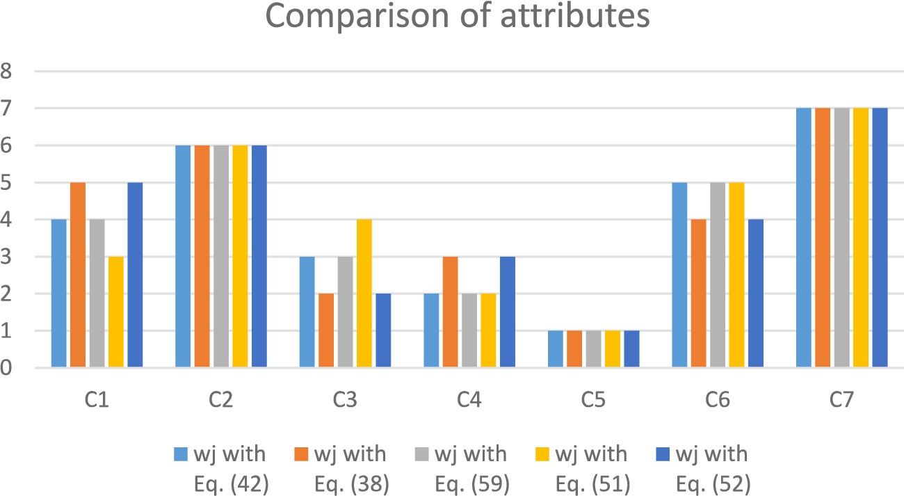
In terms of entropy-based comparison, the weight sets are determined. Table 8 gives the results of the comparison of weights and Table 9 shows the rankings of the alternatives. The entropy measures used are represented on the columns. The last two are the novel entropy measures proposed in the study and the first three are the existing ones in the literature: Eq. (44) defined by Wang et al. (2018), Eq. (48) defined by Joshi (2020a), and the knowledge measure in Eq. (52) defined by Lin et al. (2020). The third one provides a knowledge measure which is based on entropy measure and hesitancy degrees. The stepwise methodology is summarized as follows:
(a) The entropy matrix showing the entropies for each pair of alternative and attribute is derived as follows:
where(64)
(b) The knowledge matrix is derived as follows:
where(65)
Fig. 1
Comparison of the ranks of the attributes.
(c) If the knowledge measure of a criterion is larger across the alternative, it means that the value of this criterion has a smaller variation. Hence, this one shows a greater impact on the overall ratings of the alternatives. From this understanding, Eq. (66) is used for attribute weighting:
(66)
The importance ranking of the attributes is presented in Fig. 1. It is seen that there are few differences among the weight sets. Throughout the five sets, while
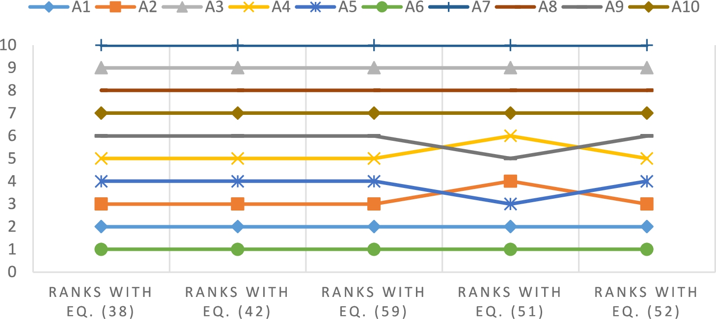
Fig. 2
Comparison of the ranks of alternatives for different weight sets.
The second analysis aims to compare the rankings of the alternatives of various approaches. Traditional CODAS developed by Keshavraz Ghorabaee et al. (2016), spherical fuzzy version of CODAS developed by Kutlu Gündoğdu and Kahraman (2019b), and spherical fuzzy extension of TOPSIS (Technique for Order Preference by Similarity to an Ideal Solution) developed by Kutlu Gündoğdu (2020) are utilized for this purpose. Each method is performed by considering two entropy measure propositions of the study, separately. To keep the flow of the study, the details of the methods are not given. The interested readers can look at the referred studies.
Fig. 3
Comparison of the ranks of alternatives for CODAS and TOPSIS versions.
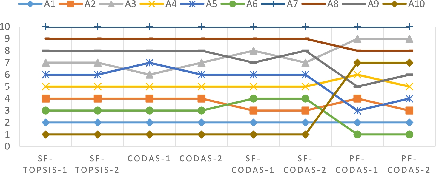
Fig. 3 shows the results of the comparisons. SF-TOPSIS, CODAS, and SF-CODAS give slightly different results while the proposed PF-CODAS generates different rankings of the alternatives. In terms of
Fig. 4
A comprehensive comparison.
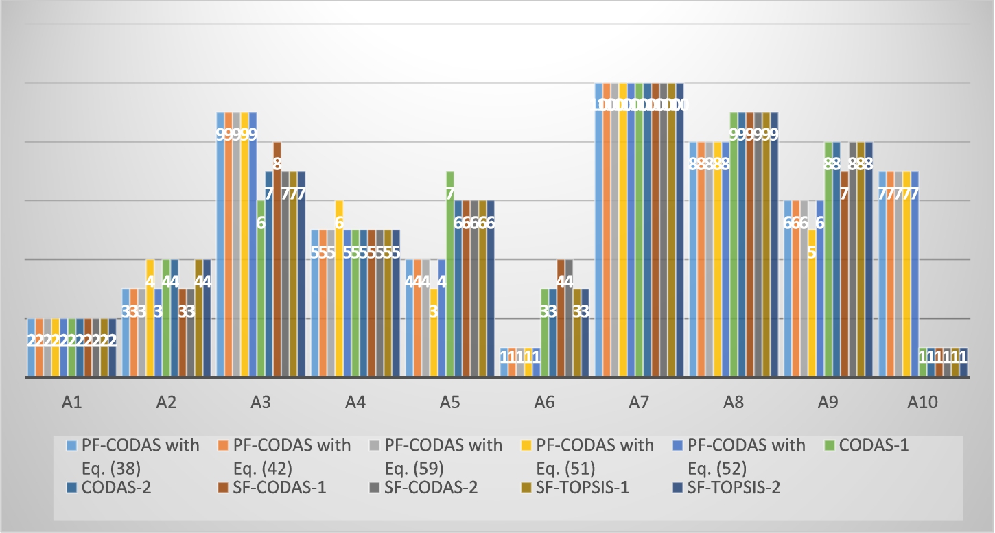
As Fig. 4 indicates, the most rank fluctuating alternatives are
For a deeper understanding of the differences generated by the proposed entropy-based SF-CODAS, Spearman’s rank correlation coefficients are also computed. Kahraman et al. (2009) proposed the usage of this statistical tool for revealing the differences between the rankings of various methods under group environment. Eq. (67) shows Spearman’s rank correlation coefficient. A larger coefficient indicates a larger level of consensus among the results of the compared approaches.
(67)
Table 10 shows the sum of the squared differences among the ranking results of CODAS and TOPSIS versions and PF-CODAS method while Table 11 shows the correlation coefficients of ρ. Except for 2 comparisons [CODAS-1 & PF-CODAS with Eq. (57) and SF-CODAS-2 & PF-CODAS with Eq. (57)], ρ coefficients are higher than 0.60. For this case, it is concluded that there are medium to high level positive correlations among the rankings of the methods used.
Table 10
Sum of the squared differences between methods.
| PF-CODAS with Eq. (44) | PF-CODAS with Eq. (48) | PF-CODAS with Eq. (66) | PF-CODAS with Eq. (57) | PF-CODAS with Eq. (58) | |
| CODAS-1 | 64 | 64 | 64 | 76 | 64 |
| CODAS-2 | 54 | 54 | 54 | 64 | 54 |
| SF-CODAS-1 | 52 | 52 | 52 | 62 | 52 |
| SF-CODAS-2 | 58 | 58 | 58 | 70 | 58 |
| SF-TOPSIS-1 | 54 | 54 | 54 | 64 | 54 |
| SF-TOPSIS-2 | 54 | 54 | 54 | 64 | 54 |
Table 11
Spearman rank correlation coefficients between methods.
| PF-CODAS with Eq. (44) | PF-CODAS with Eq. (48) | PF-CODAS with Eq. (66) | PF-CODAS with Eq. (57) | PF-CODAS with Eq. (58) | |
| CODAS-1 | 0.612 | 0.612 | 0.612 | 0.539 | 0.612 |
| CODAS-2 | 0.673 | 0.673 | 0.673 | 0.612 | 0.673 |
| SF-CODAS-1 | 0.685 | 0.685 | 0.685 | 0.624 | 0.685 |
| SF-CODAS-2 | 0.648 | 0.648 | 0.648 | 0.576 | 0.648 |
| SF-TOPSIS-1 | 0.673 | 0.673 | 0.673 | 0.612 | 0.673 |
| SF-TOPSIS-2 | 0.673 | 0.673 | 0.673 | 0.612 | 0.673 |
7Concluding Remarks
PFS has been recently accepted by the MADM domain as one of the useful fuzzy environments because of its extensive representation power of the preferences and opinions of decision-makers. PFS is defined by four elements, namely positive, negative, neutral, and refusal membership degrees and the first three elements can be independently assignable. The only rule that must be satisfied is that the sum of these four elements should be equal to 1.
Entropy is a very important information measure of fuzzy sets such as distance, inclusion, or similarity. In the literature, there are few entropy measures developed for PFSs. Entropy measures are exploited for determining the objective weights of attributes or the importance of decision-makers. These objective weights are found beneficial in case the subjective evaluation of weights is not desired or needed. The contributions of the study may be listed as follows:
• Two novel entropy measures for PFSs are developed and their proofs are given.
• CODAS, which is based on two different distance measures from the negative-ideal solution such as Euclidean and Hamming distance, is extended into PFS for the first time in the literature. Although spherical fuzzy and neutrosophic versions of CODAS can handle the hesitancy degree of the decision-makers, none of the current versions of CODAS are capable of handling their refusal degrees. The most powerful aspect of the novel extension is the simultaneous consideration of both the hesitancy and refusal degrees of the decision-makers.
• To validate the novel PF-CODAS, a real green supplier selection application for the beef industry is conducted. The rankings are compared with different applications’ rankings such as SF-TOPSIS, CODAS, and SF-CODAS. It is found that the proposed method generates different rankings of the alternatives due to the consideration of refusal degree.
• To understand the meaning of the differences in alternative rankings better, Spearman’s rank correlation coefficient is used, and it is seen that there are medium to high correlations among the alternative ranking results of the methods compared in the study. In future applications, this situation should be investigated deeply.
In the proposed method, there are some limitations that should be handled. To cope with the disadvantageous parts of the study, the possible improvements are listed as follows:
• Rather than enforcing the decision-makers to use a fixed and not-flexible linguistic term set that has PFN correspondences, a future study may work on allowing the decision-makers to directly allocate positive, neutral, and negative membership degrees so that the data collection process becomes more realistic.
• Further studies should investigate the reason behind the finding of generating different rankings of alternatives by PF-based MADM methods. In order to make more comprehensive comparisons, novel fuzzy set definitions such as Fermatean fuzzy sets (Senapati and Yager, 2020), diophantine fuzzy sets (Riaz and Hashmi, 2019), and bipolar soft sets (Mahmood, 2020) may be utilized.
• The entropy-based attribute weighting technique has some drawbacks. In some cases requiring expert opinions about the importance of attributes, subjective and objective methods can be incorporated. In this manner, the subjectivity can be kept in control while respecting the expertise of the decision-makers.
• In the literature, a few studies (Wang, 2009; Han and Xiao, 2009) criticized the entropy definitions from a probability perspective and claimed that entropy measure is not enough to measure information in a data set. To deal with these sorts of problems, future works can focus on studying newer objective attribute weighting methods, such as MEREC, SECA, CRITIC, maximizing standard deviation, etc. under picture fuzzy environment.
Table A1
The literature on fuzzy extensions of CODAS and their applications.
| Paper | CODAS Version | Hybrid Method(s) | Application |
| Keshavarz-Ghorabaee et al. (2017) | Fuzzy sets | F-EDAS and F-TOPSIS for comparison | Numerical example on market segment evaluation |
| Panchal et al. (2017) | Fuzzy sets | F-AHP for attribute weighting | Selection of an optimal maintenance strategy for an Ammonia Synthesis Unit of a urea fertilizer industry located in North India |
| Peng and Garg (2018) | Interval-valued fuzzy soft sets | IVFS-MABAC and IVFS-WDBA for comparison | A numerical example of emergency decision-making issue of mine accidents |
| Karaşan et al. (2019c) | Interval-valued hesitant fuzzy sets | F-CODAS and HF-TOPSIS for comparison | Residential construction site selection |
| Büyüközkan and Göçer (2019) | Intuitionistic fuzzy sets | IF-TOPSIS and IF-VIKOR for comparison | Prioritization of the strategies for smart city logistics |
| Karagöz et al. (2020) | Intuitionistic fuzzy sets | IF-WASPAS and IF-TOPSIS for comparison | Locating an authorized dismantling centre in Turkey |
| Dahooei et al. (2018) | Interval-valued intuitionistic fuzzy sets | IVIF-TODIM, IVIF-COPRAS, IVIF-MABAC for comparison | Evaluation of business intelligence for enterprise systems |
| Bolturk and Kahraman (2018) | Interval-valued intuitionistic fuzzy sets | CODAS for comparison | Evaluation of wave energy technology investments in Turkey |
| Roy et al. (2019) | Interval-valued intuitionistic fuzzy sets | The linear programming model for attribute weighting CODAS, F-CODAS, IVIF-VIKOR, IVIF-TOPSIS for comparison | Numerical example on an automotive parts factory in India searching for the best material for the automotive instrument panel |
| Yeni and Özçelik (2019) | Interval-valued intuitionistic fuzzy sets | IVIF-TOPSIS, IVIF-VIKOR, IVIF-SAW for comparison | Personnel selection for an engineering position in a company |
| Dahooei et al. (2020) | Interval-valued intuitionistic fuzzy sets | – | Choosing the appropriate system for cloud computing implementation in Iran |
| Deveci et al. (2020) | Interval-valued intuitionistic fuzzy sets | – | Evaluation of renewable energy alternatives in Turkey |
| Ouhibi and Frikha (2020) | Interval-valued intuitionistic fuzzy sets | – | Sorting of natural resources in Tunisia |
| Remadi and Frikha (2020) | Triangular interval-valued intuitionistic fuzzy sets | TOPSIS, VIKOR, GRA, and CODAS for comparison | Green supplier selection problem for olive oil |
| Seker and Aydin (2020) | Interval-valued intuitionistic fuzzy sets | IVIF-AHP for attribute weighting AHP&CODAS, F-AHP&F-CODAS for comparison | Determination of the most appropriate public transportation system to transfer people along the campus |
| Yalçın and Yapıcı Pehlivan (2019) | Hesitant fuzzy linguistic term sets | F-EDAS, F-TOPSIS, F-WASPAS, F-ARAS, F-COPRAS for comparison | Blue-collar personnel selection problem for a manufacturing firm in Turkey |
| Sansabas-Villalpando et al. (2019) | Hesitant fuzzy linguistic term sets | AHP for attribute weighting | Appraisal of the organizational culture of innovation and complex technological changing environments |
| Mukul et al. (2020) | Hesitant fuzzy linguistic term sets | HFL-AHP for attribute weighting | Evaluation of smart health technologies |
| Büyüközkan and Mukul (2020) | Hesitant fuzzy linguistic term sets | HFL-AHP for attribute weighting HFL-TOPSIS for comparison | Evaluation of smart health technologies |
| Bolturk (2018) | Pythagorean fuzzy sets | CODAS for comparison | Supplier selection in a manufacturing firm |
| Peng and Ma (2020) | Pythagorean fuzzy sets | TOPSIS and TODIM for comparison | Several hypothetical examples |
| Büyüközkan and Göçer (2020) | Pythagorean fuzzy sets | – | Selection of additive manufacturing technologies for the needs of the supply chain in Turkey |
| Bolturk and Kahraman (2019) | Interval-valued Pythagorean fuzzy sets | – | Selection of the best AS/RS technology |
| Peng and Li (2019) | Hesitant fuzzy soft sets | HFS-WDBA | A numerical example of an emergency decision-making issue of mine accidents |
| Wang et al. (2020) | 2-tuple linguistic neutrosophic sets | – | A numerical example for the safety assessment of a construction project |
| He et al. (2020) | 2-tuple linguistic Pythagorean fuzzy sets | 2TLPF-TODIM for comparison | Numerical example on the assessment of financial management performance |
| Karaşan et al. (2019a) | Neutrosophic sets | IVIF-TOPSIS for comparison | Wind energy plant location selection problem |
| Karaşan et al. (2019b) | Neutrosophic sets | – | Assessment of livability index of urban districts in Turkey |
| Karaşan et al. (2020) | Neutrosophic sets | – | Evaluation of defense strategies for Turkey |
| Kutlu Gündoğdu and Kahraman (2019b) | Spherical fuzzy sets | IF-TOPSIS and IF-CODAS for comparison | A hypothetical example |
| Kutlu Gündoğdu and Kahraman (2020) | Spherical fuzzy sets | IF-TOPSIS for comparison | Warehouse site selection problem |
| Karaşan et al. (2021) | Spherical fuzzy sets | – | Assessment of livability index of suburban districts in Turkey |
Appendices
A
AAppendix
Table A2
Linguistic evaluations of the decision-makers.
| VG | VG | VG | MP | MP | MP | VG | VG | VG | G | G | G | G | VG | VG | MP | F | MG | F | F | F | |
| F | MG | F | G | G | G | F | F | F | MG | G | VG | VG | VG | VG | G | MG | F | F | F | MP | |
| P | MG | G | P | MP | F | MG | G | VG | MG | MG | MG | G | MG | F | MG | MG | MG | P | MP | F | |
| MG | MG | MG | F | F | F | VG | G | MG | P | P | P | VG | G | VG | VG | G | VG | MP | F | MP | |
| F | MG | VG | VG | VG | VG | VG | G | G | P | P | MP | VP | P | MP | G | G | G | F | F | P | |
| G | G | G | F | MP | P | G | G | G | G | G | G | VG | VG | VG | F | MG | G | F | MP | F | |
| MP | F | G | MP | MP | MP | MP | F | MG | P | MP | F | P | P | MP | MP | F | MG | F | MP | F | |
| P | VG | VG | G | MG | F | F | MG | G | P | MP | F | P | P | P | VG | G | MG | F | MP | F | |
| P | MG | F | F | MP | P | MP | F | MG | MG | G | VG | MG | MG | MG | F | F | F | F | F | F | |
| MG | MG | G | MP | F | MG | MG | MG | MG | VG | VG | VG | VG | VG | VG | VG | VG | VG | P | F | F | |
Table A3
The experts’ decision matrices including PFNs.
| 0.9 | 0 | 0.05 | 0.3 | 0 | 0.6 | 0.9 | 0 | 0.05 | 0.75 | 0.05 | 0.1 | 0.75 | 0.05 | 0.1 | 0.3 | 0 | 0.6 | 0.5 | 0.1 | 0.4 | |
| 0.5 | 0.1 | 0.4 | 0.75 | 0.05 | 0.1 | 0.5 | 0.1 | 0.4 | 0.6 | 0 | 0.3 | 0.9 | 0 | 0.05 | 0.75 | 0.05 | 0.1 | 0.5 | 0.1 | 0.4 | |
| 0.25 | 0.05 | 0.6 | 0.25 | 0.05 | 0.6 | 0.6 | 0 | 0.3 | 0.6 | 0 | 0.3 | 0.75 | 0.05 | 0.1 | 0.6 | 0 | 0.3 | 0.25 | 0.05 | 0.6 | |
| 0.6 | 0 | 0.3 | 0.5 | 0.1 | 0.4 | 0.9 | 0 | 0.05 | 0.25 | 0.05 | 0.6 | 0.9 | 0 | 0.05 | 0.9 | 0 | 0.05 | 0.3 | 0 | 0.6 | |
| 0.5 | 0.1 | 0.4 | 0.9 | 0 | 0.05 | 0.9 | 0 | 0.05 | 0.25 | 0.05 | 0.6 | 0.1 | 0 | 0.85 | 0.75 | 0.05 | 0.1 | 0.5 | 0.1 | 0.4 | |
| 0.75 | 0.05 | 0.1 | 0.5 | 0.1 | 0.4 | 0.75 | 0.05 | 0.1 | 0.75 | 0.05 | 0.1 | 0.9 | 0 | 0.05 | 0.5 | 0.1 | 0.4 | 0.5 | 0.1 | 0.4 | |
| 0.3 | 0 | 0.6 | 0.3 | 0 | 0.6 | 0.3 | 0 | 0.6 | 0.25 | 0.05 | 0.6 | 0.25 | 0.05 | 0.6 | 0.3 | 0 | 0.6 | 0.5 | 0.1 | 0.4 | |
| 0.25 | 0.05 | 0.6 | 0.75 | 0.05 | 0.1 | 0.5 | 0.1 | 0.4 | 0.25 | 0.05 | 0.6 | 0.25 | 0.05 | 0.6 | 0.9 | 0 | 0.05 | 0.5 | 0.1 | 0.4 | |
| 0.25 | 0.05 | 0.6 | 0.5 | 0.1 | 0.4 | 0.3 | 0 | 0.6 | 0.6 | 0 | 0.3 | 0.6 | 0 | 0.3 | 0.5 | 0.1 | 0.4 | 0.5 | 0.1 | 0.4 | |
| 0.6 | 0 | 0.3 | 0.3 | 0 | 0.6 | 0.6 | 0 | 0.3 | 0.9 | 0 | 0.05 | 0.9 | 0 | 0.05 | 0.9 | 0 | 0.05 | 0.25 | 0.05 | 0.6 | |
| 0.9 | 0 | 0.05 | 0.3 | 0 | 0.6 | 0.9 | 0 | 0.05 | 0.75 | 0.05 | 0.1 | 0.9 | 0 | 0.05 | 0.5 | 0.1 | 0.4 | 0.5 | 0.1 | 0.4 | |
| 0.6 | 0 | 0.3 | 0.75 | 0.05 | 0.1 | 0.5 | 0.1 | 0.4 | 0.75 | 0.05 | 0.1 | 0.9 | 0 | 0.05 | 0.6 | 0 | 0.3 | 0.5 | 0.1 | 0.4 | |
| 0.6 | 0 | 0.3 | 0.3 | 0 | 0.6 | 0.75 | 0.05 | 0.1 | 0.6 | 0 | 0.3 | 0.6 | 0 | 0.3 | 0.6 | 0 | 0.3 | 0.3 | 0 | 0.6 | |
| 0.6 | 0 | 0.3 | 0.5 | 0.1 | 0.4 | 0.75 | 0.05 | 0.1 | 0.25 | 0.05 | 0.6 | 0.75 | 0.05 | 0.1 | 0.75 | 0.05 | 0.1 | 0.5 | 0.1 | 0.4 | |
| 0.6 | 0 | 0.3 | 0.9 | 0 | 0.05 | 0.75 | 0.05 | 0.1 | 0.25 | 0.05 | 0.6 | 0.25 | 0.05 | 0.6 | 0.75 | 0.05 | 0.1 | 0.5 | 0.1 | 0.4 | |
| 0.75 | 0.05 | 0.1 | 0.3 | 0 | 0.6 | 0.75 | 0.05 | 0.1 | 0.75 | 0.05 | 0.1 | 0.9 | 0 | 0.05 | 0.6 | 0 | 0.3 | 0.3 | 0 | 0.6 | |
| 0.5 | 0.1 | 0.4 | 0.3 | 0 | 0.6 | 0.5 | 0.1 | 0.4 | 0.3 | 0 | 0.6 | 0.25 | 0.05 | 0.6 | 0.5 | 0.1 | 0.4 | 0.3 | 0 | 0.6 | |
| 0.9 | 0 | 0.05 | 0.6 | 0 | 0.3 | 0.6 | 0 | 0.3 | 0.3 | 0 | 0.6 | 0.25 | 0.05 | 0.6 | 0.75 | 0.05 | 0.1 | 0.3 | 0 | 0.6 | |
| 0.6 | 0 | 0.3 | 0.3 | 0 | 0.6 | 0.5 | 0.1 | 0.4 | 0.75 | 0.05 | 0.1 | 0.6 | 0 | 0.3 | 0.5 | 0.1 | 0.4 | 0.5 | 0.1 | 0.4 | |
| 0.6 | 0 | 0.3 | 0.5 | 0.1 | 0.4 | 0.6 | 0 | 0.3 | 0.9 | 0 | 0.05 | 0.9 | 0 | 0.05 | 0.9 | 0 | 0.05 | 0.5 | 0.1 | 0.4 | |
| 0.9 | 0 | 0.05 | 0.3 | 0 | 0.6 | 0.9 | 0 | 0.05 | 0.75 | 0.05 | 0.1 | 0.9 | 0 | 0.05 | 0.6 | 0 | 0.3 | 0.5 | 0.1 | 0.4 | |
| 0.5 | 0.1 | 0.4 | 0.75 | 0.05 | 0.1 | 0.5 | 0.1 | 0.4 | 0.9 | 0 | 0.05 | 0.9 | 0 | 0.05 | 0.5 | 0.1 | 0.4 | 0.3 | 0 | 0.6 | |
| 0.75 | 0.05 | 0.1 | 0.5 | 0.1 | 0.4 | 0.9 | 0 | 0.05 | 0.6 | 0 | 0.3 | 0.5 | 0.1 | 0.4 | 0.6 | 0 | 0.3 | 0.5 | 0.1 | 0.4 | |
| 0.6 | 0 | 0.3 | 0.5 | 0.1 | 0.4 | 0.6 | 0 | 0.3 | 0.25 | 0.05 | 0.6 | 0.9 | 0 | 0.05 | 0.9 | 0 | 0.05 | 0.3 | 0 | 0.6 | |
| 0.9 | 0 | 0.05 | 0.9 | 0 | 0.05 | 0.75 | 0.05 | 0.1 | 0.3 | 0 | 0.6 | 0.3 | 0 | 0.6 | 0.75 | 0.05 | 0.1 | 0.25 | 0.05 | 0.6 | |
| 0.75 | 0.05 | 0.1 | 0.25 | 0.05 | 0.6 | 0.75 | 0.05 | 0.1 | 0.75 | 0.05 | 0.1 | 0.9 | 0 | 0.05 | 0.75 | 0.05 | 0.1 | 0.5 | 0.1 | 0.4 | |
| 0.75 | 0.05 | 0.1 | 0.3 | 0 | 0.6 | 0.6 | 0 | 0.3 | 0.5 | 0.1 | 0.4 | 0.3 | 0 | 0.6 | 0.6 | 0 | 0.3 | 0.5 | 0.1 | 0.4 | |
| 0.9 | 0 | 0.05 | 0.5 | 0.1 | 0.4 | 0.75 | 0.05 | 0.1 | 0.5 | 0.1 | 0.4 | 0.25 | 0.05 | 0.6 | 0.6 | 0 | 0.3 | 0.5 | 0.1 | 0.4 | |
| 0.5 | 0.1 | 0.4 | 0.25 | 0.05 | 0.6 | 0.6 | 0 | 0.3 | 0.9 | 0 | 0.05 | 0.6 | 0 | 0.3 | 0.5 | 0.1 | 0.4 | 0.5 | 0.1 | 0.4 | |
| 0.75 | 0.05 | 0.1 | 0.6 | 0 | 0.3 | 0.6 | 0 | 0.3 | 0.9 | 0 | 0.05 | 0.9 | 0 | 0.05 | 0.9 | 0 | 0.05 | 0.5 | 0.1 | 0.4 | |
Table A4
The weighted normalized picture fuzzy decision matrix for Eq. (58).
| 0.282 | 0.000 | 0.650 | 0.046 | 0.000 | 0.934 | 0.292 | 0.000 | 0.638 | 0.185 | 0.642 | 0.113 | 0.288 | 0.000 | 0.627 | 0.093 | 0.000 | 0.878 | 0.055 | 0.775 | 0.170 | |
| 0.106 | 0.000 | 0.862 | 0.169 | 0.671 | 0.106 | 0.099 | 0.708 | 0.193 | 0.201 | 0.000 | 0.724 | 0.320 | 0.000 | 0.606 | 0.136 | 0.000 | 0.808 | 0.064 | 0.000 | 0.915 | |
| 0.117 | 0.000 | 0.826 | 0.057 | 0.000 | 0.919 | 0.204 | 0.000 | 0.721 | 0.127 | 0.000 | 0.837 | 0.153 | 0.000 | 0.785 | 0.126 | 0.000 | 0.837 | 0.080 | 0.000 | 0.892 | |
| 0.123 | 0.000 | 0.841 | 0.088 | 0.736 | 0.176 | 0.204 | 0.000 | 0.721 | 0.042 | 0.642 | 0.296 | 0.277 | 0.000 | 0.634 | 0.248 | 0.000 | 0.670 | 0.076 | 0.000 | 0.901 | |
| 0.166 | 0.000 | 0.788 | 0.264 | 0.000 | 0.671 | 0.220 | 0.000 | 0.686 | 0.045 | 0.000 | 0.927 | 0.042 | 0.000 | 0.934 | 0.185 | 0.643 | 0.113 | 0.064 | 0.758 | 0.172 | |
| 0.181 | 0.650 | 0.111 | 0.057 | 0.000 | 0.919 | 0.188 | 0.638 | 0.114 | 0.185 | 0.642 | 0.113 | 0.320 | 0.000 | 0.606 | 0.136 | 0.000 | 0.808 | 0.068 | 0.000 | 0.910 | |
| 0.109 | 0.000 | 0.840 | 0.046 | 0.000 | 0.934 | 0.094 | 0.000 | 0.876 | 0.063 | 0.000 | 0.911 | 0.050 | 0.000 | 0.918 | 0.093 | 0.000 | 0.878 | 0.068 | 0.000 | 0.910 | |
| 0.217 | 0.000 | 0.724 | 0.124 | 0.000 | 0.825 | 0.138 | 0.000 | 0.805 | 0.063 | 0.000 | 0.911 | 0.047 | 0.606 | 0.325 | 0.201 | 0.000 | 0.725 | 0.068 | 0.000 | 0.910 | |
| 0.091 | 0.000 | 0.877 | 0.057 | 0.000 | 0.919 | 0.094 | 0.000 | 0.876 | 0.201 | 0.000 | 0.724 | 0.142 | 0.000 | 0.817 | 0.097 | 0.712 | 0.191 | 0.055 | 0.775 | 0.170 | |
| 0.141 | 0.000 | 0.802 | 0.084 | 0.000 | 0.889 | 0.128 | 0.000 | 0.835 | 0.288 | 0.000 | 0.642 | 0.320 | 0.000 | 0.606 | 0.288 | 0.000 | 0.643 | 0.064 | 0.758 | 0.172 | |
| 0.091 | 0.000 | 0.877 | 0.046 | 0.000 | 0.934 | 0.094 | 0.000 | 0.876 | 0.042 | 0.000 | 0.927 | 0.042 | 0.000 | 0.934 | 0.093 | 0.000 | 0.878 | 0.055 | 0.000 | 0.915 | |
Table A5
Euclidean and Hamming distances to the negative-ideal solution for Eq. (58).
| 0.608 | 0.647 | |
| 0.583 | 0.592 | |
| 0.116 | 0.132 | |
| 0.558 | 0.583 | |
| 0.575 | 0.568 | |
| 0.687 | 0.766 | |
| 0.020 | 0.019 | |
| 0.346 | 0.303 | |
| 0.564 | 0.504 | |
| 0.472 | 0.480 |
Table A6
Comparison of distances and the ranking of alternatives for Eq. (58).
| Rank | ||||||||||||
| 0.000 | 0.025 | 1.007 | 0.115 | 0.033 | −0.079 | 1.216 | 0.606 | 0.044 | 0.302 | 3.271 | 2 | |
| −0.025 | 0.000 | 0.926 | 0.025 | 0.008 | −0.104 | 1.135 | 0.526 | 0.019 | 0.222 | 2.731 | 3 | |
| −0.493 | −0.467 | 0.000 | −0.442 | −0.459 | −0.571 | 0.208 | −0.230 | −0.448 | −0.357 | −3.260 | 9 | |
| −0.050 | −0.025 | 0.893 | 0.000 | −0.017 | −0.129 | 1.101 | 0.492 | −0.006 | 0.188 | 2.447 | 5 | |
| −0.033 | −0.008 | 0.895 | 0.017 | 0.000 | −0.112 | 1.103 | 0.494 | 0.011 | 0.190 | 2.558 | 4 | |
| 0.198 | 0.279 | 1.205 | 0.312 | 0.310 | 0.000 | 1.413 | 0.804 | 0.385 | 0.500 | 5.406 | 1 | |
| −0.588 | −0.562 | −0.095 | −0.538 | −0.555 | −0.666 | 0.000 | −0.326 | −0.544 | −0.452 | −4.326 | 10 | |
| −0.262 | −0.237 | 0.401 | −0.212 | −0.229 | −0.341 | 0.609 | 0.000 | −0.218 | −0.126 | −0.615 | 8 | |
| −0.044 | −0.019 | 0.820 | 0.006 | −0.011 | −0.123 | 1.028 | 0.419 | 0.000 | 0.115 | 2.192 | 6 | |
| −0.136 | −0.111 | 0.705 | −0.086 | −0.103 | −0.215 | 0.913 | 0.304 | −0.092 | 0.000 | 1.180 | 7 |
References
1 | Arya, V., Kumar, S. ((2020) a). A new picture fuzzy information measure based on shannon entropy with applications in opinion polls using extended VIKOR–TODIM approach. Computational and Applied Mathematics, 39: , 197. |
2 | Arya, V., Kumar, S. ((2020) b). A novel TODIM-VIKOR approach based on entropy and Jensen–Tsalli divergence measure for picture fuzzy sets in a decision-making problem. International Journal of Intelligent Systems, 35: (12), 2140–2180. |
3 | Atanassov, K.T. ((1986) ). Intuitionistic fuzzy sets. Fuzzy Sets and Systems, 20: , 87–96. |
4 | Aydoğdu, A. ((2020) ). Subsethood measure for picture fuzzy sets. In: Proceedings of International Marmara Sciences Congress (Spring), Kocaeli, Turkey, June 19–20, pp. 557–562. |
5 | Aydoğdu, A., Gül, S. ((2020) ). A novel entropy proposition for spherical fuzzy sets and its application in multiple attribute decision-making. International Journal of Intelligent Systems, 35: (9), 1354–1374. |
6 | Bolturk, E. ((2018) ). Pythagorean fuzzy CODAS and its application to supplier selection in a manufacturing firm. Journal of Enterprise Information Management, 31: (4), 550–564. |
7 | Bolturk, E., Kahraman, C. ((2018) ). Interval-valued intuitionistic fuzzy CODAS method and its application to wave energy facility location selection problem. Journal of Intelligent & Fuzzy Systems, 35: (4), 4865–4877. |
8 | Bolturk, E., Kahraman, C. ((2019) ). A modified interval-valued Pythagorean fuzzy CODAS method and evaluation of AS/RS technologies. Journal of Multiple-Valued Logic and Soft Computing, 33: (4–5), 415–429. |
9 | Büyüközkan, G., Çifçi, G. ((2012) ). A novel hybrid MCDM approach based on fuzzy DEMATEL, fuzzy ANP and fuzzy TOPSIS to evaluate green suppliers. Expert Systems with Applications, 39: , 3000–3011. |
10 | Büyüközkan, G., Göçer, F. ((2019) ). Prioritizing the strategies to enhance Smart city logistics by intuitionistic fuzzy CODAS. In: Proceeding of the 11th Conference of the European Society for Fuzzy Logic and Technology, September 9–13. Prague, Czech Republic. |
11 | Büyüközkan, G., Göçer, F. ((2020) ). Assessment of additive manufacturing technology by pythagorean fuzzy CODAS. In: Kahraman, C., Cebi, S., Cevik Onar, S., Oztaysi, B., Tolga, A., Sari, I. (Eds.), Intelligent and Fuzzy Techniques in Big Data Analytics and Decision Making. Advances in Intelligent Systems and Computing, Vol. 1029: . Springer Nature, Switzerland, pp. 959–968. |
12 | Büyüközkan, G., Mukul, E. ((2020) ). Evaluation of smart health technologies with hesitant fuzzy linguistic MCDM methods. Journal of Intelligent & Fuzzy Systems, 39: (5), 6363–6375. |
13 | Cuong, B.C. ((2014) ). Picture fuzzy sets. Journal of Computer Science and Cybernetics, 30: (4), 409–420. |
14 | Cuong, B.C., Kreinovich, V. ((2013) ). Picture Fuzzy Sets – a new concept for computational intelligence problems. In: Proceeding of the 3rd World Congress on Information and Communication Technologies, December 15-18. Hanoi, Vietnam, pp. 1–6. |
15 | Çalık, A. ((2021) ). A novel Pythagorean fuzzy AHP and fuzzy TOPSIS methodology for green supplier selection in the Industry 4.0 era. Soft Computing, 25: , 2253–2265. |
16 | Çalışkan, H., Kurşuncu, B., Kurbanoğlu, C., Güven, Ş.Y. ((2013) ). Material selection for the tool holder working under hard milling conditions using different multi criteria decision making methods. Materials and Design, 45: , 473–479. |
17 | Dahooei, J.H., Zavadskas, E.K., Vanaki, A.S., Firoozfar, H.R., Keshavarz-Ghorabaee, M. ((2018) ). An evaluation model of business intelligence for enterprise systems with new extension of codas (CODAS-IVIF). Information Management, 3: (XXI), 171–187. |
18 | Dahooei, J.H., Vanaki, A.S., Mohammadi, N. ((2020) ). Choosing the appropriate system for cloud computing implementation by using the interval-valued intuitionistic fuzzy CODAS multiattribute decision-making method (Case study: Faculty of New Sciences and Technologies of Tehran University). IEEE Transactions on Engineering Management, 67: (3), 855–868. |
19 | Deveci, K., Cin, R., Kağızman, A. ((2020) ). A modified interval valued intuitionistic fuzzy CODAS method and its application to multi-criteria selection among renewable energy alternatives in Turkey. Applied Soft Computing Journal, 96: , 106660. |
20 | Dinh, V.N., Thao, N.X. ((2018) ). Some measures of picture fuzzy sets and their application in multi-attribute decision making. International Journal of Mathematical Sciences and Computing, 3: , 23–41. |
21 | Dutta, P. ((2018) ). Medical diagnosis based on distance measures between picture fuzzy sets. International Journal of Fuzzy System Applications, 7: (4), 15–36. |
22 | Freeman, J., Chen, T. ((2015) ). Green supplier selection using an AHP-Entropy-TOPSIS framework. Supply Chain Management: An International Journal, 20: (3), 327–340. |
23 | Govindan, K., Rajendran, S., Sarkis, J., Murugesan, P. ((2015) ). Multi criteria decision making approaches for green supplier evaluation and selection: a literature review. Journal of Cleaner Production, 98: , 66–83. |
24 | Han, R.C., Xiao, J.X. ((2009) ). Deciding weighing by entropy value method is an error. In: Proceedings of Second International Conference on Information and Computing Science, May 21–22. Manchester, UK, pp. 255–257. |
25 | He, T., Zhang, S., Wei, G., Wang, R., Wu, J., Wei, C. ((2020) ). CODAS method for 2-tuple linguistic pythagorean fuzzy multiple attribute group decision making and its application to financial management performance assessment. Technological and Economic Development of Economy, 26: (4), 920–932. |
26 | Joshi, R. ((2020) a). A new picture fuzzy information measure based on Tsallis–Havrda–Charvat concept with applications in presaging poll outcome. Computational and Applied Mathematics, 39: , 71. |
27 | Joshi, R. ((2020) b). A novel decision-making method using R-Norm concept and VIKOR approach under picture fuzzy environment. Expert Systems with Applications, 147: , 113228. |
28 | Kabak, Ö., Ruan, D. ((2011) ). A comparison study of fuzzy MADM methods in nuclear safeguards evaluation. Journal of Global Optimization, 51: , 209–226. |
29 | Kahraman, C., Engin, O., Kabak, Ö., Kaya, İ. ((2009) ). Information systems outsourcing decisions using a group decision-making approach. Engineering Applications of Artificial Intelligence, 22: , 832–841. |
30 | Karagöz, S., Deveci, M., Simic, V., Aydin, N., Bolukbas, U. ((2020) ). A novel intuitionistic fuzzy MCDM-based CODAS approach for locating an authorized dismantling center: a case study of Istanbul. Waste Management & Research: The Journal for a Sustainable Circular Economy, 38: (6), 660–672. |
31 | Karaşan, A., Boltürk, E., Kahraman, C. ((2019) a). A novel neutrosophic CODAS method: selection among wind energy plant locations. Journal of Intelligent & Fuzzy Systems, 36: (2), 1491–1504. |
32 | Karaşan, A., Boltürk, E., Kahraman, C. ((2019) b). An integrated methodology using neutrosophic CODAS & fuzzy inference system: assessment of livability index of urban districts. Journal of Intelligent & Fuzzy Systems, 36: (6), 5443–5455. |
33 | Karaşan, A., Zavadskas, E.K., Kahraman, C., Keshavarz Ghorabaee, M. ((2019) c). Residential construction site selection through interval-valued hesitant fuzzy CODAS method. Informatica, 30: (4), 689–710. |
34 | Karaşan, A., Kaya, İ., Erdoğan, M., Özkan, B., Çolak, M. ((2020) ). Evaluation of defense strategies by using a MCDM methodology based on neutrosophic sets: a case study for Turkey. In: Kahraman, C., Cebi, S., Cevik Onar, S., Oztaysi, B., Tolga, A., Sari, I. (Eds.), Intelligent and Fuzzy Techniques in Big Data Analytics and Decision Making. Advances in Intelligent Systems and Computing, Vol. 1029: . Springer Nature, Switzerland, pp. 683–692. |
35 | Karaşan, A., Boltürk, E., Kutlu Gündoğdu, F. ((2021) ). Assessment of livability indices of suburban places of Istanbul by using spherical fuzzy CODAS method. In: Kahraman, C., Kutlu Gündoğdu, F. (Eds.), Decision Making with Spherical Fuzzy Sets. Studies in Fuzziness and Soft Computing, Vol. 392: . Springer, Berlin, Heidelberg, pp. 277–293. |
36 | Keshavarz-Ghorabaee, M., Zavadskas, E.K., Turskis, Z., Antucheviciene, J. ((2016) ). A new combinative distance-based assessment (CODAS) method for multi-criteria decision-making. Economic Computation and Economic Cybernetics Studies and Research, 3: (50), 25–44. |
37 | Keshavarz-Ghorabaee, M., Amiri, M., Zavadskas, E.K., Hooshmand, R., Antucheviciene, J. ((2017) ). Fuzzy extension of the codas method for multi-criteria market segment evaluation. Journal of Business Economics and Management, 18: (1), 1–19. |
38 | Keshavarz-Ghorabaee, M., Amiri, M., Zavadskas, E.K., Turskis, Z., Antucheviciene, J. ((2018) ). Simultaneous evaluation of criteria and alternatives (SECA) for multi-criteria decision-making. Informatica, 29: (2), 265–280. |
39 | Keshavarz-Ghorabaee, M., Amiri, M., Zavadskas, E.K., Turskis, Z., Antucheviciene, J. ((2021) ). Determination of objective weights using a new method based on the removal effects of criteria (MEREC). Symmetry, 13: , 525. |
40 | Kumar, S., Barman, A.G. ((2021) ). Fuzzy TOPSIS and fuzzy VIKOR in selecting green suppliers for sponge iron and steel manufacturing. Soft Computing, 25: , 6505–6525. |
41 | Kutlu Gündoğdu, F. ((2020) ). Principals of spherical fuzzy sets. In: Kahraman, C., Cebi, S., Cevik Onar, S., Oztaysi, B., Tolga, A., Sari, I. (Eds.), Intelligent and Fuzzy Techniques in Big Data Analytics and Decision Making. Advances in Intelligent Systems and Computing, Vol. 1029: . Springer Nature, Switzerland, pp. 15–23. |
42 | Kutlu Gündoğdu, F., Kahraman, C. ((2019) a). Spherical fuzzy sets and spherical fuzzy TOPSIS method. Journal of Intelligent & Fuzzy Systems, 36: (1), 337–352. |
43 | Kutlu Gündoğdu, F., Kahraman, C. ((2019) b). Extension of codas with spherical fuzzy sets. Journal of Multiple-Valued Logic and Soft Computing, 33: (4–5), 481–505. |
44 | Kutlu Gündoğdu, F., Kahraman, C. ((2020) ). Spherical fuzzy sets and decision making applications. In: Kahraman, C., Cebi, S., Cevik Onar, S., Oztaysi, B., Tolga, A., Sari, I. (Eds.), Intelligent and Fuzzy Techniques in Big Data Analytics and Decision Making. Advances in Intelligent Systems and Computing, Vol. 1029: . Springer Nature, Switzerland, pp. 979–987. |
45 | Li, L., Liu, F., Li, C. ((2014) ). Customer satisfaction evaluation method for customized product development using entropy weight and analytic hierarchy process. Computers & Industrial Engineering, 77: , 80–87. |
46 | Lin, M., Huang, C., Xu, Z. ((2020) ). MULTIMOORA based MCDM model for site selection of car sharing station under picture fuzzy environment. Sustainable Cities and Society, 53: , 101873. |
47 | Liou, J.J.H., Chang, M.H., Lo, H.W., Hsu, M.H. ((2021) ). Application of an MCDM model with data mining techniques for green supplier evaluation and selection. Applied Soft Computing Journal, 109: , 107534. |
48 | Mahmood, T. (2020). A novel approach towards bipolar soft sets and their applications. Journal of Mathematics, 2020, Article ID 4690808. |
49 | Meksavang, P., Shi, H., Lin, S.M., Liu, H.C. ((2019) ). An extended picture fuzzy VIKOR approach for sustainable supplier management and its application in the beef industry. Symmetry, 11: , 468. |
50 | Mukul, E., Güler, M., Büyüközkan, G. ((2020) ). Evaluation of smart health technologies with hesitant fuzzy MCDM methods. In: Kahraman, C., Cebi, S., Cevik Onar, S., Oztaysi, B., Tolga, A., Sari, I. (Eds.), Intelligent and Fuzzy Techniques in Big Data Analytics and Decision Making. Advances in Intelligent Systems and Computing, Vol. 1029: . Springer Nature, Switzerland, pp. 1059–1067. |
51 | Ouhibi, A., Frikha, H. (2020). Interval-valued intuitionistic fuzzy CODAS-SORT method: evaluation of natural resources in Tunisia. In: 2020 International Multi-Conference on: “Organization of Knowledge and Advanced Technologies” (OCTA), February 6–8, Tunis, Tunisia. |
52 | Panchal, D., Chatterjee, P., Shukla, R.K., Choudhury, T., Tamosaitiene, J. ((2017) ). Integrated fuzzy AHP-CODAS framework for maintenance decision in urea fertilizer industry. Economic Computation and Economic Cybernetics Studies and Research, 3: (51), 179–196. |
53 | Peng, X., Garg, H. ((2018) ). Algorithms for interval-valued fuzzy soft sets in emergency decision making based on WDBA and CODAS with new information measure. Computers & Industrial Engineering, 119: , 439–452. |
54 | Peng, X., Li, W. ((2019) ). Algorithms for hesitant fuzzy soft decision making based on revised aggregation operators, WDBA and CODAS. Journal of Intelligent & Fuzzy Systems, 36: (6), 6307–6323. |
55 | Peng, X., Ma, X. ((2020) ). Pythagorean fuzzy multi-criteria decision making method based on CODAS with new score function. Journal of Intelligent & Fuzzy Systems, 38: (3), 3307–3318. |
56 | Remadi, D.F., Frikha, H.M. (2020). The triangular intuitionistic fuzzy extension of the CODAS method for solving multi-criteria group decision making. In: 2020 International Multi-Conference on: “Organization of Knowledge and Advanced Technologies” (OCTA), February 6–8, Tunis, Tunisia. |
57 | Riaz, M., Hashmi, M.R. ((2019) ). Linear Diophantine fuzzy set and its applications towards multi-attribute decision-making problems. Journal of Intelligent & Fuzzy Systems, 37: (4), 5417–5439. |
58 | Roy, J., Das, S., Kar, S., Pamucar, D. ((2019) ). An extension of the CODAS approach using interval-valued intuitionistic fuzzy set for sustainable material selection in construction projects with incomplete weight information. Symmetry, 11: , 393. |
59 | Sansabas-Villalpando, V., Perez-Olguin, I.J.C., Perez-Dominguez, L.A., Rodriguez-Picon, L.A., Mendez-Gonzalez, L.C. ((2019) ). CODAS HFLTS method to appraise organizational culture of innovation and complex technological changes environments. Sustainability, 11: , 7045. |
60 | Seker, S., Aydin, N. ((2020) ). Sustainable public transportation system evaluation: a novel two-stage hybrid method based on IVIF-AHP and CODAS. International Journal of Fuzzy Systems, 22: (1), 257–272. |
61 | Senapati, T., Yager, R.R. ((2020) ). Fermatean fuzzy sets. Journal of Ambient Intelligence and Humanized Computing, 11: , 663–674. |
62 | Singh, P., Mishra, N.K., Kumar, M., Saxena, S., Singh, V. ((2018) ). Risk analysis of flood disaster based on similarity measures in picture fuzzy environment. Afrika Matematika, 29: (7–8), 1019–1038. |
63 | Smarandache, F. ((1999) ). A unifying field in logics neutrosophy: neutrosophic probability, set and logic. American Research Press, Rehoboth. |
64 | Son, L.H. ((2016) ). Generalized picture distance measure and applications to picture fuzzy clustering. Applied Soft Computing Journal, 46: , 284–295. |
65 | Thao, N.X. ((2020) ). Similarity measures of picture fuzzy sets based on entropy and their application in MCDM. Pattern Analysis and Applications, 23: (3), 1203–1213. |
66 | Wang, C., Zhou, X., Tu, H., Tao, S. ((2017) ). Some geometric aggregation operators based on picture fuzzy sets and their application in multiple attribute decision making. Italian Journal of Pure and Applied Mathematics, 37: , 477–492. |
67 | Wang, L., Zhang, H.Y., Wang, J.Q., Li, L. ((2018) ). Picture fuzzy normalized projection-based VIKOR method for the risk evaluation of construction project. Applied Soft Computing Journal, 64: , 216–226. |
68 | Wang, P., Wang, J., Wei, G., Wu, J., Wei, C., Wei, Y. ((2020) ). CODAS method for multiple attribute group decision making under 2-tuple linguistic neutrosophic environment. Informatica, 31: (1), 161–184. |
69 | Wang, Y. ((2009) ). Analyses on limitations of information theory. In: Proceedings of International Conference on Artificial Intelligence and Computational Intelligence, November 7–8. Shanghai, China, pp. 85–88. |
70 | Wei, C., Wu, J., Guo, Y., Wei, G. ((2021) ). Green supplier selection based on CODAS method in probabilistic uncertain linguistic environment. Technological and Economic Development of Economy, 27: (3), 530–549. |
71 | Wei, G. ((2017) a). Picture fuzzy aggregation operators and their application to multiple attribute decision making. Journal of Intelligent & Fuzzy Systems, 33: , 713–724. |
72 | Wei, G. ((2017) b). Some cosine similarity measures for picture fuzzy sets and their applications to strategic decision making. Informatica, 28: (3), 547–564. |
73 | Wei, G. ((2018) a). TODIM method for picture fuzzy multiple attribute decision making. Informatica, 29: (3), 555–566. |
74 | Wei, G. ((2018) b). Some similarity measures for picture fuzzy sets and their applications. Iranian Journal of Fuzzy Systems, 15: (1), 77–89. |
75 | Wei, G., Gao, H. ((2018) ). The generalized Dice similarity measures for picture fuzzy sets and their applications. Informatica, 29: (1), 107–124. |
76 | Yager, R.R. ((2013) ). Pythagorean fuzzy subsets. In: Proceedings of Joint IFSA World Congress and NAFIPS Annual Meeting, Edmonton, Canada, June 24–28, pp. 57–61. |
77 | Yager, R.R. ((2017) ). Generalized orthopair fuzzy sets. IEEE Transactions on Fuzzy Systems, 25: (5), 1222–1230. |
78 | Yalçın, N., Yapıcı Pehlivan, N. ((2019) ). Application of the fuzzy CODAS method based on fuzzy envelopes for hesitant fuzzy linguistic term sets: a case study on a personnel selection problem. Symmetry, 11: , 493. |
79 | Yeni, F.B., Özçelik, G. ((2019) ). Interval-valued Atanassov Intuitionistic fuzzy CODAS method for multi criteria group decision making problems. Group Decision and Negotiation, 28: , 433–452. |
80 | Zadeh, L.A. ((1965) ). Fuzzy sets. Information & Control, 8: , 338–353. |


