
Behavioural Representation of the Aorta by Utilizing Windkessel and Agent-Based Modelling
Abstract
The main objective of the present paper is to report two studies on mathematical and computational techniques used to model the behaviour of the aorta in the human cardiovascular system. In this paper, an account of the design and implementation of two distinct models is presented: a Windkessel model and an agent-based model. Windkessel model represents the left heart and arterial system of the cardiovascular system in the physiological domain. The agent-based model offers a simplified account of arterial behaviour by randomly generating arterial parameter values. This study has described the mechanism how and when the left heart contracts and pumps the blood out of the aorta, and it has taken the Windkessel model one step further. The results of this study show that the dynamics of the aorta can be explored in each modelling approaches as proposed and implemented by our research group. It is thought that this study will contribute to the literature in terms of development of the Windkessel model by considering its timing and redesigning it with digital electronics perspective.
1Introduction
In recent years, researchers in many areas of scientific fields, such as computer science, sociology, mathematics, physics, economics, and biology, have realized the importance of complex systems analysis, modelling, and engineering (Ma’ayan, 2017). Today, modelling approaches are essential in interdisciplinary fields, including biomedical engineering, biophysics, and system physiology, which not only require thorough knowledge of mathematical (e.g. calculus, linear algebra, and differential equations) and engineering (electronic, photonic, mechanical, and materials) skills (Northrop, 2010), but also a computer-based analysis of a system’s properties. For example, biological systems are understood to be highly complex given that they involve many subsystems, which, in turn, have a structure and organizational principles (Cardelli, 2005). Human physiology is considered a complex system inasmuch as it consists of a number of biological systems comprising a large number of interacting components such as agents and processes (Rocha, 2020). In the domain of human physiology, the cardiovascular system (CVS) is defined as a sophisticated mechanism including complex interactions and physiological processes (Kokalari et al., 2013; Guyton and Hall, 2015). In efforts to understand the physiological dynamics and complex interactions of the CVS, modelling and simulation approaches play an important role in predicting the response to external or internal conditions and in investigating system perturbations (Fischer, 2008).
In the present study, we describe some of the methods developed to model the CVS, with a focus on two distinct modelling approaches: Windkessel model and agent-based modelling and simulation (ABMS). These modelling approaches provide a foundation for understanding both the dynamics and complexity of the CVS. We improve the Windkessel model by connecting it with an astable multivibrator that provides the timing of the systole and diastole phases during the cardiac cycle and an inverter circuit to represent the aortic valve and the aorta. Based on digital electronics and including 3-element Windkessel model, the Windkessel model explains both the behaviour of the left heart and the aorta and their timing. In order to establish the relative effectiveness of our model, we constructed a digital circuit for the model with real electronic components and observed its behaviour.
Agent-based model comprises a network, a grid, and a continuous space in the Repast Simphony platform (North et al., 2007) that composes a simulated environment. In this model, we define the left heart and the blood vessel segments in the arterial system. The left heart and blood vessel segments are represented by agents, i.e. actors, in the simulated environment. The data we obtained from the simulation reflects the behaviour of real blood vessels in the aorta.
The rest of the study is organized as follows: a detailed description of the CVS is given in Section 2; a review of studies in which researchers propose models of the CVS is presented in Section 3; a description of the methods and our modelling approaches are described in Section 4; the circuit model is developed and the simulation results are given in Section 5; an account of the evaluation and a more general discussion of the study are given in Section 6; the conclusion, including a summary of the study and recommendations for future research directions, is presented in Section 7.
2Human Cardiovascular System
The human cardiovascular system (CVS) is a closed loop circulatory system in which vital functions, such as the circulation of oxygen, nutrients, hormones, ions, and fluids, and the removal of metabolic waste, are maintained. This system consists of two important circulatory processes that take place simultaneously within the body: systemic circulation and pulmonary circulation. The blood’s circulatory cycle begins with systemic circulation. The left ventricle (LV) of the heart pumps oxygen-rich blood into the main artery, i.e. the aorta. The blood travels from the aorta to the arterial branches and arterioles into the capillary bed, where it releases oxygen and nutrients and other important substances, and then continues back toward the heart by taking on carbon dioxide and waste substances through venules and veins, after which the blood returns via the vena cavae to the right atrium (RA) of the heart. Pulmonary circulation carries oxygen-poor (deoxygenated) blood away from the right ventricle (RV) of the heart to the lungs and returns the oxygen-rich blood, which is oxygenated in the lungs, back to the left atrium (LA) of the heart (Guyton and Hall, 2015; Bora et al., 2019).
Each vessel behaves in a specific way in order to facilitate blood flow. Directly connected to the LV of the heart, the aorta is the most important artery in the human CVS. Serving as a conduit and an elastic chamber, it helps pump blood in the arteries and monitors changes in arterial pressure. When the LV pumps blood into the aorta, the latter expands and the blood flows in the circulatory system and returns to the heart. These events occur in a cardiac cycle, which consists of two phases: the systole phase and the diastole phase. The cardiac cycle begins with the systole phase in which the LV contracts and pushes blood into the aorta, which dilates the aortic wall and generates a pressure wave that moves along the arterial tree. The relaxation and subsequent filling of the LV starts during the diastole phase (Guyton and Hall, 2015). In this study, the systole and diastole phases are investigated by two different methods. We use the Windkessel model to examine these phases in terms of timing, starting from the left heart, and we use agent-based model to examine the phases of the cardiac cycle by using a state machine approach in which each state is adopted by the vessel agents.
3Literature Review
ABMS has been applied in many domains, including complexity science, which refers to biological systems, several branches of the social sciences, management systems, economic systems, physiological systems, ecological systems, animal societies, and etc. (Macal and North, 2009; Di Marzo Serugendo et al., 2011). Numerous methods including control theory, electrical circuit models, biomechanical technics, physical and mathematical calculations, and numerical analysis, are used in modelling and simulating the CVS. However, studies of the CVS that include the use of ABMS are few and far between in the literature. Westerhof et al. (2008) describe some methods and the main parameters of the arterial system: peripheral resistance, total arterial compliance, and aortic characteristic impedance. They discuss the main aspects of the Windkessel model in terms of its advantages and limitations. Creigen et al. (2007) develop a mathematical model to account for the influence of a left ventricular assistance device called Impella on the cardiovascular system. Fazeli and Hahn (2012) propose a new approach to estimating cardiac output and total peripheral resistance to improve the efficacy of the Windkessel model approach. Gostuski et al. (2016) propose a new method for estimating arterial parameters based on Monte Carlo simulation and use a 3-element Windkessel model to represent the arterial system. Quarteroni et al. (2002) present two distinct models for the dynamics of solutes in the arteries. They describe the motion of the blood with Navier-Stokes equations for an incompressible fluid and couple with an advection-diffusion equation, modelling solute dynamics. Kokalari et al. (2013) describe some methods of modelling the CVS, present a review of a number of approaches to arterial tree modelling, and discuss the applications of such models. Barnea (2010) presents an electrical analogue model of flow in blood vessels and includes an implementation of the vessel segment using the Simulink and SimPower toolbox. Ortiz-Leon et al. (2014) implement six mathematical models of the CVS using an updated version of the Cardiovascular Simulation Toolbox in order to obtain the hemodynamic parameters of a healthy person. They compare the results of the simulations with a list of expected hemodynamic parameters contrasted with laboratory values. Alfonso et al. (2014) present a computational simulation of pressure wave propagation, considered to be a combination of solitons, throughout several segments of the arterial tree, and model the arterial segments as thin nonlinear elastic tubes filled with an incompressible fluid, whose governing dynamics are denoted by the Korteweg and DeVries equation. Olufsen et al. (2000) develop and use a one-dimensional fluid-dynamical model to predict blood flow and pressure in the systemic arteries at any position along the vessels, including in both large and small arteries. Al-Adwan et al. (2013) design an intelligent-based cascaded control structure over titration process, and present the performance of the proposed fuzzy controller as adaptive using the genetic algorithm-based tuner. Guo and Tay (2007) propose a hybrid agent-based modelling approach where biological cells are modelled as individuals (agents) whereas chemical molecules are modelled as quantities. They demonstrate the efficacy of this approach with a chemotaxis model. Li et al. (2016) review existing agent-based modelling of several prevalent chronic diseases (i.e. diabetes, cardiovascular disease, and obesity) and identify barriers to adopting agent-based modelling in the study of such diseases.
These and similar studies provide us with a better understanding of the CVS dynamics. These studies, although different in regard to specific purpose and approach, all examine the mathematical and computer-based modelling techniques that we draw on in the present study. Each method has its own advantages and disadvantages. Mathematical models describing a complex system can be overly difficult to solve analytically; therefore, they are typically solved numerically (Fischer, 2008) or implemented as a computer code (i.e. the algorithm-like ABM) (Motta and Pappalardo, 2012). In this study, we examine both a mathematical model, i.e. the Windkessel model, and a computer-based model, i.e. ABMS.
4Modelling Approaches
CVS is defined by principal physiological parameters including pressure, flow, resistance, volume, compliance, etc. These parameters shown in Table 1 are important for circulation of the blood throughout the body. When these parameters are examined, it is observed that they are used in similar ways in different engineering modelling scenarios such as fluid mechanics, electricity and computer science (Emek, 2018). We present the representations of the CVS in fluid mechanics (Westerhof et al., 2008; Fuchs, 2010), electrical analogue (Capoccia, 2015) and ABMS shown in Table 1, respectively.
Table 1
The representation of the CVS’s parameters in various domains.
| Cardiovascular physiology | Fluid mechanics dynamics | Electrical analogue | ABMS |
| Blood pressure | Pressure | Voltage | Blood pressure |
| Blood resistance | Viscosity | Resistance | Agent resistance |
| Blood flow | Flow rate | Current | Blood flow (data flow) |
| Blood volume | Volume | Charge | Agent volume |
| Vessel’s wall compliance | Elastic coefficient | Capacitor’s capacitance | Agent compliance |
| Blood inertia | Inertance | Indictor’s inertance | – |
| Poiseuille’s law | Poiseuille’s law | Ohm’s law | Agent behaviour |
We have developed the Windkessel model of the arterial system and an agent-based blood vessel model of the CVS in order to observe changes in the pressure of the vascular system when the
4.1Windkessel Model
The Windkessel is a lumped parameter model of the arterial system. The Windkessel model describes the hemodynamics of the arterial system such as compliance and resistance (see Fig. 1) and is analogous to the electric circuit model (Frank, 1899; Mei et al., 2018).
Fig. 1
Concept of the Windkessel model.
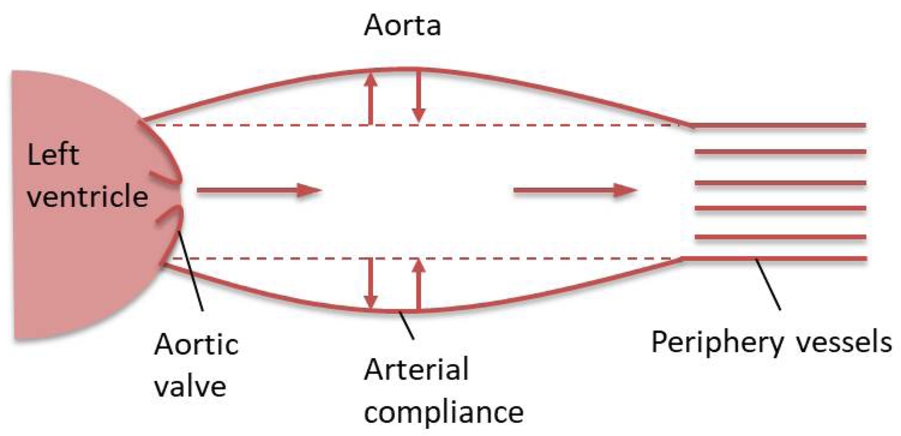
The Windkessel model takes into consideration the following parameters as shown in Fig. 1 and characterizes peripheral resistance of the aortic valve, arterial compliance and peripheral resistance of the vessels:
• Resistance of the aortic valve (r) refers to the flow resistance encountered by the blood as it is pumped from the heart to the arterial system.
• Arterial compliance (
• Peripheral resistance (
The original version of the Windkessel is the 2-element model, which consists of a capacitor (C) to account for arterial compliance (
The Windkessel model takes into account the effects of arterial compliance and total peripheral resistance determined by the systolic and diastolic phases of the cardiac cycle. As shown in Table 1,
(1)
(2)
The differential equation of the 3-element Windkessel model is given as:
(3)
In the 2- or 3-element Windkessel model, no defined time-varying potential
Given that it does not have a stable operating state, an astable multivibrator oscillates back and forth between reset and set states. Also referred to as clock circuits, astable multivibrators are used to provide a clock signal to digital circuits so that these can operate. Figure 3a shows a circuit diagram of an astable multivibrator. A characteristic of an astable multivibrator is the availability of two outputs (0 and 1) that are logically inverse. The action of the transistors in a multivibrator can be considered an ideal switch. If a transistor is off, it does not draw a current through the collector-emitter and is an open-circuit. Thus, the power supply voltage
Fig. 2
Waveforms of an astable multivibrator.
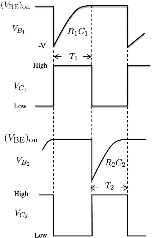
The period of the wavefoms
(4)
By using equation (4), the voltage across the capacitor
(5)
(6)
For this circuit to work,
(7)
In our design, the astable multivibrator has the component values of
(8)
(9)
(10)
According to the calculations,
Fig. 3
Proposed Windkessel model: (a) astable multivibrator circuit; (b) inverter circuit.
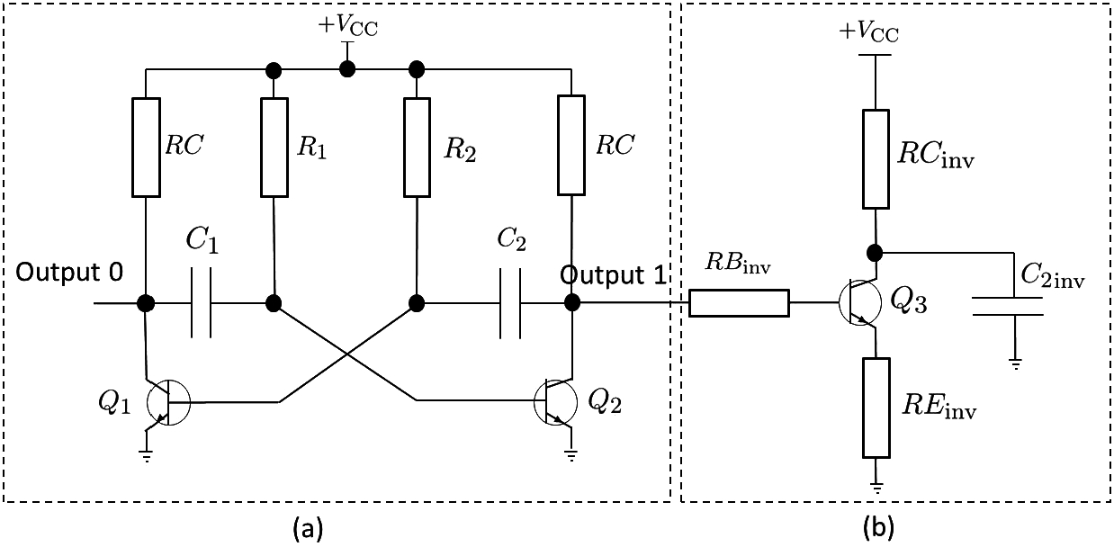
The astable multivibrator followed by an inverter (see Fig. 3b) is sufficient to obtain cardiac events during the cardiac cycle. The inverter circuit operates in the following way: If the input to the inverter is logical 0, the transistor of that circuit is held in cutoff such that there is no base current and the base-emitter appears as an open circuit. If there is no base current, there is no collector current and the output voltage is the supply voltage value. If the input to the inverter is logical 1 (12 V), the transistor becomes saturated and the transistor begins to turn on. When the output waveform of the collector of the transistor
The inverter circuit represents the aortic valve of the heart. A resistor
The astable multivibrator represents the left heart from the perspective of physiology. The transistor
In the diastole phase, the LV is relaxed. In this case, the collector voltage of transistor
Moreover, when the inverter circuit is connected to the collector of the
In the systole phase, the LV contracts and pumps the blood out of the arteries. At the same time, when the LA is relaxed, the voltage drop on the collector of
4.2Agent-Based Blood Vessel Model
Agent-based modelling and simulation (ABMS) is a rule-based computational modelling approach that focuses on rules and interactions among the individuals or components of a real system. ABMS is useful for representing, creating, analysing, and experimenting with artificial worlds populated by agents that behave autonomously and interact with other agents or collective entities (Di Marzo Serugendo et al., 2011). In ABMS, each agent has its own characteristics and behaviour, and each act as a component of the system. The behaviour of any given agent may affect other agents in a simulated environment. During the simulation, the agents’ interactions with each other and/or with their environment may reveal behaviour patterns not defined in the system (emergence phenomena). Time in the simulation environment is typically represented as a time step or tick count. In each time step, each agent performs actions, interacts with other agents, and/or interacts with other components in the environment.
In a previous study (Bora et al., 2019), we have developed an agent-based blood vessel model of the CVS. However, in the present study, we observed changes in the pressure of the arterial system through the aorta when the LV pumps blood to the aorta. Thus, we have implemented an agent-based blood vessel approach to model the behaviour of the aorta.
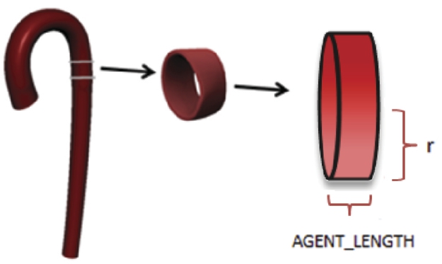
In agent-based blood vessel model, the aorta is divided into segments referred to as aorta agents (see Fig. 4), each of which mimics the aorta’s functionality.
Fig. 4
Agent-based aorta model.
Information is transferred between consecutive agents. When the LV contracts, the pressure on the first aorta agent reaches its maximum value in the cardiac cycle. This pressure value is transferred to the second aorta agent. In the next cardiac simulation cycle, the aortic pressure on the second aorta agent reaches its maximum value and is transferred to the next aorta agent, and so on. We implement the well-known pattern of publish-subscribe in order to provide interaction between the agents. Each agent subscribes itself to the corresponding agent and publishes messages in order to propagate messages to its listeners. On receiving a message, an agent updates itself (adapts itself if required) and regulates its behaviour according to the current environment situation. Each aorta agent evaluates its current situation according to its local knowledge and behaves accordingly (Bora et al., 2019).
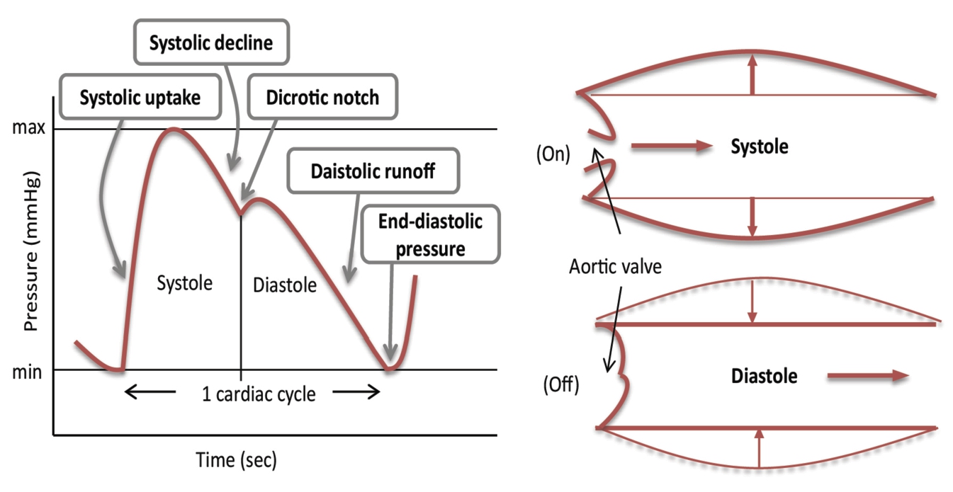
In Fig. 511, the aortic pressure waveform is represented in respect to time. The aorta can be in one of the following states in a cardiac cycle: systolic uptake, systolic decline, dicrotic notch, diastolic runoff, and end-diastolic pressure. When the LV pumps blood into the aorta, the pressure in the aorta is at its maximum value. Before the LV ejects the blood to the aorta, the pressure in the aorta is at its minimum value.
Fig. 5
Aortic pressure waveform.
We show the cardiac cycle in the state machine in Fig. 6. We use the state machine to represent the agent’s states. The state machine is an abstract concept used to design algorithms or/and describe program interactions. It is defined as an initial state, a set of input and output events, a set of new states that result from the input events, a set of possible actions that result from a new state. During a cardiac cycle, each agent is being at an agent state which is defined in the state machine at a time (Cakırlar, 2015).
Fig. 6
State machine of the aorta during a cardiac cycle.
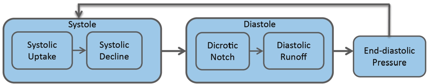
Fig. 7
Aorta agents’ behaviour.
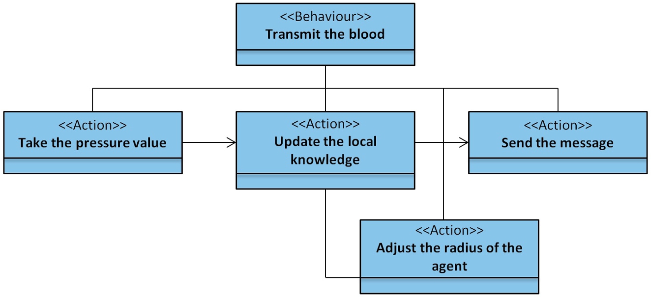
Figure 7 shows the behaviour of the aorta agents that transmit oxygen-rich blood. Aorta agents represent a specific aortic cross-section. The message transmitted through the aorta agents is that the blood pressure value is to be pumped from the LV of the heart. Each aorta agent updates the value of its pressure according to its radius and other vessel parameter values (length, resistance, volume, compliance, etc.) and sends these values to neighbour agents. If the incoming pressure value indicates that dilation is necessary, the radius of the aorta is adjusted.
At any given time, the aorta agents can be in various states: whereas some are in systolic uptake, others can be in systolic decline, dicrotic notch, diastolic runoff, or end-diastolic pressure. In order to represent a wave of pressure, a cardiac cycle is represented in 100 simulation cycles (see Fig. 5). The aorta agents’ states in a cardiac cycle that we observed and the corresponding simulation cycles (n) and formula for obtaining the value of the pressure at the nth cycle are given in Table 2.
Table 2
Aorta agent states during a cardiac cycle and associated pressure values.
| Aorta agent state | Cardiac cycle phase | Simulation cycle (n) | Pressure (n) |
| Systolic uptake | Systole | 1–20 | Pressure( |
| Systolic decline | Systole | 21–30 | Pressure( |
| Dicrotic notch | Diastole | 31–40 | Pressure( |
| Diastolic runoff | Diastole | 41–90 | Pressure( |
| End-diastolic pressure | 91–100 | Pressure( |
In Table 2, the pressure values for each state of agents are calculated uniformly.
5Results
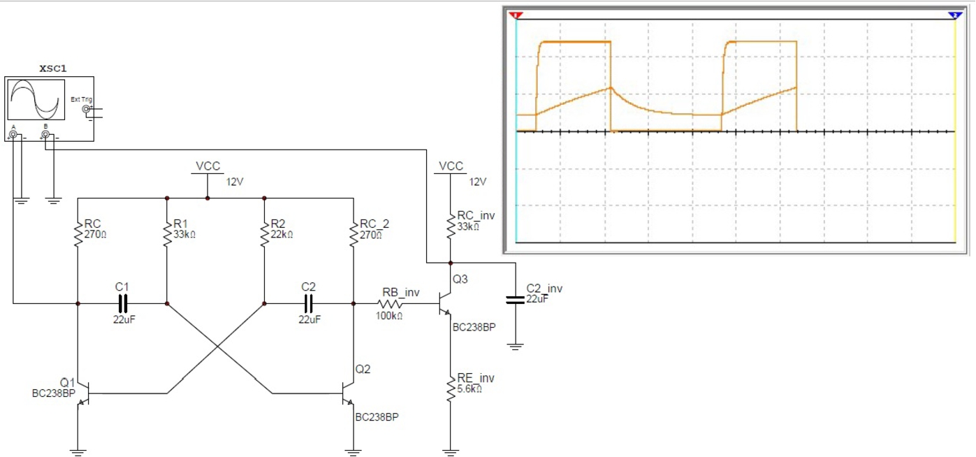
In this study, we offered two distinct methods for observing aortic behaviour in the CVS: (1) a Windkessel model and (2) an agent-based model. The results of the Windkessel model approach are observed both in experimental and simulation environments. It is very difficult to capture very small frequency signals. Therefore, the observed results were tested in a simulation environment (see Fig. 8). We could capture the image of the test results with the component values of
Fig. 8
Proposed Windkessel model in the simulation environment.
In the other simulation approach, we developed our model in Java language, using Repast Simphony tool. We run the simulation at 1000 simulation cycles (tick counts). We defined one cardiac cycle as 100 simulation cycles. In Table 3 below, we list all the global parameters used by an aorta agent in the algorithm of the model and their definitions.
Table 3
Global parameters for the aorta model of the human CVS.
| Global parameters | Definition | Initial values |
| Pressure MIN (mmHg) | Minimum pressure value for the aorta agent | U(60, 89) |
| Pressure MAX (mmHg) | Maximum pressure value for the aorta agent | U(130,139) |
| Pressure state | Pressure state of the aorta agent | None |
| Aort initial radius (cm) | Aorta initial radius value for the current simulation | 1.25 |
| Cycle duration (tick count) | Duration of the cardiac cycle | 100 |
| Agent cunt | The number of the aorta agents in the current simulation | 50 |
| Aort length (cm) | Length of the aorta for the current simulation instance | 50 |
| Tapering factor | Tapering factor value | 0.0315 |
| Viscosity (P) | Viscosity value for the current simulation | 0.0333 |
| Density (kg/m3) | Density value of the blood for the aorta agent | 1.015 |
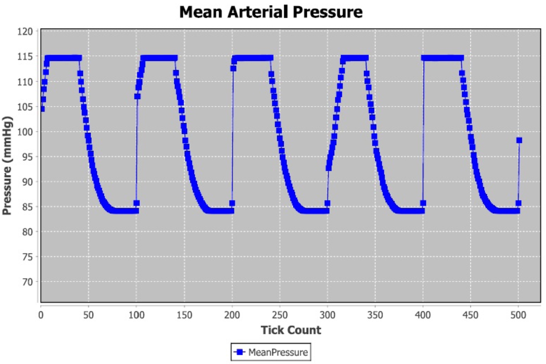
These parameters depend on the assumptions made during the design of the ABMS model. The reason for this is that agents are not modelled in cell size. Each vessel agent represents a specific vessel cross section, and therefore, first aortic radius and the aortic length values of the model are added as the simulation parameters. The general structure of the vessel is decreasing in size towards the capillaries from the first aortic entrance. However, the first aortic radius can be calculated based on a known vessel structure, age and gender. In addition, blood density and fluidity cause blood vessels to behave differently during transport of blood through the vessels. In addition, due to some internal calculations, it is necessary to define certain constants as information sources. The mean arterial pressure pumped from the LV agent to the aorta agents is shown in Fig. 9.
Fig. 9
Mean arterial pressure over time.
6Validation of the Models
Any effort to assess a simulation relies on a combination of protocols properly applied together with the application of analytical expertise as well as a framework within which initial predictions are proposed and a retrodictive consideration offered. In the present article, the behaviour of agents takes place in relation to the parameters of a healthy person in usual circumstances. Further, the study relies on field experts to determine the boundary ranges of the parameters, the default values, and the results reported.
Emprical knowledge is created in building and validating models of this nature, such that they tend to be associated with processes described as the “Empirical Validation of Agent-Based Models”. Such models are defined by characteristics that have been empirically confirmed in relation to a specific domain. Scientific methods of investigation and analysis are used to collect and describe data in both quantitative and qualitative terms (David et al., 2017). On this basis, through an empirical validation of agent-based models, there is potential to establish a significant relationship between the model and a context-specific problem domain with boundaries clearly and accurately delineated. The two models in the present article are validated in reference to the specific inputs to and outputs of each. For the agent-based model, the input parameters, which include pressure, resistance, and compliance, are understood as having an effect on the behaviour of the agents. The input validation can be assessed on the basis of a structural assumption pertaining to the behaviour and/or the interactions of the agents (Fagiolo and Richiardi, 2018). In light of the micro-level behaviours in the agent-based simulation, behaviour at the macroscopic scale is compared to behaviour identified in the target (David et al., 2017). Depending on the behavioural parameters of the cardiovascular system, it is possible to monitor the global behaviour of CVS. In the body of relevant research, the behaviour seen at the macro-level provides a basis for performing tests at the micro-level when the agent-based model is implemented (Deviha et al., 2013; Jayalalitha et al., 2007). Further, it is well-established that any given model must be operationalized and its results analysed in relation to a theoretical foundation (Frigg and Hartmann, 2020). In regard to simplification and abstraction, the mechanisms operational in these models are ordinarily described in formalised or mathematical terms (David et al., 2017). The Windkessel model, for example, includes a description of the effects of arterial compliance and total peripheral resistance as established by the systolic and diastolic activity in cardiac functioning. The resistance behaviour exhibited by each agent against the blood flow becomes apparent in line with Ohm’s law.
Whereas physiological parameters can be modelled using hemodynamic principles, agents’ behaviour can be monitored in the simulation (David et al., 2017). Therefore, it is possible to determine whether or not classes of behaviour identified in the target system are present in the simulation. For example, it can be determined whether or not the actions and behaviour of the agents, the interactions between them, and their collective behaviour accurately represent the conception and representation of the target system. These are important issues that researchers have endeavoured to resolve. For this reason, engaging researchers with a high level of expertise in the domain to both create and validate the model is vital. It falls to the expert researcher, therefore, to experimentally validate whether the hypotheses receive full, partial, or even no support by operationalizing the model and describing the results that accrue in computational terms. However, models can be readily connected and compared and contrasted with other models, extended with further mechanisms, and refined as more data pertinent to the model’s accuracy for a given purpose are collected (David et al., 2017).
7Discussion and Conclusions
Several approaches to the Windkessel models are documented in the literature; each focuses on aspects of electrical modelling of arterial system as elaborated in Section 3. However, none of them concerns the timing perspective of output of the Windkessel circuit. The astable multivibrator may be connected to the Windkessel circuits documented in the literature in order to improve timing in their models. We have established the proposed Windkessel model in the real environment as a digital electronic circuit based on the theoretical, formula-based, physics laws. Moreover, we have modelled and simulated the agent-based blood vessel in the Repast Symphony environment as rule-based according to the agents’ roles and behaviours. Considering agent-based model, the role of the blood vessels is to deliver the blood to various parts of the body. The blood density and fluidity of the vessels during the transport of blood within the vessels causes different behaviour. Before implementation of the agent-based blood vessel model, the agents must be determined and every actor defined outside of blood can be represented as an agent. That is why every actor can show its own and autonomous behaviour. In addition, due to some internal calculations, it is necessary to define certain constants as information sources.
In this study, an agent-based blood vessel model and a Windkessel model are developed in order to report a research and development study on mathematical and computational techniques used to model the behaviour of the aorta. From the results, it is observed that both models’ exhibited the same responses to their inputs which represented blood presure in the CVS. Therefore, these two models are useful for extending the studies in terms of the understanding of the dynamics of the vascular system. Besides, the Windkessel model is the first one that uses digital electronics for realizing the left heart and aorta behaviours’ in terms of timing perspective and electrical quantities. While this model still takes into consideration hemodynamic of the arterial system such as compliance and resistance, it also represents the left heart, aortic valve, and aorta during the systole and diastole phases. Moreover, an agent-based blood vessel approach to modelling the behaviour of the aorta is implemented and changes in the pressure of the arterial system through the aorta are reported in this paper.
Notes
1 Yartsev, A. (2018). Normal arterial line waveforms [Online]. Website https://derangedphysiology.com/main/cicm-primary-exam/required-reading/cardiovascular-system/Chapter%20760/normal-arterial-line-waveforms [accessed 2 October 2020].
References
1 | Al-Adwan, I., Khawaldah, M.A., Asad, S., Al Rawashdeh, A. ((2013) ). Design of an adaptive fuzzy-based control system using genetic algorithm over a pH titration process. International Journal of Research and Reviews in Applied Sciences, 17 (2): , 177–184. |
2 | Alfonso, M.R., Cymberknop, L.J., Legnani, W., Pessana, F., Armentano, R.L. (2014). Conceptual model of arterial tree based on solitons by compartments. In: Annual International Conference of the IEEE Engineering in Medicine and Biology Society, pp. 3224–3227. |
3 | Barnea, O. ((2010) ). Open-source programming of cardiovascular pressure-flow dynamics using SimPower toolbox in Matlab and Simulink. The Open Pacing, Elecrtophysiology & Therapy Journal, 3: , 55–59. |
4 | Bora, S., Evren, V., Emek, S., Çakırlar, I. ((2019) ). Agent-based modeling and simulation of blood vessels in the cardiovascular system. SIMULATION, 95(4): , 297–312. |
5 | Broemser, P., Ranke, O. ((1930) ). Über die messung des schlagvolumens des herzens auf umblutigem weg. Zeitschrift für Biologie, 90: , 467–507. |
6 | Cakırlar, I. (2015). Development of Test Driven Development Methodology For Agent-Based Simulations. PhD thesis, Ege University, Izmir, Turkey. |
7 | Capoccia, M. ((2015) ). Development and characterization of the arterial windkessel and its role during left ventricular assist device assistance. Artificial Organs, 39(8): , 138–153. |
8 | Cardelli, L. ((2005) ). Abstract machines of systems biology. In: Priami, C., Merelli, E., Gonzalez, P., Omicini, A. (Eds.), Transactions on Computational Systems Biology III, Lecture Notes in Computer Science, Vol. 3737: . pp. 145–168. |
9 | Craig, E.C. ((1994) ). Astable Multivibrator. Springer, New York. |
10 | Creigen, V., Ferracina, L., Hlod, A.V., Mourik van, S., Sjauw, K., Rottschäfer, V., Vellekoop, M., Zegeling, P.A. ((2007) ). Modeling a heart pump. In: Proceedings 58th European Study Group Mathematics with Industry (ESGI58/SWI2007), 29 January–2 February 2007, Utrecht, The Netherlands. Utrecht University, Netherlands, pp. 7–25. |
11 | David, N., Fachada, N., Rosa, A.C. ((2017) ). Verifying and validating simulations. In: Edmonds, B., Meyer, R. (Eds.), Simulating Social Complexity. Understanding Complex Systems. Springer, Cham. https://doi.org/10.1007/978-3-319-66948-9_9. |
12 | Deviha, V.S., Rengarajan, P., Hussain, R.J. ((2013) ). Modeling blood flow in the blood vessels of the cardiovascular system using fractals. Applied Mathematical Sciences, 7(11): , 527–537. |
13 | Di Marzo Serugendo, G., Gleizes, M.P., Karageorgos, A. ((2011) ). Self-organising Software From Natural to Artificial Adaptation. Springer, Verlag Berlin Heidelberg. |
14 | Emek, S. (2018). Modeling and Simulation of Global Behaviors of the Self-Adaptive Systems by Using Agent Based System. PhD thesis, Ege University, Izmir, Turkey. |
15 | Fagiolo, G., Richiardi, M. ((2018) ). Empirical validation of agent-based models. In: Delli Gatti, D., Fagiolo, G., Gallegati, M., Richiardi, M., Russo, A. (Eds.), Agent-Based Models in Economics: A Toolkit. Cambridge University Press, Cambridge, pp. 163–182. https://doi.org/10.1017/9781108227278.009. |
16 | Fazeli, N., Hahn, J. ((2012) ). Estimation of cardiac output and peripheral resistance using square-wave-approximated aortic flow signal. Frontiers in Physiology, 3: , 298. |
17 | Fischer, H.P. ((2008) ). Mathematical modeling of complex biological systems: from parts lists to understanding systems behavior. Alcohol Research & Health, 31(1), 49–59. |
18 | Frank, O. ((1899) ). Die Grundform des arteriellen Pulses. Zeitschrift für Biologie, 37: , 483–526. |
19 | Frigg, R., Hartmann, S. ((2020) ). Models in science. In: Zalta, E.N. (Ed.), The Stanford Encyclopedia of Philosophy. Metaphysics Research Lab., Stanford University, Stanford. |
20 | Fuchs, H.U. ((2010) ). The Dynamics of Heat: A Unified Approach to Thermodynamics and Heat Transfer. Springer, New York. |
21 | Gostuski, V., Pastore, I., Palacios, G.R., Diez, G.V., Moscoso-Vasquez, H.M., Risk, M. ((2016) ). Time domain estimation of arterial parameters using the Windkessel model and the Monte Carlo method. Journal of Physics: Conference Series, 705: , 012028. |
22 | Guo, Z., Tay, J.C. ((2007) ). A hybrid agent-based model of chemotaxis. In: Computational Science – ICCS 2007. Springer Berlin Heidelberg, Berlin, Heidelberg, pp. 119–127. |
23 | Guyton, A.C., Hall, J.E. ((2015) ). Textbook of Medical Physiology. Elsevier Inc., Philadelphia. |
24 | Hlavac, M., Holcik, J. (2020). Windkessel model analysis in MATLAB. http://www.ecmosimulation.com/data/Hlavac.pdf. Accessed 28 October 2020. |
25 | Jayalalitha, G., Shanthoshini Deviha, V., Uthayakumar, R. ((2007) ). Fractal model of he blood vessel in cardiovascular system. In: 15th International Conference on Advanced Computing and Communications (ADCOM 2007), pp. 175–182. |
26 | Kokalari, T., Karaja, T., Guerrisi, M. ((2013) ). Review on lumped parameter method for modeling the blood flow in systemic arteries. Journal of Biomedical Science and Engineering, 6: (1), 92–99. |
27 | Li, Y., Lawley, M.A., Siscovick, D.S., Zhang, D., Pagan, J.A. ((2016) ). Agent-based modeling of chronic diseases: a narrative review and future research directions. Preventing Chronic Disease, 13: , 69. |
28 | Ma’ayan, A. (2017). Complex systems biology. Journal of the Royal Society Interface, 14(134). |
29 | Macal, C.M., North, M.J. (2009). Agent-based modeling and simulation. In: WSC’09 Winter Simulation Conference, pp. 86–98. |
30 | Mei, C.C., Zhang, J., Jing, H.X. ((2018) ). Fluid mechanics of Windkessel effect. Medical & Biological Engineering & Computing, 56: , 1357–1366. |
31 | Motta, S., Pappalardo, F. ((2012) ). Mathematical modeling of biological systems. Briefings in Bioinformatics, 14: (4), 411–422. |
32 | North, M.J., Tatara, E., Collier, N.T., Ozik, J. (2007). Decision and information sciences. In: Visual Agent-Based Model Development with Repast Simphony, University of Chicago and PantaRei Corporation. |
33 | Northrop, R.B. ((2010) ). Introduction to Complexity and Complex Systems. CRC Press, Boca Raton. |
34 | Olufsen, M.S., Peskin, C.S., Kim, W.Y.-, Pedersen, E.M., Nadim, A., Larse, J. ((2000) ). Numerical simulation and experimental validation of blood flow in arteries with structured-tree outflow conditions. Annals of Biomedical Engineering, 28: (11), 1281–1299. |
35 | Ortiz-Leon, G., Vilchez-Monge, M., Montero-Rodriquez, J.J. (2014). Simulations of the cardiovascular system using the cardiovascular simulation toolbox. In: 5th Workshop on Medical Cyber-Physical Systems, pp. 28–37. |
36 | Quarteroni, A., Veneziani, A., Zunino, P. ((2002) ). Mathematical and numerical modeling of solute dynamics in blood flow and arterial walls. SIAM Journal on Numerical Analysis, 39: (5), 1488–1511. |
37 | Rocha, L.M. (2020). Complex Systems Modeling: Using Metaphors From Nature in Simulation and Scientific Models. https://homes.luddy.indiana.edu/rocha/publications/complex/csm.html. Accessed 2 October 2020. |
38 | Westerhof, N., Lankhaar, J.W., Westerhof, B.E. ((2008) ). The arterial Windkessel. Medical & Biological Engineering & Computing, 47: (2), 131–141. |


