
Experimental Analysis of Algebraic Modelling Languages for Mathematical Optimization
Abstract
In this work, we perform an extensive theoretical and experimental analysis of the characteristics of five of the most prominent algebraic modelling languages (AMPL, AIMMS, GAMS, JuMP, and Pyomo) and modelling systems supporting them. In our theoretical comparison, we evaluate how the reviewed modern algebraic modelling languages match the current requirements. In the experimental analysis, we use a purpose-built test model library to perform extensive benchmarks. We provide insights on which algebraic modelling languages performed the best and the features that we deem essential in the current mathematical optimization landscape. Finally, we highlight possible future research directions for this work.
1Introduction
Many real-world problems are routinely solved using modern optimization tools (e.g. Abhishek et al., 2010; Fragniere and Gondzio, 2002; Groër et al., 2011; Paulavičius and Žilinskas, 2014; Paulavičius et al., 2020a, 2020b; Pistikopoulos et al., 2015). Internally, these tools use the combination of a mathematical model with an appropriate solution algorithm (e.g. Cosma et al., 2020; Fernández et al., 2020; Gómez et al., 2019; Lee et al., 2019; Paulavičius and Žilinskas, 2014; Paulavičius et al., 2014; Paulavičius and Adjiman, 2020; Stripinis et al., 2019, 2021) to solve the problem at hand. Thus, the way mathematical models are formulated is critical to the impact of optimization in real life.
Mathematical modelling is the process of translating real-world business problems into mathematical formulations whose theoretical and numerical analysis can provide insight, answers, and guidance beneficial for the originating application (Kallrath, 2004), including the current Covid-19 pandemic (Rothberg, 2020). Algebraic modelling languages (AMLs) are declarative optimization modelling languages, which bridge the gap between model formulation and the proper solution technique (Fragniere and Gondzio, 2002). They enable the formulation of a mathematical model as a human-readable set of equations while not requiring to specify how the described model should be solved or what specific solver should be used.
Models written in an AML are known for the high degree of similarity to the mathematical formulation. This aspect distinguishes AMLs from other types of modelling languages, like object-oriented (e.g. OptimJ), solver specific (e.g. LINGO), or general-purpose (e.g. TOMLAB) modelling languages. Such an algebraic design approach allows practitioners without specific programming or modelling knowledge to be efficient in describing the problems to be solved. It is also important to note that AML is then responsible for creating a problem instance that a solution algorithm can tackle (Kallrath, 2004). Since many AMLs are integral parts of a specific modelling system, it is essential to isolate a modelling language’s responsibilities from the overall system. In general, AMLs are sophisticated software packages that provide a crucial link between an optimization model’s mathematical concept and the complex algorithmic routines that compute optimal solutions. Typically, AML software automatically reads a model and data, generates an instance, and conveys it to a solver in the required form (Fourer, 2013).
From the late 1970s, many AMLs were created (e.g., GAMS, McCarl et al., 2016, AMPL, Fourer, 2003) and are still actively developed and used today. Lately, new open-source competitors to the traditional AMLs started to emerge (e.g., Pyomo, Hart et al., 2017, 2011, JuMP, Dunning et al., 2017; Lubin and Dunning, 2015). Therefore, we feel that a review and comparison of the traditional and emerging AMLs are needed to examine how the current landscape of AMLs looks.
The remainder of the paper is organized as follows. In Section 2, we review the essential characteristics of AMLs and motivate our selection of AMLs for the current review. In Section 3, we investigate how the requirements for a modern AML are met within each of the chosen languages. In Section 4, we examine the characteristics of AMLs using an extensive benchmark. In Section 5, we investigate the presolve impact on solving. Finally, we conclude the paper in Section 6.
2Algebraic Modelling Languages
The first algebraic modelling languages, developed in the late 1970s, were game-changers. They allowed separating the model formulation from the implementation details (Kallrath, 2004) while keeping the notation close to the problem’s mathematical formulation (Fragniere and Gondzio, 2002). Since the data appears to be more volatile than the problem structure, most modelling language designers insist on the data and model structure being separated (Hürlimann, 1999). Therefore, the central idea in modern AMLs is the differentiation between abstract models and concrete problem instances (Hart et al., 2011). A specific model instance is generated from an abstract model using data. This way, the model and data together specify a particular instance of an optimization problem for which a solution can be sought. This is realized by replicating every entity of an abstract model over the different elements of the data set. Such a feature often is referred to as a set-indexing ability of the AML (Fragniere and Gondzio, 2002).
Essential characteristics of a modern AML could be defined in the following way (Kallrath, 2004):
The algebraic expressions are useful in describing individual models and describing manipulations on models and transformations of data. Thus, almost as soon as AML became available, users started finding ways to adapt model notations to implement sophisticated solution strategies and iterative schemes. These efforts stimulated the evolution within AMLs of scripting features, including statements for looping, testing, and assignment (Fourer, 2013). Therefore, scripting capabilities are an integral part of AMLs.
For this review, we have chosen five AMLs: AIMMS, AMPL, GAMS, JuMP, and Pyomo. The selection was based on the following criteria:
• AMLs which won 2012 INFORMS Impact Prize award22 dedicated to the originators of the five most important algebraic modelling languages: AIMMS, AMPL, GAMS, LINDO/LINGO, and MPL;
• the popularity of AMLs based on NEOS Server model input statistics for the year 2020;33
• open-source options that are attractive for the academic society or in situations where budgets are tight.
We have chosen to include GAMS and AMPL based on NEOS Server popularity, respectively, with 49% and 47% share of jobs executed via the NEOS platform in 2020. AIMMS was added as an example of AML with a graphical application development environment. JuMP and Pyomo were included as the most prominent open-source AMLs. We have decided to exclude MPL since it has not been updated for the last five years. We have also excluded LINGO as a solver specific modelling language.
3Comparative Analysis of AMLs Characteristics
In the following section, we investigate how each of the chosen languages meets the requirements for a modern AML defined in the previous section. The websites of the AMLs and vendor documentation are used for this comparison. Any support of the identified features and capabilities are validated against the documentation the suppliers of the AMLs provide. Besides, an in-depth survey concluded by Robert Fourer in Linear Programming Software Survey (Fourer, 2017) is also used as a reference. Later on, a more practical comparison of AML characteristics is conducted to identify the potential ease of use of AML in daily work.
3.1Comparative Analysis of the Features
We start by analysing how selected AMLs satisfy the three essential characteristics defined in the previous Section 2. In all reviewed AMLs, optimization problems are represented in a declarative way. Furthermore, since all of them are part of a specific modelling system, a clear separation between problem definition and the solution process in the context of the modelling system exists. The separation between the problem structure and its data is supported in all reviewed languages. It should be noted that GAMS, JuMP, and Pyomo also allow initiating data structures during their declaration, while AIMMS and AMPL only support it as a separate step in the model instance building process. However, while it might be convenient for building a simple model, we do not consider the lack of direct data structure initiation as an advantage since, in real-world cases, it is rarely needed. Therefore, we can conclude that all reviewed languages fulfill the essential characteristics of modern AMLs.
Table 1
Overviewof AMLs features.
| Feature | AIMMS | AMPL | GAMS | JuMP | Pyomo | |
| Modelling | Independent | Yes | Yes | Yes | Yes | Yes |
| Scripting | Yes | Limited | Limited | Yes | Yes | |
| Data | Input | Yes | Limited | Limited | Yes | Yes |
| Manipulation | Yes | No | No | Yes | Yes | |
| Solvers | Total | 13 | 47 | 35 | 14 | 25 |
| Global | 1 | 4 | 9 | 2 | 1 | |
| LP | 8 | 17 | 21 | 9 | 10 | |
| MCP | 2 | 1 | 5 | 1 | 1 | |
| MINLP | 3 | 6 | 15 | 3 | 6 | |
| MIP | 5 | 14 | 16 | 6 | 8 | |
| MIQCP | 5 | 5 | 20 | 3 | 4 | |
| NLP | 6 | 19 | 17 | 7 | 10 | |
| QCP | 6 | 9 | 21 | 6 | 6 | |
| Presolving | Yes | Yes | No | No | No | |
| Visualization | Yes | No | No | No | No | |
| License | General | Paid | Paid | Paid | Free | Free |
| Academic | Paid | Free | Free | Free | Free |
Next, in Table 1, we provide an overview of the key features each AML supports. For creating such a summary, we used the information provided by the AML vendors on their websites. All reviewed AMLs allow modelling problems in a solver independent manner. Additionally, AIMMS, JuMP, and Pyomo provide a more powerful way to define advanced algorithms using R, Julia, or Python programming languages. The ease of data input for the model differs among AMLs. While all of them support input from a flat file, some more advanced scenarios such as reading data from relational databases are more straightforward in AIMMS, JuMP, or Pyomo. AMPL and GAMS require a complicated setup instead (e.g. using ODBC drivers) to access the database. Wherein JuMP or Pyomo, a standard Julia or Python driver could be used to get data from relational and any other type of database supported by Python or Julia. Manipulation (e.g. transformation) of data is only supported by AIMMS, JuMP, and Pyomo.
When it comes to solver support, AMPL is the one supporting the most. However, it should be noticed that the categorization of solvers by supported problem types is different among vendors. Thus, in this comparison, we have reflected the information available from vendors harmonizing it across all of them. Solvers supported by JuMP and Pyomo require additional explanation. First, both AMLs support solvers compatible with AMPL (via AmplNLWriter package or ASL interface). Therefore, any solver that is equipped with an AMPL interface can be used by JuMP or Pyomo. This could allow us to state that JuMP and Pyomo support all AMPL solvers. However, we have excluded solvers supported via the AMPL interface. It might be needed for some commercial solvers to request a particular version from the solver’s vendor that comes with the AMPL interface. Second, since both AMLs are open-source, multiple third-party packages add support for specific solvers for each of AMLs. In Section 1, we counted only the solvers mentioned on the official JuMP and Pyomo websites.
Presolving capabilities are only available in AIMMS and AMPL. JuMP and Pyomo have programming interfaces for creating custom presolvers, however, none of them are provided out of the box. Only AIMMS provides a visualization of the solver results out of the box. Using Python or Julia libraries, it is possible to visualize the results produced by Pyomo and JuMP. However, it requires custom development, and none of the standard JuMP or Pyomo libraries are supporting that.
It is important to conclude that JuMP and Pyomo are open-source AMLs built on top of general-purpose programming languages, making them fundamentally different from the competitors. This allows researchers familiar with Julia or Python to learn, improve, and use JuMP or Pyomo much more comfortably. At the same time, it is practically impossible to introduce improvements to commercial counterparts.
3.2Practical Comparison of AMLs
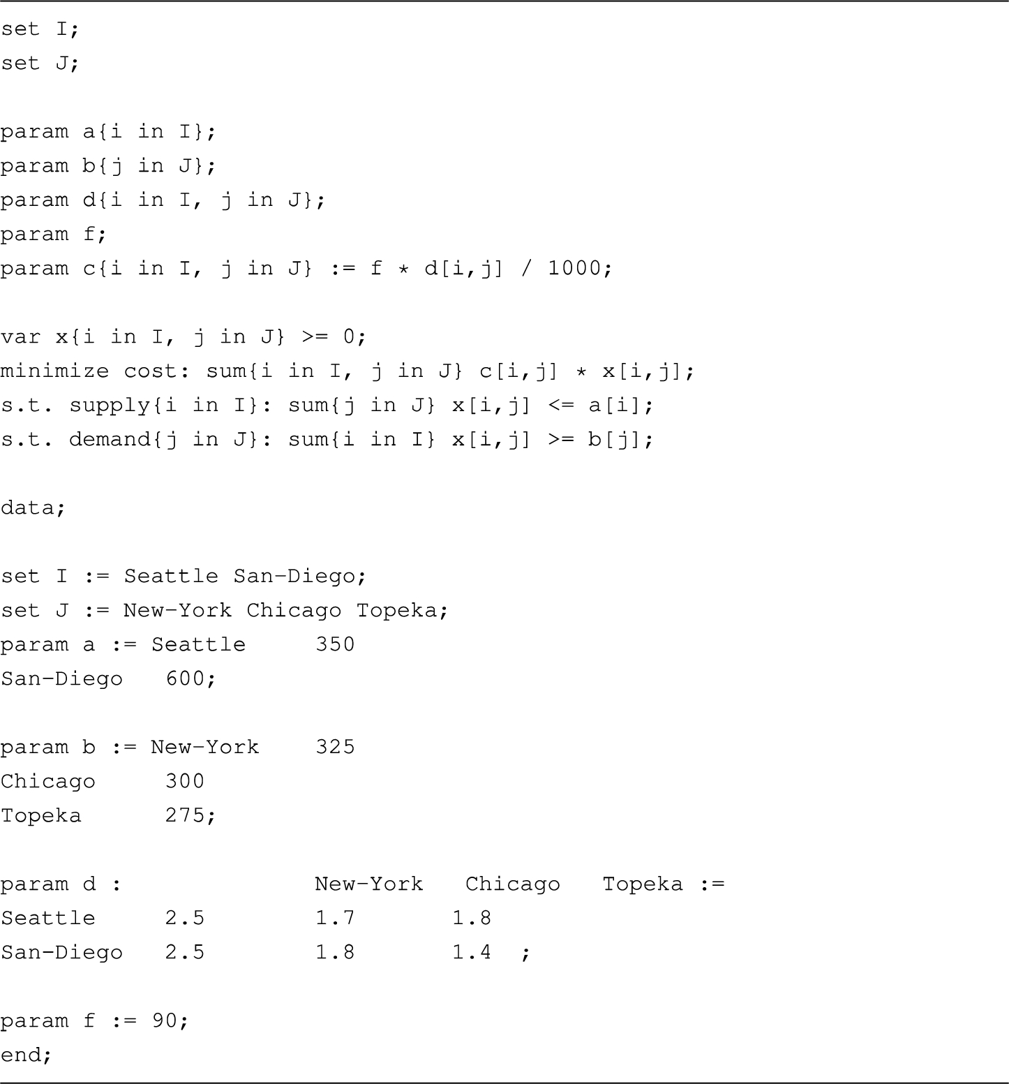
For the first practical comparison of the selected AMLs, a classical Dantzig Transportation Problem was chosen (Dantzig, 1963). In this problem, we are given the factories’ supplies and the markets’ demands for a single commodity. We have also given the unit costs of shipping the product from factories to the markets. The goal is to find the least costly shipping schedule that meets the requirements at markets and supplies at factories.
The transportation problem formulated as a model in all five considered AML is compared based on the following criteria:
• model size in bytes;
• model size in the number of code lines;
• model size in the number of language primitives used;
• model instance creation time.
Since the transportation problem is a linear programming (LP) type of problem, we have chosen to measure the model instance creation time as the time needed to export a concrete model instance to MPS44 format supported by most LP solvers. The following sources provided sample implementations of the transportation problem for the AMLs under consideration:
Table 2
Comparison of transportation problem models.
| Criteria | AIMMS | AMPL | GAMS | JuMP | Pyomo |
| Size in bytes | 2229 | 683 | 652 | 632 | 1235 |
| Lines of code | 68 | 24 | 31 | 18 | 29 |
| Primitives used | 9 | 5 | 8 | 4 | 6 |
A comparison of the sample Transportation Problem model’s characteristics in all reviewed AMLs is given in Table 2. The simplification of the model implementations provided in the literature sources is made in the following way:
• all optional comments, explanatory texts, and documentation are removed;
• all empty lines are excluded;
• parts of the code responsible for calling the solver and displaying results are omitted;
• while counting AML primitives generic functions (sum, for), data loading directives (data), arithmetical and logical operators are excluded.
It can be seen from Table 2 that models implemented in AMPL, GAMS, and JuMP are the most compact ones, while the model written in AIMMS is much more verbose, and Pyomo lies in the middle. AIMMS propagates the creation of models using a graphical user interface (GUI) while keeping the model’s source code hidden from the modeller. Naturally, there is not much focus on how the model is stored. We can argue that while the GUI-based approach might be convenient to some modellers, it enforces greater vendor lock-in and makes the model’s extensibility and maintainability harder.
While comparing the number of language primitives required to create a model, JuMP and AMPL showed the best results, which allows us to predict that these modelling languages might have a more gentle learning curve. Therefore, we can conclude that in the context of the reviewed algebraic modelling languages, JuMP allows formulating an optimization problem most concisely.
The creation time of the transportation problem model instance defined in each AMLs was used to measure a model loading. The process was done in the following steps:
1. loading model instance from a problem definition written in the native AML;
2. exporting model instance to MPS format;
3. measuring total execution time;
4. investigating characteristics of an instance model.
Table 3
Characteristics of the created transportation model instances.
| Characteristic | AMPL | GAMS | JuMP | Pyomo |
| Constraints | 6 | 6 | 6 | 6 |
| Non zero elements | 13 | 19 | 13 | 13 |
| Variables | 7 | 7 | 7 | 7 |
The characteristics of the created model instances can be seen in Table 3. We can conclude that all modelling languages have created a model instance using the same amount of variables and constraints. However, the definition of nonzero elements is different between GAMS and other modelling systems.
Table 4
Total time of consecutive transportation model instance creation runs.
| No. of runs | AMPL | GAMS | JuMP | Pyomo |
| 1 run | 30 ms | 170 ms | 28341 ms | 720 ms |
| 10 runs | 220 ms | 1730 ms | 32199 ms | 7280 ms |
| 100 runs | 2130 ms | 16490 ms | 58151 ms | 79600 ms |
In Table 4, the benchmark results of model instance creation time are provided. We have tried to run multiple consecutive model instance creations (10 runs, 100 runs) to identify if the modelling system uses any caching. We can exhibit that AMPL showed significantly better results compared to others. This allows concluding that AMPL is the most optimized from a performance point of view. On the other hand, the poor JuMP performance confirms the Dunning et al. (2017) statement that JuMP has a noticeable start-up cost1010 of a few seconds even for the smallest instances. In our case, only the initialization of the JuMP package took around 7 seconds. We also observed a significant speed-up in multiple consecutive model instances creation, which also confirms (Dunning et al., 2017) results. When a family of models is solved multiple times within a single session, this compilation cost is only paid for the first time that an instance is solved.
4Performance Benchmark of AMLs
All examined AMLs support all types of traditional optimization problems; however, it is unclear how efficiently each AML can handle large model loading and what optimizations are applied during model instance creation. It would also be of great value to analyse how each of the modelling languages performs within an area of the specific type of optimization problems (e.g. linear, quadratic, nonlinear, mixed-integer). To give such a comparison and thoroughly examine characteristics of AMLs, a more extensive benchmark involving much larger optimization problem models is needed. Therefore, a large and extensive library of sample optimization problems for the analysed AMLs has to be used.
4.1AMLs Testing Library
We have chosen the GAMS Model Library1111 as a reference for creating such a sample optimization problem suite against which future research will be done. Automated shell script gamslib-convert.sh was created to build such a library. It can be found in the tools directory of our GitHub repository (Jusevičius and Paulavičius, 2019). A detailed explanation of how the test library creation tool works and the issues identified in the GAMS Library are provided in Appendix A. As a result of the transformation, we compiled a library consisting of 296 sample problems in AMPL, GAMS, JuMP, and Pyomo scalar model formats.
4.2Model Instance Creation Time
The generated library was used to determine the amount of time each modelling system requires to create a model instance of a particular problem. We wrote load-benchmark.sh shell script available in the tools directory of our GitHub repository (Jusevičius and Paulavičius, 2019), which loads each model into the particular modelling system and then exports it to the format understandable by the solvers. We have chosen the .nl (Gay, 2005) format as the target format acceptable by the solvers, as .nl supports a wide range of optimization problem types. The benchmark measures the time the modelling system takes to perform both model instance creation and export operations.
We have chosen to exclude sample problems with conversion errors from the benchmark (more information about them in Appendix A). Only the models that were successfully processed by all modelling systems were compared. This reduced the scope of our benchmark to 268 models.
Fig. 1
Average model instance creation time.
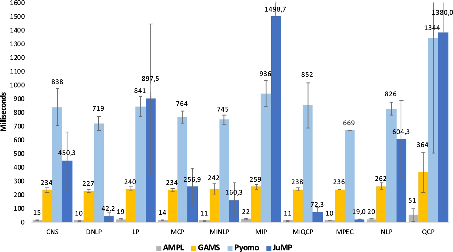
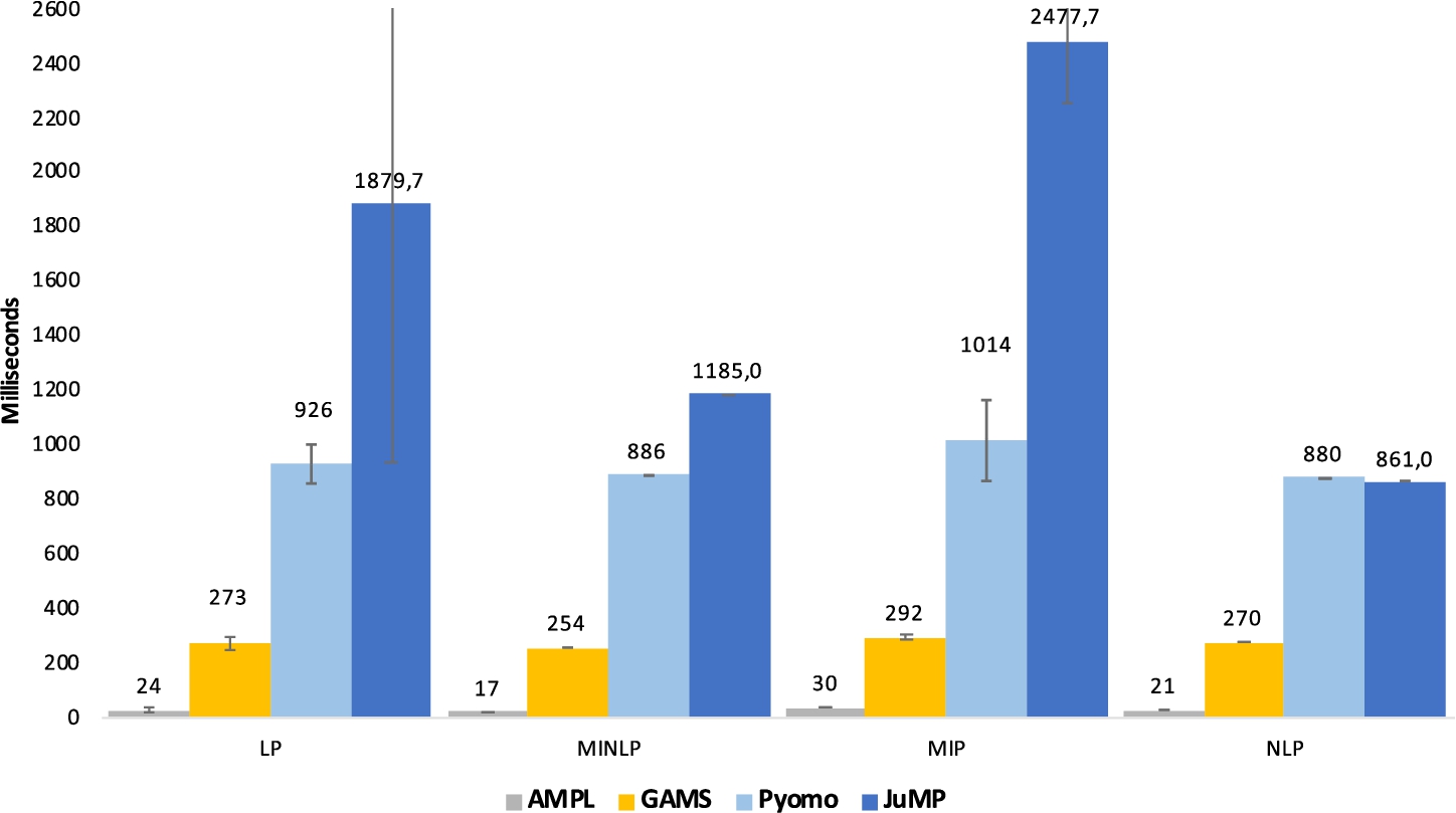
Fig. 2
Average large model instance creation time
Benchmark methodology, hardware, and software specifications can be found in our GitHub repository (Jusevičius and Paulavičius, 2019). Detailed results are available in the model-loading-times.xlsx workbook in the benchmark section of our GitHub repository (Jusevičius and Paulavičius, 2019). We have provided a summary of the average model instance creation time split by the problem type in Fig. 1. We can see the trend exhibited in the transportation problem model benchmark persists. AMPL is still a definite top performer, while JuMP and Pyomo perform the worst. There are no significant variations between different optimization problem types except for JuMP, where the model instance creation time tends to vary significantly while working with different types of problems. Moreover, as confidence intervals show, the variation between different models of the same type is also more significant once using JuMP We tend to believe this is caused by Julia’s dynamic nature and the mix of run time compilation and caching of similar JuMP models.
We have observed that the average difference between AMPL and other contenders increases when the models become larger. Comparing instance creation times of large models (models having more than 500 equations, 8 such models in the testing library) reveals 11 times the difference between AMPL and GAMS, 38 times the difference between AMPL and Pyomo, and close to 100 times the difference between AMPL and JuMP. The difference between GAMS and Pyomo stayed roughly the same – around 3.5 times. The summary of the large model instance creation time can be seen in Fig. 2.
Thus, we can conclude that out of the reviewed AMLs, AMPL is a clear top-performing AML when it comes to the model instance creation time.
4.3JuMP Benchmark
A similar time benchmark of the model instance creation has already been conducted (Dunning et al., 2017), where a smaller set of large models is used. While some of the trends exhibited in our benchmark persist (AMPL is the fastest, GAMS comes second), JuMP performance in our and Dunning et al. (2017) benchmarks differs significantly. This leads us to compare the benchmark methodology and results by conducting the benchmark described by Dunning et al. (2017).
First of all, our and their time benchmark methodologies differ. In comparison, we are trying to be solver independent and instruct AML to export the generated model instance to NL file, Dunning et al. (2017) attempt to solve the model using Gurobi solver and measure the time until Gurobi reports model characteristics. We believe that while our approach can be impacted by the system’s input/output performance, using a specific solver heavily depends on how the solver interface is implemented for a particular AML.
In the following, we have conducted two benchmarks – one as described in the original article and the second one using our method of exporting to a NL file. Results of the benchmarks can be seen in Tables 5, 6.
Table 5
JuMP benchmark using Dunning et al. (2017) method (in milliseconds).
| Model | AMPL | GAMS | Pyomo | JuMP (DIRECT) | JuMP (CACHE) |
| lqcp-500 | 2093 | 2271 | 17000 | 17388 | 37317 |
| lqcp-1000 | 8075 | 11995 | 139201 | 24590 | 44575 |
| lqcp-1500 | 18222 | 38813 | 322604 | 39370 | 66566 |
| lqcp-2000 | 32615 | 93586 | 575406 | 57597 | 88833 |
| fac-25 | 407 | 480 | 7442 | 17517 | 39245 |
| fac-50 | 2732 | 2884 | 43106 | 21331 | 47735 |
| fac-75 | 9052 | 12422 | 150550 | 31582 | 57432 |
| fac-100 | 20998 | 29144 | 393200 | 61326 | 93129 |
Before running the benchmarks, we had to rewrite some parts of the sample lqcp and facility JuMP models since syntax changes were introduced between JuMP v0.12 (used by Dunning et al. (2017)) and JuMP v0.21.5 (used by us, the latest version at the time of writing). Our benchmark was also conducted using newer versions of other AMLs–AMPL Version 20190207, GAMS v.32, Pyomo 5.7 (Python 3.8.3), Gurobi 9.0.
Additionally, we wanted to test JuMP’s new abstraction layer’s performance for working with solvers called MathOptInterface.jl (MOI). Therefore, we have tried both CachingOptimizer and DIRECT modes. As seen in Table 5, the DIRECT mode performed much better than the CachingOptimizer mode for both lqcp and facility models. An average difference in the instance creation time is close to two times, which leads us to suggest modellers evaluate MOI type choice based on specific use cases carefully.
Table 6
JuMP benchmark using export to NL method (in milliseconds).
| Model | AMPL | GAMS | Pyomo | JuMP |
| lqcp-500 | 2716 | 3265 | 39988 | 20424 |
| lqcp-1000 | 10503 | 14394 | 161404 | 80578 |
| lqcp-1500 | 25402 | 49822 | 307121 | 483268 |
| lqcp-2000 | 42780 | 125564 | >10 min | >10 min |
| fac-25 | 409 | 502 | 9420 | 8163 |
| fac-50 | 2837 | 2993 | 43087 | 31799 |
| fac-75 | 10879 | 13457 | 143286 | 219548 |
| fac-100 | 23474 | 32128 | 328170 | >10 min |
Overall, both benchmarks confirmed our observation that JuMP suffers from the long warm-up time required to pre-compile JuMP libraries. Results were also consistent with the patterns exhibited during the full gamslib benchmark performed earlier. We could not reproduce the JuMP performance metrics reported by Dunning et al. (2017), where JuMP always outperforms Pyomo. Using the original benchmark method, JuMP outperformed Pyomo only once the model size increased. However, while using our export to NL file method, JuMP, on the contrary, started to fall behind Pyomo once model size increased.
The reported differences between our and the original benchmark (Dunning et al., 2017) might be caused by multiple factors such as different JuMP versions used, improved Pyomo performance, or different Gurobi versions. It is important to stress that JuMP is a very actively developed AML that underwent significant changes during the last years. We think that it could be valuable to explore why the performance could have degraded and the reasons for such slow I/O operations performance revealed during writing to a NL file benchmark.
5Presolving Benchmark
Another performance-related feature of AMLs is the ability to presolve a problem before providing it to the solver. The presolver can preprocess problems and simplify, i.e. reduce the problem size or determine the unfeasible problem. Only two of the reviewed algebraic modelling languages provide presolving capabilities – AMPL (Fourer, 2003) and AIMMS.1212 Since we did not have the opportunity to evaluate the AIMMS modelling language practically, we could only examine AMPL presolving capabilities.
5.1Presolving in AMPL
To assess AMPL’s presolving performance, we gathered presolving characteristics while performing the model instance creation time benchmark. We have used 286 models that were successfully converted from GAMS original model to the AMPL scalar model.
Table 7
AMPL model presolving.
| Type | # models | # infeasible | Presolved (%) | Constraints reduced (%) | Variables reduced (%) |
| CNS | 4 | 0 | 100.00% | 14.63% | 31.39% |
| DNLP | 5 | 0 | 20.00% | 0.00% | 7.41% |
| LP | 57 | 0 | 36.84% | 17.81% | 9.66% |
| MCP | 19 | 0 | 89.47% | 47.00% | 8.56% |
| MINLP | 21 | 1 | 61.90% | 16.32% | 9.30% |
| MIP | 61 | 0 | 60.66% | 19.06% | 11.50% |
| MIQCP | 5 | 2 | 60.00% | 0.00% | 2.38% |
| MPEC | 1 | 0 | 100.00% | 50.00% | 0.00% |
| NLP | 101 | 2 | 47.52% | 9.71% | 11.55% |
| QCP | 10 | 0 | 60.00% | 7.10% | 2.55% |
| RMIQCP | 2 | 0 | 0.00% | 0.00% | 0.00% |
| Total | 286 | 5 | 52.80% | 18.42% | 10.73% |
A detailed report of the presolving applied to the specific model can be seen in the benchmark section of our GitHub repository (Jusevičius and Paulavičius, 2019), while the summary of it can be found in Table 7. We observed that AMPL presolver managed to simplify the models in 52.8% of the cases, out of which 5 times it could determine that the problem solution is not feasible, thus not even requiring to call the solver. On average, once applied, the AMPL presolver managed to reduce the model size by removing 18.42% of constraints and 10.73% of variables.
We can conclude that AMPL presolver is an efficient way to simplify larger problems, leading to improved solution finding performance once invoking a solver with an already reduced problem model instance. Moreover, determining not feasible models can help modellers debug the problem definition process and find errors in the model definition. This allows us to argue that presolving is an important capability of any modern AML.
5.2Presolve Impact on Solving
To evaluate if AMPL presolving has a positive impact on problem-solving, an additional benchmark was conducted. The benchmark included 146 out of 151 models to which AMPL has applied presolve in the model instance creation benchmark. Five models that AMPL presolve determined to be not feasible were excluded from the benchmark. Shell script solve-benchmark.sh provided in the tools directory of our GitHub repository (Jusevičius and Paulavičius, 2019) was created for executing such a benchmark. The script solves each model using one of the solvers and gathers output statistics to a report file.
We have chosen to solve the models using Gurobi and BARON solvers. Gurobi Optimizer (v.8.1.0) was chosen for solving LP, MIP, QCP, and MIQCP type of problems. At the same time, BARON (v.18.11.12) global solver was chosen for solving NLP, MINLP, MCP, MPEC, CNS, and DNLP problems. The solvers’ choice was motivated by the support for particular problem types.1313 and the popularity of solvers based on NEOS Server statistics.1414 Two attempts to solve each model were made. One with AMPL presolver turned on (default setting), and the second one with AMPL presolver turned off. After each run, solvers statistics, including iterations count, solve time (pure solve phase execution time), and objective, were gathered.
It is important to note that both BARON and Gurobi solvers have their presolve mechanisms (Puranik and Sahinidis, 2017; Achterberg et al., 2019). Thus the provided model is simplified by the solver too. This might result in very similar models being solved by the solver despite the AMPL presolve being turned on or off. However, the focus was on estimating AMPL presolve impact in real-life situations; therefore, a full benchmark was executed without changing the default solver behaviour. Later on, an additional benchmark was made to estimate the impact of AMPL presolve once solver presolve functionality is turned off.
Detailed AMPL presolve impact on solving report can be found in our GitHub repository’s (Jusevičius and Paulavičius, 2019) file ampl-solving-times.xlsx sheet Benchmark 1. Table 8 summarizes the positive and negative impact AMPL presolve had on solving the problems iteration and time-wise. Positive impact means fewer iterations or time was needed to solve a problem once the presolve was turned on. A negative impact means the opposite that more iterations or time was required. The impact is considered neutral if the number of iterations did not change or the required time was within the one-second tolerance level.
Table 8
Summary of AMPL presolve impact on solving.
| Iteration-wise | Time-wise | Iteration-wise (%) | Time-wise (%) | |
| Positive | 37 | 67 | 26.43% | 47.86% |
| Neutral | 74 | 40 | 52.86% | 28.57% |
| Negative | 29 | 33 | 20.71% | 23.57% |
During this benchmark, 6 models failed to be solved due to solver limitations. Two models were deemed to be not feasible, and two were solved during the AMPL presolve phase. Solvers were capable of solving 41 models during the solver’s presolve phase. Moreover, for six models, the mismatching objective was found with AMPL presolve turned on and off. Overall, AMPL presolve positively impacted 26.43% of the cases iteration-wise and 47.86% time-wise. However, it hurt 20.71% of cases iteration-wise and 23.57% time-wise.
As mentioned earlier, both BARON and Gurobi solvers have their presolve mechanisms. An additional benchmark was made to test the impact of AMPL presolve with disabled solvers presolving. Since only Gurobi allows the user to disable presolve functionality, a subset of models previously solved with Gurobi was chosen. Detailed benchmark results can be seen in our GitHub repository’s (Jusevičius and Paulavičius, 2019) file ampl-solving-times.xlsx sheet Benchmark 2. The summary of the benchmark is provided in Tables 9, 10. Gurobi could not solve two MIP problems (clad and mws) in a reasonable time once Gurobi’s presolve functionality was turned off. Those models were excluded from the benchmark.
Table 9
AMPL presolve impact with Gurobi presolve on.
| Iteration-wise | Time-wise | Iteration-wise (%) | Time-wise (%) | |
| Positive | 18 | 39 | 28.57% | 61.90% |
| Neutral | 34 | 0 | 53.97% | 0.00% |
| Negative | 11 | 24 | 17.46% | 38.10% |
Table 10
AMPL presolve impact with Gurobi presolve off.
| Iteration-wise | Time-wise | Iteration-wise (%) | Time-wise (%) | |
| Positive | 33 | 44 | 54.10% | 72.13% |
| Neutral | 10 | 0 | 16.39% | 0.00% |
| Negative | 18 | 17 | 29.51% | 27.87% |
As seen once comparing these results in Tables 9 and 10, the AMPL presolve had a greater positive effect both iteration-wise (+25.5%) and time-wise (+10.2%) once Gurobi presolve was turned off. AMPL presolve also had a less neutral impact once the solver presolving was off, thus leading to the conclusion that during the first benchmark, some models were simplified to very similar ones before actually solving them.
As we can see from the benchmarks, presolving done by AML has inconclusive effects on the actual problem solving both iterations and time-wise. However, a positive impact is always more significant than the negative one, and it especially becomes evident once the solver does not have or use its problem presolving mechanisms. This allows us to conclude that the presolving capability of AML is an important feature of a modern algebraic modelling language. We can also advise choosing AML having presolving capabilities in cases the solver used to solve the problem does not have its presolving mechanism.
6Conclusions and Future Work
From the research, we can conclude that AMPL allows us to formulate an optimization problem in the shortest and potentially easiest way while also providing the best performance in model instance loading times. It also leverages the power of model presolving, which helps the modellers in both problem definition and efficient solution finding processes. GAMS is a powerful runner-up providing very similar to AMPL problem formulation capabilities although running behind in the model instance creation time. AIMMS can be considered as being in the class of its own as it has taken a purely graphical user interface based approach. Since we could not examine the performance characteristics of AIMMS due to a lack of academic license, the performance aspect remains unclear. Open-source alternatives JuMP and Pyomo are on par with commercial competitors in the problem definition process. However, the performance of model instance creation is a bit behind compared to its competitors. JuMP suffers from noticeable environment start-up costs, while Pyomo performance tends to downgrade once the model’s size increases.
We plan to continue our research in this area by including performance comparison on automatic differentiation, adding even more large problems to our test library, and exploring the potential of parallel model instance creation support by AMLs.
Notes
1 Specifying the problem’s properties: space, set of constraints and optimality requirements.
3 NEOS Server. Solver Access Statistics: https://neos-server.org/neos/report.html.
10 Start-up cost consists of the precompilation and caching time required to prepare JuMP environment.
12 https://aimms.com/english/developers/resources/webinars/webinars-demand/algorithms/aimms-presolver/.
13 Gurobi Optimizer Reference Manual: http://www.gurobi.com; BARON User Manual: http://www.minlp.com/downloads/docs/baron%20manual.pdf.
Data Access Statement
Data underlying this article can be accessed on Zenodo at https://zenodo.org/record/4106728, and used under the Creative Commons Attribution license.
Appendices
A
ACreation of AMLs Testing Library
The automated shell script gamslib-convert.sh is available in the tools directory of our GitHub repository (Jusevičius and Paulavičius, 2019) was created to generate the AMLs testing library. The script uses GAMS Convert tool v.321515 to convert the GAMS proprietary format model to a scalar model in AMPL, GAMS, JuMP, and Pyomo formats. Characteristics of the sample problem models (number of equations, variables, discrete variables, non-zero elements, and non-zero nonlinear elements) are automatically extracted and noted. Sample problems are also grouped based on optimization problem types.
The script has two execution modes – one for converting a single model and another for converting all GAMS Library models. An example of the transportation problem from GAMS Model Library1616 converted to GAMS scalar format is shown in Listing 1.
Listing 1
Transportation problem converted to GAMS scalar model.

Listing 2
Example of a GAMS Convert error.
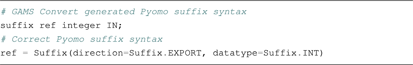
At the time of writing, there were 423 models in the GAMS Model Library. Out of them, we eliminated 66 models using GAMS proprietary modeling techniques (e.g. MPSGE, BCH Facility), 20 using general-purpose programming language features (e.g. cycles), four models tightly coupled to CPLEX and DECIS solvers. It is important to note that 35 models failed to be loaded by a fully licensed GAMS Convert tool due to execution or compilation errors. This meaning, some models in the GAMS Library are not compatible with the GAMS modelling system itself. While performing the model instance creation benchmark, we have identified that 12 AMPL, 11 JuMP, and 29 Pyomo models generated by the GAMS Convert tool had errors in them. Most of the Pyomo errors were caused by an incorrect GAMS Convert tool behaviour where the definition of the Suffix primitive uses AMPL but not Pyomo semantics. Similar issues were observed in some of the JuMP models. An example of what GAMS Convert generates and the correct Pyomo syntax can be seen in Listing 2.
B
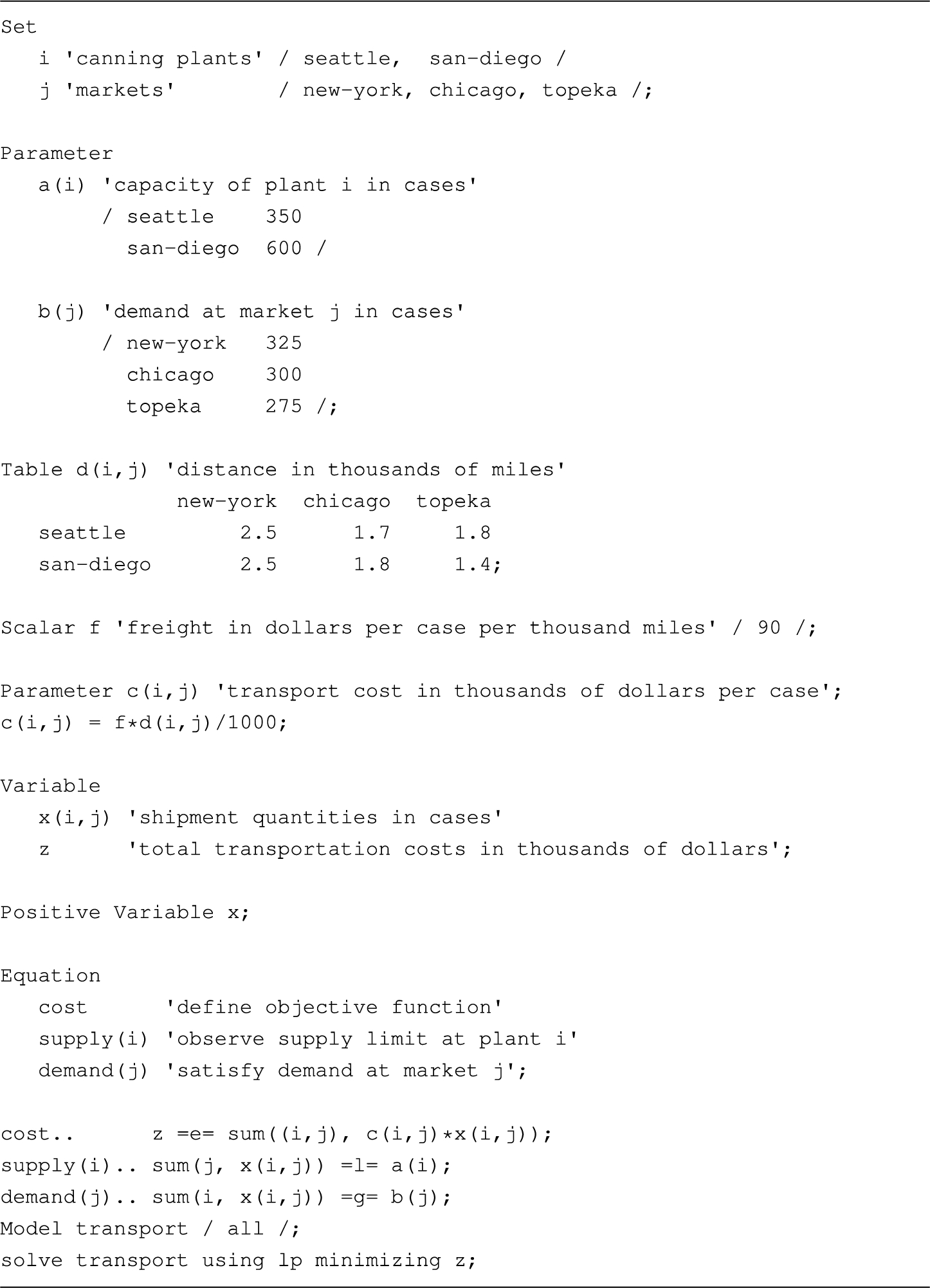
BTransportation Problem Models
Listing 3
Transportation problem defined in AMPL format.
Listing 4
Transportation problem defined in GAMS format.
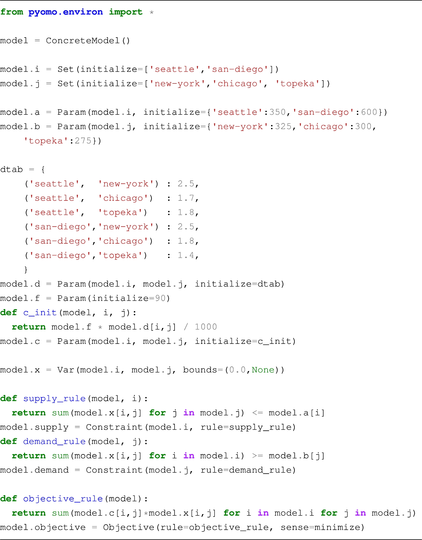
Listing 5
Transportation problem defined in Pyomo format.
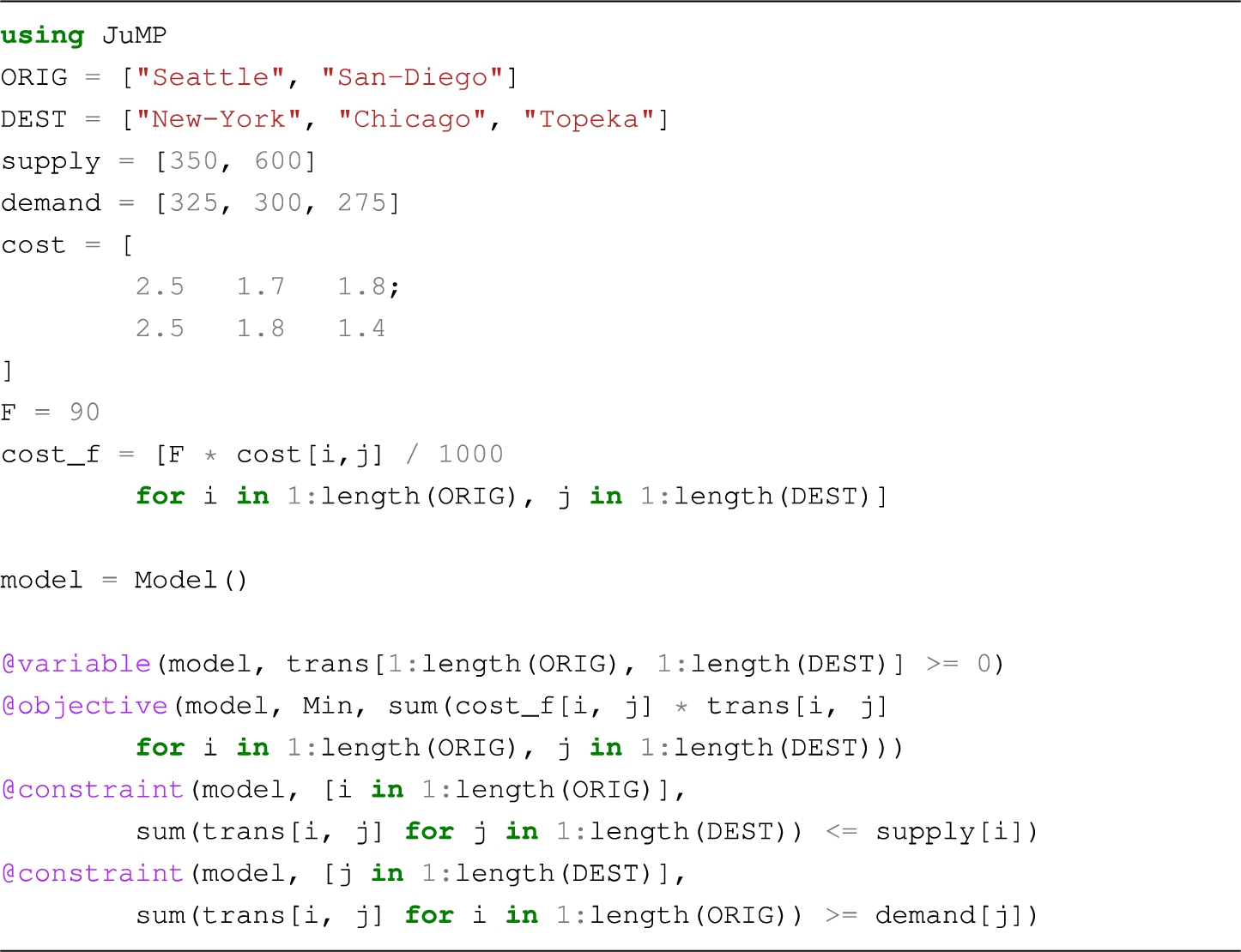
Listing 6
Transportation problem defined in JuMP format.
References
1 | Abhishek, K., Leyffer, S., Linderoth, J. ((2010) ). FilMINT: an outer approximation-based solver for convex mixed-integer nonlinear programs. INFORMS Journal on Computing, 22: (4), 555–567. https://doi.org/10.1287/ijoc.1090.0373. |
2 | Achterberg, T., Bixby, R.E., Gu, Z., Rothberg, E., Weninger, D. (2019). Presolve reductions in mixed integer programming. INFORMS Journal on Computing. https://doi.org/10.1287/ijoc.2018.0857. |
3 | Cosma, O., Pop, P.C., Dănciulescu, D. ((2020) ). A parallel algorithm for solving a two-stage fixed-charge transportation problem. Informatica, 31: (4), 681–706. https://doi.org/10.15388/20-INFOR432. |
4 | Dantzig, G.B. ((1963) ). The classical transportation problem. In: Linear Programming and Extensions. Princeton University Press, Princeton, NJ, pp. 299–315. https://doi.org/10.1515/9781400884179-015. |
5 | Dunning, I., Huchette, J., Lubin, M. ((2017) ). JuMP: a modeling language for mathematical optimization. SIAM Review, 59: (2), 295–320. https://doi.org/10.1137/15m1020575. |
6 | Fernández, P., Lančinskas, A., Pelegrín, B., Žilinskas, J. ((2020) ). A discrete competitive facility location model with minimal market share constraints and equity-based ties breaking rule. Informatica, 31: (2), 205–224. https://doi.org/10.15388/20-INFOR410. |
7 | Fourer, R. ((2003) ). AMPL: A Modeling Language for Mathematical Programming. Thomson/Brooks/Cole, Pacific Grove, CA. |
8 | Fourer, R. ((2013) ). Algebraic modeling languages for optimization. In: Encyclopedia of Operations Research and Management Science. Springer, US, pp. 43–51. https://doi.org/10.1007/978-1-4419-1153-7. |
9 | Fourer, R. (2017). Linear programming: software survey. OR/MS Today, 44(3). |
10 | Fragniere, E., Gondzio, J. ((2002) ). Optimization modeling languages. In: Handbook of Applied Optimization, pp. 993–1007. |
11 | Gay, D.M. (2005). Writing .nl files. Optimization and Uncertainty Estimation. |
12 | Groër, C., Golden, B., Wasil, E. ((2011) ). A parallel algorithm for the vehicle routing problem. INFORMS Journal on Computing, 23: (2), 315–330. https://doi.org/10.1287/ijoc.1100.0402. |
13 | Gómez, F.J.O., López, G.O., Filatovas, E., Kurasova, O., Garzón, G.E.M. ((2019) ). Hyperspectral image classification using isomap with SMACOF. Informatica, 30: (2), 349–365. https://doi.org/10.15388/Informatica.2019.209. |
14 | Hart, W.E., Watson, J.-P., Woodruff, D.L. ((2011) ). Pyomo: modeling and solving mathematical programs in Python. Mathematical Programming Computation, 3: (3), 219–260. |
15 | Hart, W.E., Laird, C.D., Watson, J.-P., Woodruff, D.L., Hackebeil, G.A., Nicholson, B.L., Siirola, J.D. ((2017) ). Pyomo–Optimization Modeling in Python, Vol. 67: , 2nd ed. Springer Science & Business Media, US. |
16 | Hürlimann, T. ((1999) ). Mathematical Modeling and Optimization. Applied Optimization, Vol. 31: . Springer US, Boston, MA. 978-1-4419-4814-4 978-1-4757-5793-4. https://doi.org/10.1007/978-1-4757-5793-4. |
17 | Jusevičius, V., Paulavičius, R. (2019). Algebraic Modeling Language Benchmark. GitHub. https://github.com/vaidasj/alg-mod-rev/. |
18 | Kallrath, J. ((2004) ). Modeling Languages in Mathematical Optimization, Vol. 88: . Springer Science & Business Media, US. https://doi.org/10.1007/978-1-4613-0215-5. |
19 | Lee, K.-Y., Lim, J.-S., Ko, S.-S. ((2019) ). Endosymbiotic evolutionary algorithm for an integrated model of the vehicle routing and truck scheduling problem with a cross-docking system. Informatica, 30: (3), 481–502. https://doi.org/10.15388/Informatica.2019.215. |
20 | Lubin, M., Dunning, I. ((2015) ). Computing in operations research using Julia. INFORMS Journal on Computing, 27: (2), 238–248. https://doi.org/10.1287/ijoc.2014.0623. |
21 | McCarl, B.A., Meeraus, A., van der Eijk, P., Bussieck, M., Dirkse, S., Nelissen, F. ((2016) ). McCarl Expanded GAMS User Guide. Citeseer, US. |
22 | Paulavičius, R., Žilinskas, J. ((2014) ). Simplicial Global Optimization. SpringerBriefs in Optimization. Springer, New York. 978-1-4614-9092-0. https://doi.org/10.1007/978-1-4614-9093-7. |
23 | Paulavičius, R., Adjiman, C.S. ((2020) ). New bounding schemes and algorithmic options for the Branch-and-Sandwich algorithm. Journal of Global Optimization, 77: (2), 197–225. https://doi.org/10.1007/s10898-020-00874-3. |
24 | Paulavičius, R., Sergeyev, Y.D., Kvasov, D.E., Žilinskas, J. ((2014) ). Globally-biased DISIMPL algorithm for expensive global optimization. Journal of Global Optimization, 59: (2-3), 545–567. https://doi.org/10.1007/s10898-014-0180-4. |
25 | Paulavičius, R., Gao, J., Kleniati, P.-M., Adjiman, C.S. ((2020) a). BASBL: branch-and-sandwich BiLevel solver: implementation and computational study with the BASBLib test set. Computers & Chemical Engineering, 132: , 106609. https://doi.org/10.1016/j.compchemeng.2019.106609. |
26 | Paulavičius, R., Sergeyev, Y.D., Kvasov, D.E., Žilinskas, J. ((2020) b). Globally-biased BIRECT algorithm with local accelerators for expensive global optimization. Expert Systems with Applications, 144: , 113052. https://doi.org/10.1016/j.eswa.2019.113052. |
27 | Pistikopoulos, E.N., Diangelakis, N.A., Oberdieck, R., Papathanasiou, M.M., Nascu, I., Sun, M. ((2015) ). PAROC—an integrated framework and software platform for the optimisation and advanced model-based control of process systems. Chemical Engineering Science, 136: , 115–138. https://doi.org/10.1016/j.ces.2015.02.030. |
28 | Puranik, Y., Sahinidis, N.V. ((2017) ). Domain reduction techniques for global NLP and MINLP optimization. Constraints, 22: (3), 338–376. https://doi.org/10.1007/s10601-016-9267-5. |
29 | Rothberg, E. (2020). How A Mathematical Optimization Model Can Help Your Business Deal With Disruption. https://forbes.com/sites/forbestechcouncil/2020/08/24/how-a-mathematical-optimization-model-can-help-your-business-deal-with-disruption. |
30 | Stripinis, L., Paulavičius, R., Žilinskas, J. ((2019) ). Penalty functions and two-step selection procedure based DIRECT-type algorithm for constrained global optimization. Structural and Multidisciplinary Optimization, 59: (6), 2155–2175. https://doi.org/10.1007/s00158-018-2181-2. |
31 | Stripinis, L., Žilinskas, J., Casado, L.G., Paulavičius, R. ((2021) ). On MATLAB experience in accelerating DIRECT-GLce algorithm for constrained global optimization through dynamic data structures and parallelization. Applied Mathematics and Computation, 390: , 125596. https://doi.org/10.1016/j.amc.2020.125596. |


