
Robust Dynamic Programming in N Players Uncertain Differential Games
Abstract
In this paper we consider a non-cooperative N players differential game affected by deterministic uncertainties. Sufficient conditions for the existence of a robust feedback Nash equilibrium are presented in a set of min-max forms of Hamilton–Jacobi–Bellman equations. Such conditions are then used to find the robust Nash controls for a linear affine quadratic game affected by a square integrable uncertainty, which is seen as a malicious fictitious player trying to maximize the cost function of each player. The approach allows us to find robust strategies in the solution of a group of coupled Riccati differential equation. The finite, as well as infinite, time horizon cases are solved for this last game. As an illustration of the approach, the problem of the coordination of a two-echelon supply chain with seasonal uncertain fluctuations in demand is developed.
1Introduction
Differential games stand as a suitable framework for modelling strategic interaction between different agents (known as players), where each of them is looking for the minimization or, equivalently, the maximization of his individual criterion (Engwerda, 2005; Başar and Olsder, 1999). In such a multi-player scenario, none of the players is allowed to maximize his profits or objectives at the expense of the rest of the players. Therefore, the solution of the game is given in a form of “equilibrium of forces”.
Among different types of solutions, the so called Nash equilibrium is the most extensively used in the game theory literature. In this solution none of the players can improve their criteria by unilaterally deviating from their Nash strategy; therefore, no player has an incentive to change his decision. When the full state information is available to all the players to realize their decision strategy in each point of time, this is called a feedback Nash equilibrium (Engwerda, 2005; Başar and Olsder, 1999; Friedman, 1971). In order to find such feedback strategies, the optimal control tools are applied, specifically an equivalent N players form of the Hamilton–Jacobi–Bellman equation is required to be solved for each of the players. In the case of the non-cooperative Nash equilibrium solution framework, each player deals with a single criterion optimization problem (the standard optimal control problem), with the actions of the remaining players taking fixed equilibrium values.
Although the notion of robustness is such an important feature in the control theory, there are not many studies of dynamic games that are affected by some sort of uncertainties or disturbances. Some recent developments on this topic can be mentioned. Jiménez-Lizárraga and Poznyak (2007) presented a notion of open loop Nash equilibrium (OLNE) where the parameters of the game are within a finite set and the solution is given in terms of the worst-case scenario, that is, the result of the application of certain control input (in terms of the cost function value) is associated with the worst or least favourable value of the unknown parameter. The article of Jank and Kun (2002) shows also an OLNE and derives conditions for the existence and uniqueness of a worst case Nash equilibrium (WCNE); however, in this case they considered that the uncertainty belongs to a Hilbert functional space and enters adding up into the time derivative of the state variables. A similar problem is considered in a quite recent work (Engwerda, 2017), where the author shows that the WCNE can be derived by finding an ONLE of an associated differential game with
In this work, inspired in the works of Jank and Kun (2002) and Engwerda (2005, 2017), we analyse a deterministic N-player non-zero sum Differential Game case, considering finite, as well as infinite, time horizon in the performance index and a
Assuming the player has access to the full state information, we are interested in finding a type of robust feedback Nash strategies, that guarantee a robust equilibrium when the players consider the worst case of the perturbation with respect to their own point of view. To that end, a set of robust form of the HJB equations are introduced; each of these equations compute not only the minimum of the i-th player control; but the maximum or worst case uncertainty from his point of view; resulting in a min-max form of the known HJB equations for a N players game. To the best of the authors’ knowledge, using such a robust HJB equation has not been considered before to find a robust feedback Nash equilibrium in linear quadratic deterministic games, which stand as an important case to study. To summarize, the contributions of this work are as follows:
1. Presentation of the general conditions of robust worst case feedback Nash equilibrium by means of a robust form of the HJB equation for N players non-zero sum games.
2. Based on such a formulation, it gives the solution for the finite time horizon for the linear affine quadratic uncertain game.
3. It gives the solution of the infinite horizon for the linear affine dynamics.
4. It illustrates the result solving a problem of coordination of a two-echelon supply chain with seasonal uncertain fluctuations in demand. Such a case has not been treated before.
The development of this paper is as follows. In Section 2 we state, formally, the general problem of a differential game and the conditions for the Robust Nash Equilibrium to exist. Then, in Section 3 we define the dynamics of the problem analysed and the type of functional cost we have to minimize for a finite time horizon problem, we also state a theorem based on dynamic programming to find the robust controls for each player. In Section 4 we analyse the case of infinite time horizon. Finally, Section 5 follows with a numerical example. The purpose of this last section is to show how to apply the formulas obtained in Sections 3–4 and then compare our results against a finite time differential game which does not consider perturbation in the solution of the problem, which is the common problem treated, but the system itself is affected by some sort of perturbation.
2Problem Statement
In this section we exploit the principle of dynamic programming in order to find all the robust feedback Nash equilibrium strategies for each player of a Non-zero sum uncertain differential game. We begin by presenting the general sufficient conditions for such a robust equilibrium to exist. Towards that end, consider the following N-person uncertain differential game with initial pair
(1)
(2)
Throughout the article we shall use the next notations:
•
•
•
•
•
•
•
• If
•
•
Hypothesis 1.
The control region
Remark 1.
We assume that the integrand
2.1Robust Feedback Nash Equilibrium
Next, we introduce the worst case uncertainty from the point of view of the i-th player according to the complete set of controls
(3)
In this paper we want to extend the robust Nash equilibrium notion, previously introduced by Jank and Kun (2002) for an open loop information structure, to a full state feedback information for an N players game.
Definition 1.
The control strategies
(4)
Hypothesis 2.
There is a unique vector of robust feedback Nash strategies for the whole set of players.
Now in order to find the robust feedback Nash equilibrium control strategies for the problem given by (2) subject to (1), we consider the following definition.
Definition 2.
Consider the N-tuples of strategies
(5)
2.2Robust Dynamic Programming Equation
Let us explore the Bellman principle of optimality (Poznyak, 2008) for the robust value function
For
(6)
(7)
(8)
(9)
(10)
From the inequalities (7) and (10), we have arrived to the next theorem that is a robust form of the dynamic programming equation, for the problem in consideration.
Theorem 1.
Let the basic assumption of Section 2 hold, then for any initial pair
(11)
The development of the principle of optimality to equation (11), leads immediately to the following result:
Theorem 2.
Let’s consider the uncertain affine N-players differential game given by (1)–(2), where T is finite and the full state information is known. In this case the vector of control strategies
(12)
(13)
Remark 3.
The partial differential equation (12) of Theorem 2 is called the robust Hamilton–Jacobi–Bellman (RHJB) equation. In previous important works dealing with the design of robust
3Finite Time Horizon N Players Linear Affine Quadratic Differential Game
Once the general conditions for the existence of a robust feedback Nash equilibrium in an uncertain differential game are established, we turn now to the special case of the linear affine quadratic differential games (LAQDG). In this section we consider the case where the time horizon is finite, that is,
(14)
(15)
For the linear affine dynamics given in (14), equation (12) can be rewritten as follows:
(16)
(17)
(18)
Remark 4.
Notice that the value of
Theorem 3.
The robust feedback Nash strategies for the uncertain LQ affine game (14)–(15), has the next linear form:
(19)
(20)
(21)
(22)
(23)
The proof of this theorem is presented in Appendix A.
4Infinite Time Horizon Case
In this section we consider the same linear affine quadratic game when the time horizon is infinite. As the case analysed in the last section, the players are trying to minimize certain loss inflicted by a disturbance, besides, the functional cost of the game is restricted by a differential equation which considers an affine term. In this type of game the functional cost is given by:
(24)
(25)
(26)
To find the solution to this problem the completion of the square method is developed in Poznyak (2008) and the following theorem is stated.
Theorem 4.
For the differential game problem given by the equations (24)–(25), if the algebraic Riccati equations (26) possess symmetric stabilizing solutions
(27)
(28)
(29)
(30)
(31)
The proof of this theorem is found in Appendix A.
5Numerical Example: A Differential Game Model for a Vertical Marketing System with Demand Fluctuation and Seasonal Prices
Consider a noncooperative game in a two-echelon supply chain established between two chain agents (Dockner et al., 2000; Jørgensen, 1986); a single supplier (called the manufacturer) and a single distributor (called the retailer). The manufacturer is in charge of selling a product type to a single retailer over a period of time T at the price
The dynamic of the game is established by both players searching for a Nash equilibrium in their coordination contract, and furthermore facing some source of uncertainties. For this particular case assume that the retailer deals with a demand that evolves exogenously over time, with the quantity sold per time unit, d, depending not only on price
(32)
(33)
(34)
(35)
(36)
Fig. 1
Price vs Perturbed demand.
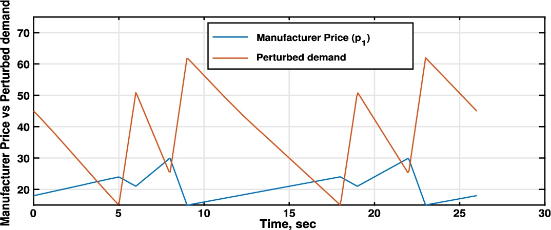
Fig. 2
Riccati differential equation player 1 (manufacturer).
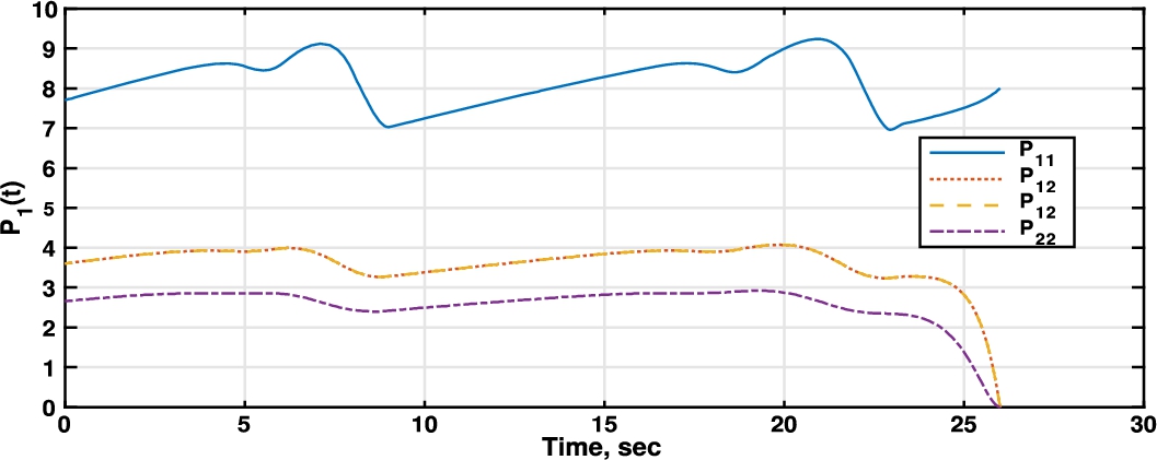
Fig. 3
Riccati differential equation player 2 (retailer).
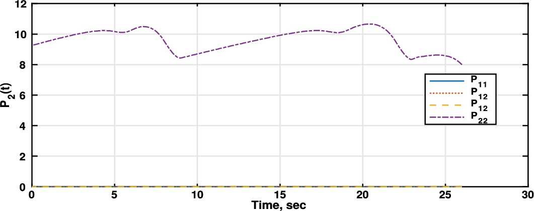
Fig. 4
Comparison between manufacturer produced units (
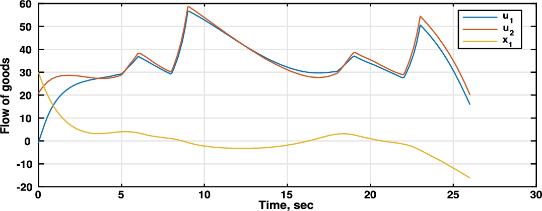
According to the game equations (1) and (2),
Also, since there are no restrictions for the states of a given stage in the chain we can see that, at times, we are going to have negative values for this variable. For example, between
Fig. 5
Comparison between retailer bought units (
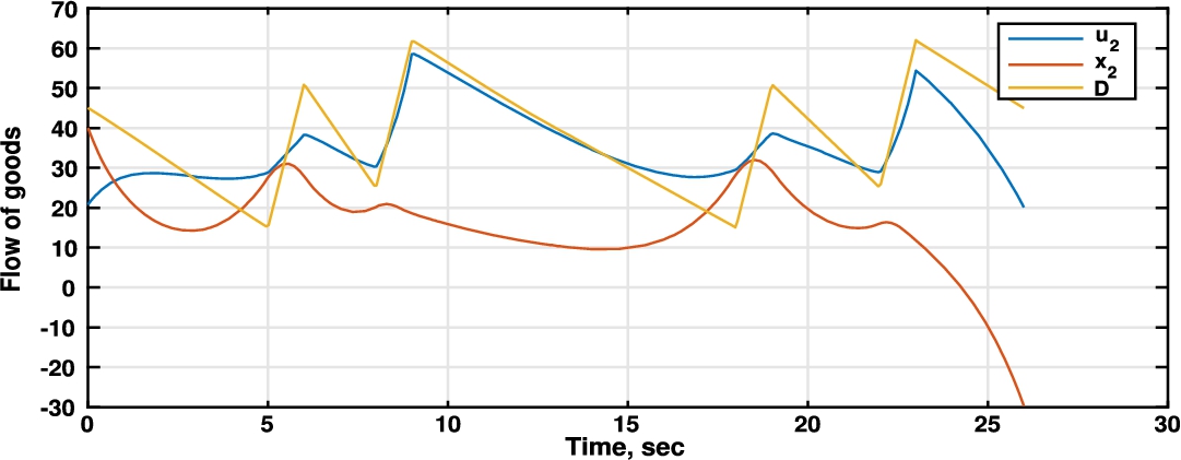
On the other hand, Fig. 5 shows the behaviour of the retailer’s dynamics through the time horizon. We can appreciate that the strategy followed by the retailer differs from the manufacturer in that the retailer uses inventory to face demand uncertainties. The retailer is considering the worst case of any perturbation on demand, but stock units are kept up to the minimum. The decisions at the end of the planning horizon are perturbed by the finite time horizon condition. For that reason the planning horizon was extended to two years in order to avoid such perturbations in the first year.
6Conclusions
We found the Nash equilibrium control function of an N players differential game affected by an
1. When we have a finite time horizon. In this case we assume the matrices involved in the performance function are time dependent.
2. When we have an infinite time horizon. In this case we assume the matrices involved in the performance function are constant with respect to the time, and there are only temporal dependence of the uncertainty function, the state function, and an affine term of the constraint given by the linear differential equation.
Both problems are solved in this work using different methods.
Appendices
A
AAppendix
Proof.
Proof of Theorem 3. To start the proof we find
(37)
(38)
(39)
(40)
(41)
(42)
Substituting (41) and (42) into (39), expanding, and grouping terms of the form
(43)
(44)
Proof.
Proof of Theorem 4. To develop the proof of this theorem let us suppose there exists an “energetic function”
(45)
Let
(46)
(47)
(48)
(49)
(50)
(51)
(52)
In (52) since
(53)
(54)
From the assumptions of equations (24)–(30), this is
(55)
Acknowledgements
The authors appreciate the used suggestions made by the anonymous referee that have helped to improve the quality of the article.
References
1 | Aliyu, M.D.S. ((2011) ). Nonlinear ℋ∞ Control, Hamiltonian sYSTEMS and Hamiltonian–Jacobi Equations. CRC Press, Boca Raton Fl. |
2 | Başar, T., Bernhard, P. ((2008) ). H∞-Optimal Control and Related Minimax Design Problems: A Dynamic Game Approach, 2nd ed. Birkhäuser. |
3 | Başar, T., Olsder, G.J. ((1999) ). Dynamic Noncooperative Game Theory 2nd ed. Classics in Applied Mathematics, Vol. 23: . SIAM. |
4 | Chen, H., Scherer, C.W., Allgöwer, F. ((1997) ). A game theoretic approach to nonlinear robust receding horizon control of constrained systems. In: Proceedings of the American Control Conference, Vol. 5: . American Automatic Control Council, pp. 3073–3077. |
5 | Chen, X., Zhou, K. ((2001) ). Multiobjective
|
6 | Dockner, E.J., Jørgensen, S., Long, N.V., Sorger, G. ((2000) ). Differential Games in Economics and Management Science. Cambridge University Press. |
7 | Engwerda, J. ((2005) ). LQ Dynamic Optimization and Differential Games. Wiley. |
8 | Engwerda, J.C. ((2017) ). Robust open-loop Nash equilibria in the noncooperative LQ game revisited. Optimal Control Applications & Methods, 38: (5), 795–813. |
9 | Fattorini, H.O. ((1999) ). Infinite-Dimensional Optimization and Control Theory. Encyclopedia of Mathematics and Its Applications, Vol. 62: . Cambridge University Press. |
10 | Friedman, A. ((1971) ). Differential Games. Pure and Applied Mathematics, Vol. XXV: . Wiley. |
11 | Jank, G., Kun, G. ((2002) ). Optimal control of disturbed linear-quadratic differential games. European Journal of Control, 8: (2), 152–162. |
12 | Jiménez-Lizárraga, M., Poznyak, A. ((2007) ). Robust Nash equilibrium in multi-model LQ differential games: analysis and extraproximal numerical procedure. Optimal Control Applications and Methods, 28: (2), 117–141. |
13 | Jørgensen, S. ((1986) ). Optimal production, purchasing and pricing: a differential game approach. European Journal of Operational Research, 24: (1), 64–76. |
14 | Jungers, M., Castelan, E.B., de Pieri, E.R., Abou-Kandil, H. ((2008) ). Bounded Nash type controls for uncertain linear systems. Automatica. A Journal of IFAC, 44: (7), 1874–1879. |
15 | Poznyak, A.S. ((2008) ). Advanced Mathematical Tools for Automatic Control Engineers, Vol. 1: Deterministic Techniques. Elsevier. |
16 | van den Broek, W.A., Engwerda, J.C., Schumacher, J.M. ((2003) ). Robust equilibria in indefinite linear-quadratic differential games. Journal of Optimization Theory and Applications, 119: (3), 565–595. |
17 | Yong, J., Zhou, X.Y. ((1999) ). Stochastic Controls: Hamiltonian Systems and HJB Equations. Applications of Mathematics, Stochastic Modelling and Applied Probability, Vol. 43: . Springer. |


