
Series with Binomial-Like Coefficients for Evaluation and 3D Visualization of Zeta Functions
Abstract
In this paper, we continue the study of efficient algorithms for the computation of zeta functions on the complex plane, extending works of Coffey, Šleževičienė and Vepštas. We prove a central limit theorem for the coefficients of the series with binomial-like coefficients used for evaluation of the Riemann zeta function and establish the rate of convergence to the limiting distribution. An asymptotic expression is derived for the coefficients of the series. We discuss the computational complexity and numerical aspects of the implementation of the algorithm. In the last part of the paper we present our results on 3D visualizations of zeta functions, based on series with binomial-like coefficients. 3D visualizations illustrate underlying structures of surfaces and 3D curves associated with zeta functions.
1Introduction
Zeta functions are very important, playing a pivotal role in the analytic number theory. Properties of zeta functions are essential in the distribution of primes. Prime numbers, in turn, have a broad spectrum of applications, ranging from quantum mechanics to information security (e.g. RSA and the Diffie–Hellman key exchange algorithms or elliptic-curve cryptography). Investigating zeta functions numerically, one needs an algorithm enabling to effectively compute numerous values over the complex plane, not only in the critical strip or on the critical line.
In this paper, we continue the study of efficient algorithms for the computation of zeta functions, extending works of Borwein (2000), Šleževičienė (2004), Vepštas (2008) and Coffey (2009). These algorithms allow the computation of zeta functions over the complex plane. The idea of the method comes from the alternating series convergence and properties of Chebyshev polynomials. The algorithm is nearly optimal in the sense that there is no sequence of n-term exponential polynomials that can converge to a zeta function very much faster than those of the algorithm (see, e.g. Theorem 3.1 in Borwein, 2000, Theorem 5 in Šleževičienė, 2004). The algorithm steps aside for the Riemann–Siegel formula based algorithms (Arias de Reyna, 2011) for computations concerning zeroes on the critical line, where multiple low precision evaluations are required. However, it is more efficient than Euler–Maclaurin based algorithms for arbitrary precision computations (note that the Riemann–Siegel formula permits to approximate
In the present study, we develop a modification of a globally convergent series for the Riemann zeta function and establish a limit theorem for coefficients of the modified series. We specify the rate of convergence to the limiting distribution, identify the error term and discuss computational complexity. The algorithm is applied to produce 3D visualizations, illustrating underlying structures of surfaces and 3D curves associated with zeta functions.
The paper is organized as follows. The first part is the introduction. In the second part, we introduce a modification of Lerch’s series. In the auxiliary third part, we establish double ordinary and double semi-exponential generating functions for coefficients of the modified series. The proof of the validity of the modification is presented in the fourth section. In the fifth part of the research, we establish analytic expressions of coefficients of the series. In the sixth section, we establish a limit theorem for coefficients and specify the rate of convergence to the limiting distribution. In the seventh section, we prove a theorem for the error term of the series and consider the computational complexity of the method. The numerical aspects of the technique are discussed in the eighth part of the paper. The ninth section of the study is devoted to 3D visualizations of zeta functions and the Riemann hypothesis.
Throughout this paper, we denote by
2Series with Binomial-Like Coefficients
Let
Theorem 1.
For
(1)
(2)
(3)
Table 1
Numbers
| 0 | 1 | 2 | 3 | 4 | 5 | … | |
| 0 | 1 | 0 | 0 | 0 | 0 | 0 | … |
| 1 | 3 | 1 | 0 | 0 | 0 | 0 | … |
| 2 | 7 | 4 | 1 | 0 | 0 | 0 | … |
| 3 | 15 | 11 | 5 | 1 | 0 | 0 | … |
| 4 | 31 | 26 | 16 | 6 | 1 | 0 | … |
| 5 | 63 | 57 | 42 | 22 | 7 | 1 | … |
| … | … | … | … | … | … | … | … |
It is significant to note that though the partial difference equation (3) bears a close resemblance to the partial difference equation of the binomial coefficients, coefficients
The series (1) is a modification of the globally convergent series for the Riemann zeta function, first given by Lerch (1897),
(4)
3Generating Functions of the Coefficients of the Series
In this section we establish the double ordinary generating function
(5)
(6)
Lemma 1.
Coefficients
(7)
(8)
Proof.
Let us consider the formal series (5) of the double ordinary generating function (note that
Next, take a look at the formal series (6) of the double semi-exponential generating function,
Lemma 2.
Coefficients
(9)
(10)
Proof.
Let us take the double ordinary generating function (5). Substituting the expression (3) into the generating function, we get
(11)
Next, turn to the double semi-exponential generating function (6). Substituting the recurrent expression (3) into the generating function, we have that
4Analytic Expressions of the Coefficients of the Series
The recurrent formula (3) is often inconvenient in practical computations, thus it is purposeful to seek an analytic expression or an asymptotic expansion. We may view (3) as a partial difference equation with constant coefficients. In this section we will establish analytic expressions for the coefficients
Lemma 3.
The following analytic expressions are equivalent:
(12)
Proof.
Formal Taylor series in two variables for generating functions
Next, using proposition (ii) of Lemma 2, we get
(13)
The third statement of the lemma follows from the formula for the distribution of the probabilities in the Bernoulli scheme (see (19) on page 27 in Bolshev and Smirnov, 1983),
Remark 1.
The first and the second statements of Lemma 3 also can be proved by the direct application of the definition (3) (or by induction). However, these approaches do not reveal the underlying nature of the numbers
Now we can proceed with the proof of Theorem 1.
5Proof of Theorem 1
Proof.
Consider Lerch’s series (4) for the Riemann zeta function
6Limit Theorem for the Coefficients of the Series and the Rate of Convergence to the Limiting Distribution
We will use Hwang’s result on convergence rates in central limit theorems for combinatorial structures (see Theorem 7 and Corollary 2 in Section 4 in Hwang, 1998) to establish the limit theorem for
Theorem 2.
(See Hwang, 1998.) Let
(14)
Let us formulate a central limit theorem.
Lemma 4.
Suppose that
(15)
(16)
(17)
(18)
Proof.
Let us consider the moment generating function of the random variable
Next, let us examine the probability generating function of the random variable
(19)
Now we can formulate the central limit theorem for the coefficients
Proof.
Note that the cumulative distribution function of the random variable
7Error Term of the Series and the Computational Complexity
Let us investigate the error term of the series (1).
Theorem 4.
For
(21)
(22)
Proof.
By (2.3) of Algorithm 1 in Borwein (2000), the error term of the series equals
(23)
(24)
(25)
(26)
(27)
(28)
(29)
Remark 2.
For
(30)
(31)
(32)
(33)
8Numerical Aspects
Apart from a certain theoretical interest, the representation (20) of
(34)
The algorithm requires a number of terms n (32) to compute
Naturally, a direct application of the recurrent equation (3) (if values are stored) is faster, compared to straightforward repeated recalculations. However, this storage-intensive approach is unattractive (note order of
Table 2
Time required to achieve six decimal digits of accuracy, [sec].
| Alg. mod. |
|
| ||||
|
|
|
|
|
|
| |
| RE | 0.38 | 0.36 | 0.31 | 293.55 | 298.09 | 290.84 |
| BF | 0.14 | 0.14 | 0.13 | 12.20 | 12.47 | 11.58 |
| NA | 0.05 | 0.05 | 0.05 | 4.16 | 4.41 | 4.07 |
| RE
| 0.18 | 0.18 | 0.16 | 90.20 | 97.51 | 87.74 |
| BF
| 0.10 | 0.10 | 0.09 | 6.63 | 6.96 | 6.57 |
| NA
| 0.04 | 0.04 | 0.04 | 2.37 | 2.53 | 2.38 |
In Table 2 we compare the performance of six modifications of the algorithm for the computation of the Riemann zeta function, based on the series with binomial-like coefficients. Namely,
• Recurrent Expression (RE). The coefficients of the series (21) are calculated using the recurrent expression (3). The number of terms n in the sum is obtained by applying the approximation (33).
• Beta function (BF). The coefficients of the series (21) are calculated using the regularized incomplete beta function (see (iii) of Lemma 3). The number of terms n in the sum is obtained by applying the approximation (33).
• Normal approximation (NA). The coefficients of the series (21) are calculated using the asymptotic (20). The standard normal cumulative distribution function is approximated with a 16-digit precision using the fast computation algorithm proposed by (West, 2005). The number of terms n in the sum is obtained by applying the approximation (33).
• Recurrent Expression with
• Beta function with
• Normal approximation with
Let us denote the sets for σ:
We can see that asymptotic-based modifications are 2–3 times faster than beta-based modifications, while recurrence-based modifications have proved too computationally demanding for intensive practical use. Note that C++ version of the program would bring more substantial benefits in speedup (cf. Belovas and Sakalauskas, 2018). Numerical experiments have shown that processing 3D visualizations of surfaces and curves, associated with zeta functions, the performance comparable with Zetafast algorithm (Fischer, 2017), while the specified accuracy level does not exceed six decimal digits of accuracy and the coefficients
93D visualizations of Zeta Functios
Visualizing a complex function of a complex variable
The first two figures present two examples of 3D visualizations of the pattern of the allocation of non-trivial zeros of the Riemann zeta function. Figure 1 illustrates the initial allocation (for
Fig. 1
Zeroes,
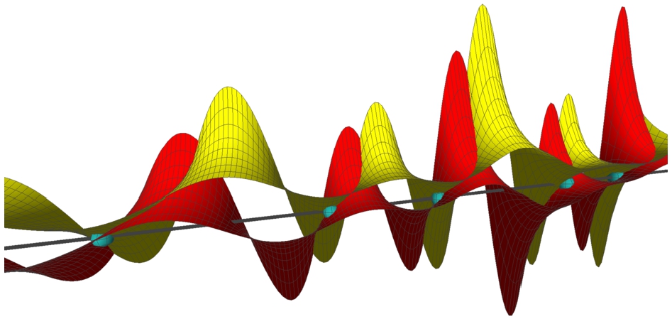
Figure 2 visualizes a segment of the pattern, containing 91–100th non-trivial zeroes of the Riemann zeta function (for
Fig. 2
Zeroes,
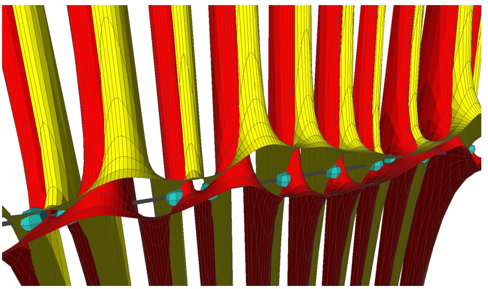
Fig. 3
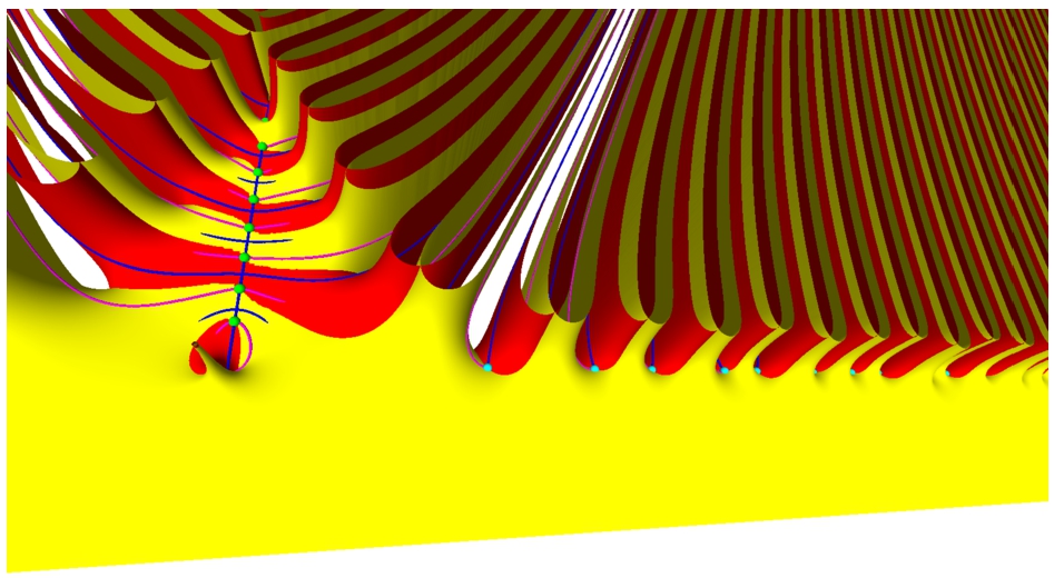
Figure 3 shows numerous ridges shaped by the real (yellow) and the imaginary (red) surfaces of the Riemann zeta function (for
Figure 4 extends the visualization of the previous illustration, demonstrating a 2D pattern of intersections of the real and the imaginary surfaces of the Riemann zeta function with the complex plane. Non-trivial zeros are indicated by small cyan balls. Trivial zeros are indicated by green ones.
Fig. 4
2D curves corresponding the intersections of
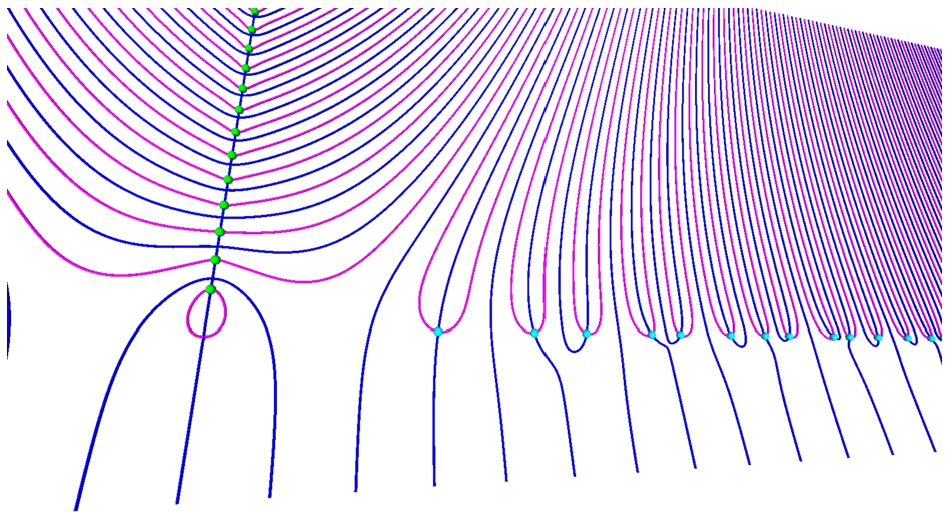
Figure 5 shows a pattern of intersections of the real (yellow) and the imaginary (red) surfaces of the Riemann zeta function (for
Fig. 5
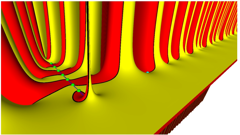
Figure 6 extends the visualization of the previous illustration, revealing a knot of 3D curves corresponding the intersections of the surfaces, while the surfaces themselves are not shown.
Fig. 6
3D curves corresponding the intersections of
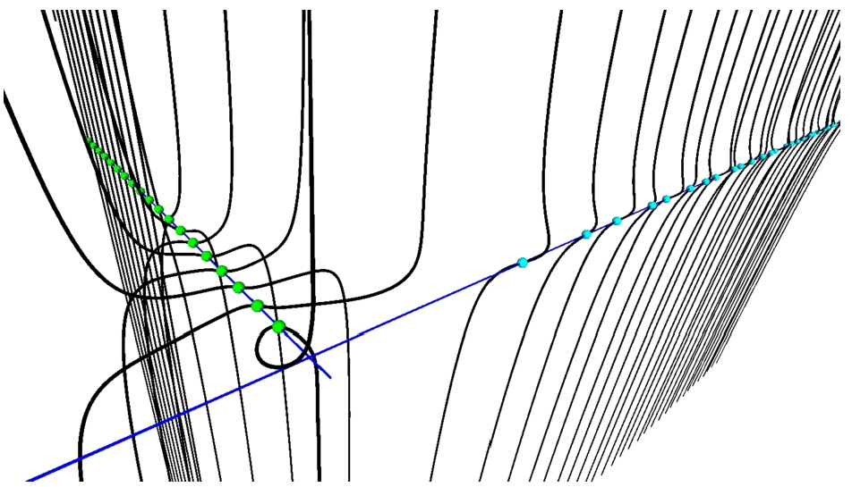
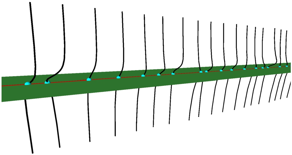
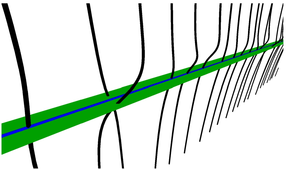
Figure 7 presents a visualization of the Riemann hypothesis. We can see ribs, formed by the intersections of the real and the imaginary surfaces of the Riemann zeta function, going through the critical line (red) in the critical strip
Fig. 7
3D curves corresponding the intersections of
The next visualizations present a counterexample to a “generalized Riemann hypothesis”. Let us consider the linear combination of the Riemann zeta function and the Dirichlet L-function (cf. Garunkštis and Šimėnas, 2015),
(35)
Let us go with
Fig. 8
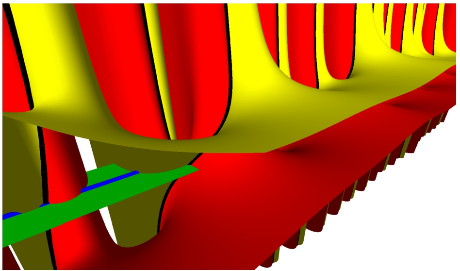
Figure 9 demonstrates the intersections of 3D curves (corresponding the intersections of the real and the imaginary surfaces of the linear combination (35)) with the complex plane in the critical strip
Fig. 9
3D curves corresponding the intersections of
References
1 | Arias de Reyna, J. ((2011) ). High precision computation of Riemann’s zeta function by the Riemann–Siegel formula. Mathematics of Computation, 80: (274), 995–1009. https://doi.org/10.1090/S0025-5718-2010-02426-3. |
2 | Belovas, I. ((2019) a). A central limit theorem for coefficients of the modified Borwein method for the calculation of the Riemann zeta-function. Lithuanian Mathematical Journal, 59: (1), 17–23. https://doi.org/10.1007/s10986-019-09421-4. |
3 | Belovas, I. ((2019) b). A local limit theorem for coefficients of modified Borwein’s method. Glasnik Matematički, 54: (74), 1–9. https://doi.org/10.3336/gm.54.1.01. |
4 | Belovas, I., Sakalauskas, L. ((2018) ). Limit theorems for the coefficients of the modified Borwein method for the calculation of the Riemann zeta-function values. Colloquium Mathematicum, 151: (2), 217–227. https://doi.org/10.4064/cm7086-2-2017. |
5 | Bolshev, L.N., Smirnov, N.V. ((1983) ). Tablitsy matematicheskoj statistiki. Nauka, Moscow (in Russian). |
6 | Borwein, P. ((2000) ). An efficient algorithm for the Riemann zeta function. In: Constructive, Experimental, and Nonlinear Analysis, Limoges, 1999, CMS Conference Proceedings,Vol. 27: . American Mathematical Society, Providence, RI, pp. 29–34. |
7 | Borwein, J.M., Bradley, D.M., Crandall, R.E. ((2000) ). Computational strategies for the Riemann zeta function. Journal of Computational and Applied Mathematics, 121: (1–2), 247–296. https://doi.org/10.1016/S0377-0427(00)00336-8. |
8 | Coffey, M.W. ((2009) ). An efficient algorithm for the Hurwitz zeta and related functions. Journal of Computational and Applied Mathematics, 225: (2), 338–346. https://doi.org/10.1016/j.cam.2008.07.040. |
9 | Fischer, K. (2017). The Zetafast algorithm for computing zeta functions. arXiv:1703.01414. |
10 | Garunkštis, R., Šimėnas, R. ((2015) ). On the Speiser equivalent for the Riemann hypothesis. European Journal of Mathematics, 1: (2), 337–350. https://doi.org/10.1007/s40879-014-0033-1. |
11 | Gradshteyn, I.S., Ryzhik, I.M. ((2014) ). Table of Integrals, Series, and Products (8th ed.). Academic Press. |
12 | Hwang, H.-K. ((1998) ). On convergence rates in the central limit theorems for combinatorial structures. European Journal of Combinatorics, 19: (3), 329–343. https://doi.org/10.1006/eujc.1997.0179. |
13 | Kaczorowski, J., Kulas, M. ((2007) ). On the non-trivial zeros off the critical line for L-functions from the extended Selberg class. Monatshefte für Mathematik, 150: (3), 217–232. https://doi.org/10.1007/s00605-006-0412-x. |
14 | Lerch, M. ((1897) ). Expressions nouvelles de la constante d’Euler, Věstník Královské české společnosti náuk. Tř. mathematicko-přírodovědecká, 42: , 1–5. |
15 | Šleževičienė, R. ((2004) ). An efficient algorithm for computing Dirichlet L-functions. Journal Integral Transforms and Special Functions, 15: (6), 513–522. https://doi.org/10.1080/1065246042000272072. |
16 | Stopple, J. ((2017) ). Lehmer pairs revisited. Experimental Mathematics, 26: (1), 45–53. https://doi.org/10.1080/10586458.2015.1107870. |
17 | Vepštas, L. ((2008) ). An efficient algorithm for accelerating the convergence of oscillatory series, useful for computing the polylogarithm and Hurwitz zeta functions. Numerical Algorithms, 47: (3), 211–252. https://doi.org/10.1007/s11075-007-9153-8. |
18 | West, G. (2005). Better approximations to cumulative normal functions. Wilmott Magazine, 70–76. |


