
Perceptual Autoencoder for Compressive Sensing Image Reconstruction
Abstract
This paper presents a non-iterative deep learning approach to compressive sensing (CS) image reconstruction using a convolutional autoencoder and a residual learning network. An efficient measurement design is proposed in order to enable training of the compressive sensing models on normalized and mean-centred measurements, along with a practical network initialization method based on principal component analysis (PCA). Finally, perceptual residual learning is proposed in order to obtain semantically informative image reconstructions along with high pixel-wise reconstruction accuracy at low measurement rates.
1Introduction
Compressive sensing (CS) is a signal processing technique that enables accurate signal recovery from an incomplete set of measurements (Candes and Tao, 2006; Baraniuk, 2007; Duarte and Eldar, 2011; Duarte and Baraniuk, 2012):
(1)
The CS reconstruction process can be observed as a linear inverse problem that occurs in numerous image processing tasks such as inpainting (Bertalmio et al., 2000; Bugeau et al., 2010), super-resolution (Yang et al., 2010; Dong et al., 2016), and denoising (Elad and Aharon, 2006). In order to reconstruct the signal
(2)
(3)
After being successfully applied to numerous previously mentioned image processing tasks, machine learning methods started to gain more interest in the area of CS (Mousavi et al., 2015; Mousavi and Baraniuk, 2017; Mousavi et al., 2017; Kulkarni et al., 2016; Hantao et al., 2019; Lohit et al., 2018). Novel CS reconstruction algorithms based on deep neural networks have recently been proposed, and they represent a non-iterative, fast and efficient alternative to the traditional CS reconstruction algorithms.
2Related Work
A deep learning framework based on the stacked denoising autoencoder (SDA) has been proposed in Mousavi et al. (2015) and it represents pioneer work in the area of CS reconstruction using the learning-based approach. The main drawback of the SDA approach is that the network consists of fully-connected layers, which means that all units in two consecutive layers are connected to each other. Thus, as the signal size increases, so does the computational complexity of the neural network. Authors present an extension of their previous work in Mousavi and Baraniuk (2017) and Mousavi et al. (2017). The DeepInverse network proposed in Mousavi and Baraniuk (2017) solves the image dimensionality problem by using the adjoint operator
In this paper, we propose an efficient deep learning model for CS acquisition and reconstruction. Our model is based on a fully convolutional autoencoder with a residual network. Fully convolutional architecture alleviates the signal dimensionality problems that occur in the full-connected network design (Mousavi et al., 2015). Disadvantage of using the fully convolutional architecture is that it is not directly applicable to certain imaging modalities where the measurements correspond to the whole signal, and one cannot perform measurements in a blockwise manner. In contrast to Mousavi et al. (2017) where the authors propose to learn a non-linear measurement operator in their DeepCodec network, we use a linear encoding part while the non-linearities are introduced only into the residual learning network. Motivation for this is to ensure that the learned measurement operator is implementable in the real-world CS measurement systems which are mostly linear. The residual network improves the initial image reconstruction and removes eventual reconstruction artifacts.
Although it is well known that normalization of the training data significantly speeds up the training procedure (Ioffe and Szegedy, 2015), applying the measurement normalization in the learning-based CS is not straightforward. In order to normalize and mean-centre the CS measurements, measurement process has to be redesigned. Mean values of the observed image blocks have to be known in order to perform mean-centring and normalization. Therefore, we dedicate a single measurement vector to measure the mean value of the observed image block. The rest of the measurement matrix is optimized in the training process. Input to the decoding part of the proposed model are mean-centred measurements, and the decoding process results in mean-centred image reconstruction. Mean value for the observed block is then added to the initial image estimate to obtain the final image reconstruction. Without the proposed modifications of the measurement process, performing reconstruction on normalized measurements would not be feasible. As expected, we show that the measurement normalization process speeds up the convergence of the network significantly.
Furthermore, we discuss the connection between the linear autoencoder network and principal component analysis (PCA). Based on our observations, an efficient method for initialization of the network weights is proposed. The proposed method serves as a bootstraping step in the network training procedure. Instead of initializing the model using random weights, we propose to use an educated guess for the initial weights by using the PCA initialization method.
Finally, we introduce perceptual loss in the residual network training in order to improve the reconstructions at extremely low measurement rates. Experimental results obtained using the proposed model show improvements in terms of the reconstruction quality.
The paper is organized as follows: in Section 3.1, convolutional autoencoder for CS image reconstruction is proposed. Section 3.2 and Section 3.4 offer a discussion on the measurement matrix optimality and efficient network initialization. Section 3.3 introduces the normalized measurement process. Finally, perceptual residual learning is introduced in Section 3.5 in order to improve the image reconstructions obtained by the autoencoder. Section 4 presents the main results with discussion, while Section 6 offers the conclusion.
3Proposed Architecture for the CS Model
3.1Convolutional Autoencoder
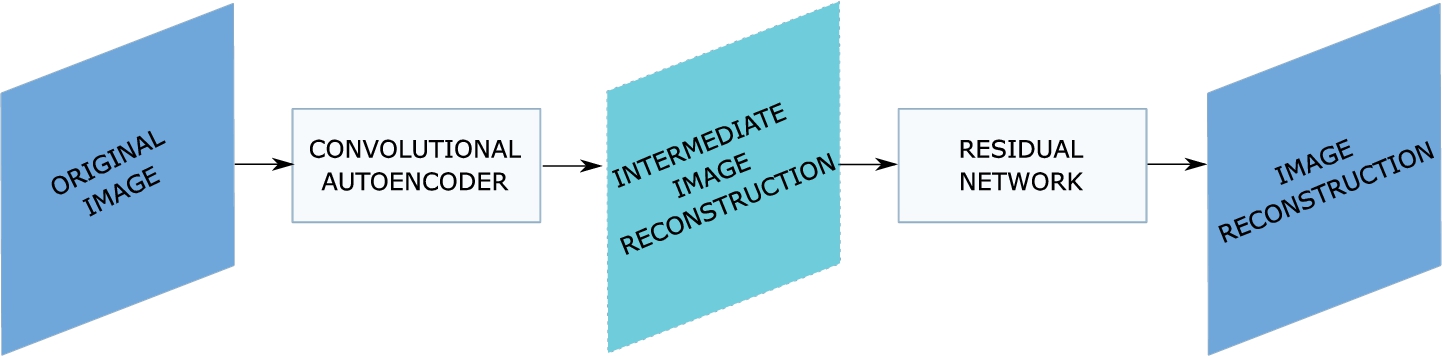
The encoding part of the proposed shallow autoencoder network performs the CS measurement process on an input image, while the decoding part models the CS reconstruction process and reconstructs the input image from the low-dimensional measurement space (Fig. 1).
Fig. 1
Proposed design of the CS image reconstruction model. The convolutional autoencoder learns the end-to-end CS mapping. The encoder performs synthetic measurements on the input image, transforming it into the low-dimensional measurement space. The decoding part learns the optimal inverse mapping from the low-dimensional measurements into the intermediate image reconstruction. The residual network additionally improves the initial image reconstruction.
In the traditional CS measurement process, an image is vectorized to form a one-dimensional vector
(4)
In this paper, a linear convolutional layer performs decimated convolution, as in Eq. (5), in order to obtain the measurements. Convolution can be used as an extension of the inner product in which the inner product is computed repeatedly over the image space.
(5)
The CS reconstruction process is modelled using a transposed convolution (Dumoulin and Visin, 2016), and the decoding part of the autoencoder is trained to learn the optimal pseudo-inverse linear mapping operator
Fig. 2
Creating a set of measurement filters from the measurement matrix. Row vector
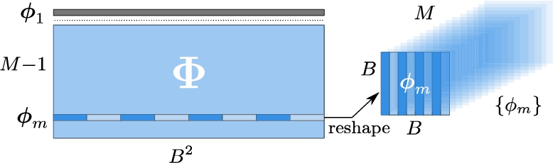
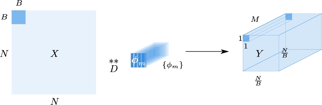
Fig. 3
Visualization of the measurement process using decimated 2D convolution. Block x of size
3.2Predefined vs. Adaptive Measurement Matrix
There are two basic approaches for the measurement matrix design. An arbitrary measurement matrix Φ can be used in the measurement process to obtain measurements
Alternatively, the optimal measurement matrix can be inferred from the training data. Such a matrix better adapts to the dataset and preserves more information in the measurements, resulting in better reconstruction results. In our proposal, we optimize the encoding part of the autoencoder to learn the optimal linear measurement matrix Φ from the training dataset. In the experimental section, we show the effect of the measurement matrix choice on the reconstruction results.
3.3Network Training Using Normalized Measurements
Training neural networks on normalized, mean-centred data became standard in all areas of machine learning (Ioffe and Szegedy, 2015). It is well known that such practice significantly reduces the training time, but the application to the learning based CS is not straightforward. The measurement process needs to be redesigned in order to obtain normalized and mean-centred measurements, since the mean value of the observed signal has to be measured during the CS acquisition process. In this section, we present an efficient measurement process which enables the direct application of data normalization techniques, which is in contrast with the previous work in this area.
In order to measure the mean value
(6)
(7)
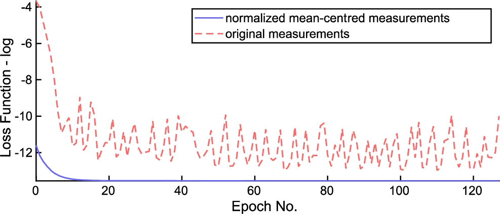
Training the neural network on non-mean-centred data has undesirable consequences. If the data coming into a neuron is always positive (e.q.
Fig. 4
Training loss function. Normalized mean-centred measurements vs. original measurements. Notice the zig-zagging in the loss function when using non-centred measurement data. Loss functions are visualized on the log scale.
3.4Efficient Method for Network Initialization
In Lohit et al. (2018) and Du et al. (2019), the authors optimize the linear encoder in order to infer the optimal measurement matrix for each measurement rate r. In Baldi and Hornik (1989), it has been shown that the linear autoencoder with the mean squared error (MSE) loss converges to a unique minimum corresponding to the projection onto the subspace generated by the first principal component vectors of the covariance matrix obtained using the principal component analysis (PCA). Thus, it is sub-optimal to retrain the model for each measurement rate r.
Instead, we propose an efficient initialization method for the deep learning CS models based on the observation from Baldi and Hornik (1989). Principal component analysis (PCA) is an analytic method that has a widespread use in dimensionality reduction. The PCA is performed on the covariance matrix of the data vector
(8)
(9)
(10)
Thus, we propose to use the reduced eigenvector matrix
(11)
Furthermore, we propose to initialize the reconstruction part of the network using the PCA as well. The eigenvector matrix
(12)
(13)
The proposed initialization method for the network weights has several advantages. While a neural network has to be retrained in order to obtain the measurement matrix Φ for a different sub-rate r, the PCA approach outputs the whole eigenvector matrix
3.5Residual Network
As previously mentioned, the first part of the proposed network consists of a linear autoencoder. Non-linearities can be easily introduced into the measurement and reconstruction part of the network to further improve the initial reconstruction obtained by the autoencoder. In our proposal, non-linearities are only introduced into the decoding part of the network. Although there are some methods that learn a non-linear measurement operator from the data (Mousavi et al., 2017), linearity is an important property of measurement systems and we want our CS model to be realizable in real physical measurement setups like Takhar et al. (2006) and Ralašić et al. (2018).
Fig. 5
Contrast-adjusted visualization of the learned residual for several test images and for the measurement ratio
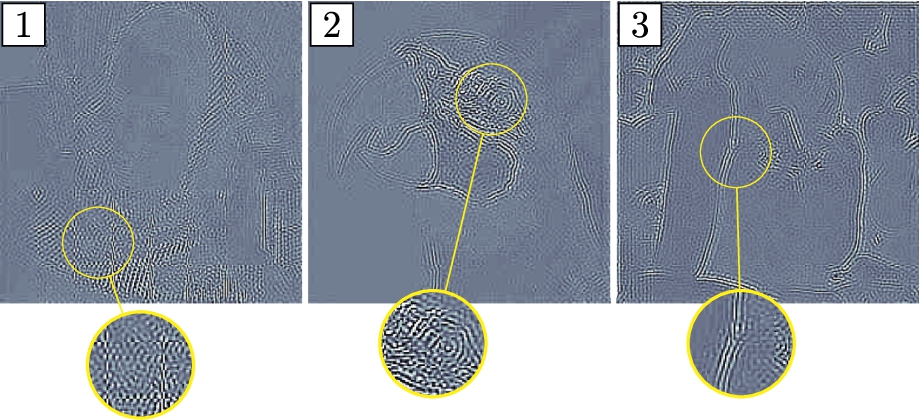
The output of the proposed convolutional autoencoder represents a preliminary reconstruction of the input image from its low-dimensional measurements. We feed the preliminary reconstruction to a residual network (He et al., 2015) that induces non-linearity and reduces potential reconstruction and blocking artifacts, and eliminates the need for an off-the-shelf denoiser such as BM3D (Dabov et al., 2009) used in the competitive methods. Figure 5 shows several examples of the estimated residual. Residual learning compensates for some of the high-frequency loss and improves the initial image reconstruction.
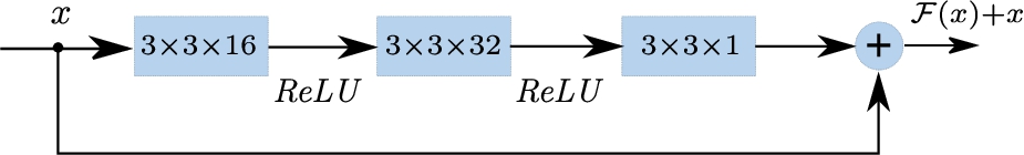
Figure 6 shows the architecture of the residual learning block used in our proposal. The residual network consists of two residual learning blocks and each residual learning block has three layers. The first layer consists of 16 convolutional filters of size
3.6Choice of the Loss Function
Reconstructing the high-frequency content in the original image (i.e. edges, texture) is problematic for the linear autoencoder, and the residual network helps to alleviate this problem. Problems occur partly due to the fact that the lower frequency content is dominant in natural images and the learned measurement filters have a low-pass character, and partly due to the choice of the loss function used for training the network. It is known that the MSE loss function yields blurry images (Kristiadi, 2019). Thus, some papers suggest using a different loss function for the network training. As an example, Lohit et al. (2018) uses the adversarial loss function in addition to Euclidean loss to obtain better and sharper reconstructions. Furthermore, Du et al. (2018) uses perceptual loss in order to achieve better reconstruction results. The authors train their model using the Euclidean loss in the latent space of the
In this paper, we fuse the per-pixel reconstruction loss in the autoencoder with the perceptual loss in latent space in the residual network. This is in contrast with Du et al. (2018), where the authors optimize the whole network using the Euclidean loss in the latent space. As a consequence, their method results in semantically informative reconstructions, but with low per-pixel accuracy. By using a combination of Euclidean and perceptual loss, we obtain semantically informative reconstructions that have high accuracy of per-pixel reconstruction resulting in higher PSNR compared to Du et al. (2018).
Fig. 6
Residual learning block. The residual learning block consists of 3 convolutional layers.
Pixel-wise Euclidean loss function for the autoencoder is defined as:
(14)
The residual part of the proposed network is trained separately from the autoencoder part using perceptual loss function
(15)
4Experiments
4.1Network Training
In this section, we discuss the details of our network training procedure. We use tensorflow (Abadi et al., 2015) deep learning framework for training and testing purposes. The training dataset is formed using uncalibrated JPEG images from the publicly available Barcelona Calibrated Images Database (Párraga et al., 2010). Our training dataset is created by extracting 1676 image patches of size
Adam optimizer (Kingma and Ba, 2015) (
We perform series of experiments to corroborate previous discussions and observations. In order to achieve a fair comparison framework, a set of 11 images (Monarch, Fingerprint, Flintstones, House, Parrot, Barbara, Boats, Cameraman, Foreman, Lena, Peppers – see TestDataset), which were used in the evaluation of the competitive methods are used for testing purposes with four different measurement sub-rates
4.2Measurement Matrix
In Section 3, we have discussed the connection between the measurement matrix learned by the linear encoder and the one obtained by performing the PCA analysis. In addition, we proposed an efficient initialization method for the network weights. In this section, we perform an experiment to show that the performance of the trained linear autoencoder is limited by the performance of the PCA method network in terms of image reconstruction quality.
Table 1
Comparison of linear autoencoder and PCA in terms of reconstruction PSNR [dB].
| PSNR [dB] | ||||
| PCA | 31.45 | 27.11 | 23.95 | 20.56 |
| Linear autoencoder | 31.39 | 27.06 | 23.92 | 20.55 |
Table 1 shows the mean reconstruction results in terms of PSNR for the standard test images. Notice that the reconstruction results are comparable. The slightly lower reconstruction performance of the linear encoder is due to the network not fully converging to the global minimum. Reconstruction results obtained by using the PCA method represent an upper boundary for the performance of the linear autoencoder network for CS image reconstruction.
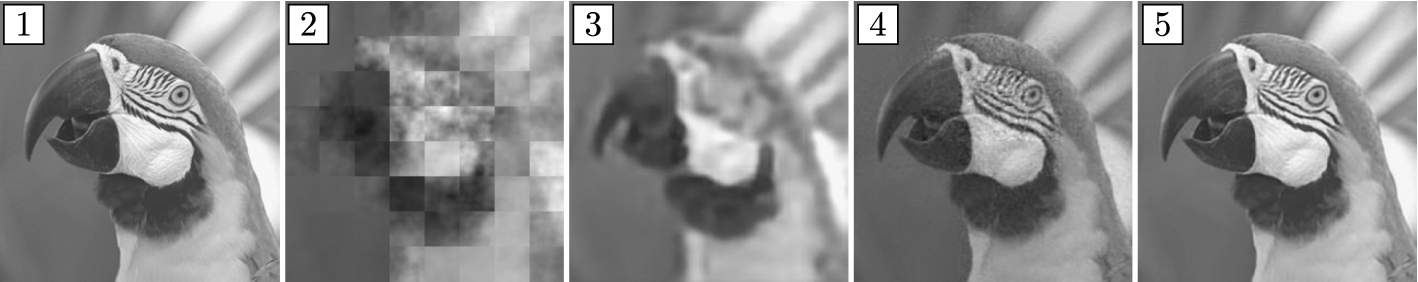
In Fig. 7, reconstruction results obtained using random Gaussian and adaptive measurement matrix for Parrot test image are shown. The reconstructions are presented for measurement rates
Fig. 7
Reconstruction results obtained using linear autoencoder for “Parrot” test image (1) and for two measurement ratios
4.3Comparison to Other Methods
In this section, we compare the proposed CS model to other state-of-the-art learning-based CS methods. To provide a fair comparison, we compare our method only to similar methods which use an adaptive linear encoding part.
We compare our method to the ImpReconNet (Lohit et al., 2018), Adp-Rec (Xie et al., 2017), FCMN (Du et al., 2019) and two variants of PCS (Du et al., 2018), namely
Table 2
Reconstruction results obtained using the learned measurement matrix. Table contains mean PSNR reconstruction results for the standard test images at different measurement rates r. Although, FCMN achieves better results in terms of PSNR, it is clearly visible from Fig. 8 that it does not preserve structural information. This is due to the fact that PSNR measures image quality on per pixel basis, which is not a relevant measure for the preservation of high-level image features.
| Mean PSNR [dB] for different methods | ||||
| ImpReconNet (Euc) (Lohit et al., 2018) | 26.59 | 25.51 | 23.14 | 19.44 |
| ImpReconNet (Euc + Adv) (Lohit et al., 2018) | 30.53 | 26.47 | 22.98 | 19.06 |
| Adp-Rec (Xie et al., 2017) | 30.80 | 27.53 | – | 20.33 |
| FCMN (Du et al., 2019) | 32.67 | 28.30 | 23.87 | 21.27 |
| – | – | 19.38 | 18.30 | |
| – | – | 16.72 | 16.80 | |
| Proposed method | 32.00 | 26.36 | 23.67 | 20.51 |
Fig. 8
Reconstruction results for “Fingerprint” test image and for measurement rate
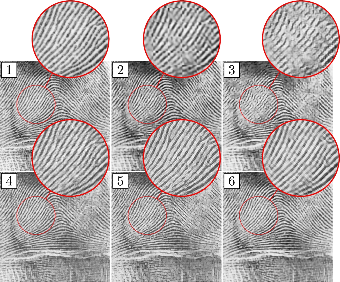
On one hand, FCMN and ImpReconNet yield similar results in terms of PSNR compared to our method (see Table 2), while on the other hand the aforementioned methods do not preserve structural and high level semantic information. The two PCS methods preserve structural information, but yield images that contain significant amount of noise when observed on pixel-wise level. Our method benefits from the combination of pixel-wise Euclidean loss in image space and the Euclidean loss in the latent space of the
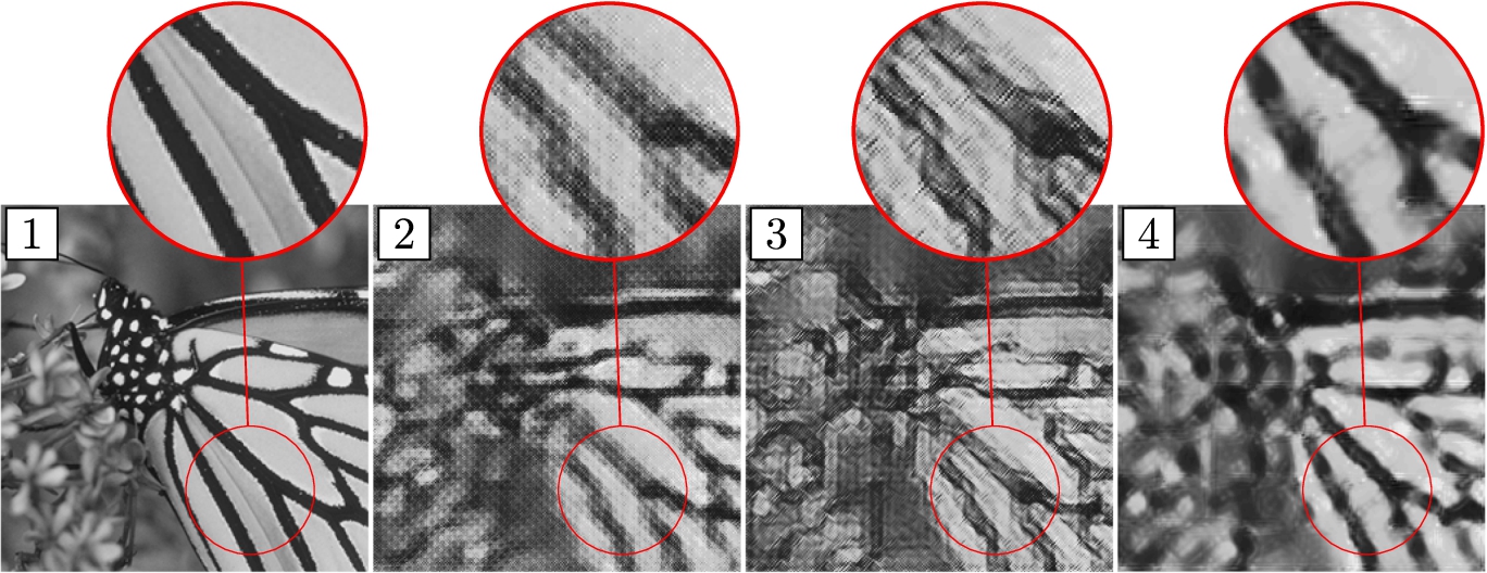
Fig. 9
Reconstruction results for “Monarch” test image and for measurement rate
5Discussion
Iterative nature and high computational complexity present the main drawbacks of the traditional CS reconstruction algorithms. Learning based methods for the CS image reconstruction present an efficient alternative to the traditional approach. Average per-image reconstruction time for a set of images with size
Better performance of the learning based methods in the reconstruction phase comes at an increased cost in the training phase. In order to learn the optimal measurement and reconstruction operators, learning based methods require an offline training procedure with a relatively large training dataset. Since learning based methods are data driven, they are also data dependent. Thus, if the statistical distribution of the training dataset significantly differs from the testing data, the performance of the learning based methods will be influenced. Finally, convolutional block image processing is not applicable in imaging modalities where the measurements correspond to the whole signal, and one cannot divide the signal into smaller blocks.
6Conclusion
In this paper, we proposed a convolutional autoencoder architecture for the image compressive sensing reconstruction, which represents a non-iterative and extremely fast alternative to the traditional sparse optimization algorithms. In contrast with other learning based methods, we designed a measurement process which enables the model to be trained on normalized, mean-centred measurements which results in a significant speedup of the neural network convergence. Moreover, we proposed an efficient initialization method for the autoencoder network weights based on the connection between the learning-based CS approach and the principal component analysis. The residual learning network was used to further improve the initial reconstruction obtained by the autoencoder.
A combination of a pixel-wise Euclidean loss function for the autoencoder network training along with a Euclidean loss function in the latent space of the
References
1 | Abadi, M., Agarwal, A., Barham, P., Brevdo, E., Chen, Z., Citro, C., Corrado, G.S., Davis, A., Dean, J., Devin, M., Ghemawat I, S., Goodfellow, Harp, A., Irving, G., Isard, M., Jia, Y., Jozefowicz, R., Kaiser, L., Kudlur, M., Levenberg, J., Mané, D., Monga, R., Moore, S., Murray, D., Olah, C., Schuster, M., Shlens, J., Steiner, B., Sutskever, I., Talwar, K., Tucker, P., Vanhoucke, V., Vasudevan, V., Viégas, F., Vinyals, O., Warden, P., Wattenberg, M., Wicke, M., Yu, Y., Zheng, X. (2015). TensorFlow: Large-Scale Machine Learning on Heterogeneous Systems. Online: https://www.tensorflow.org/. |
2 | Baldi, P., Hornik, K. ((1989) ). Neural networks and principal component analysis: learning from examples without local minima. Neural Networks, 2: , 53–58. |
3 | Baraniuk, R.G. ((2007) ). Compressive sensing [lecture notes]. IEEE Signal Processing Magazine, 24: , 118–121. |
4 | Beck, A., Teboulle, M. ((2009) ). A fast iterative shrinkage-thresholding algorithm for linear inverse problems. SIAM Journal on Imaging Sciences, 2: , 183–202. |
5 | Becker, S., Bobin, J., Candès, E.J. ((2011) ). NESTA: a fast and accurate first-order method for sparse recovery. SIAM Journal on Imaging Sciences, 4: , 1–39. |
6 | Bertalmio, M., Sapiro, G., Caselles, V., Ballester, C. ((2000) ). Image inpainting. In: Proceedings of the 27th Annual Conference on Computer Graphics and Interactive Techniqus. ACM Press/Addison-Wesley Publishing Co., pp. 417–424. |
7 | Bugeau, A., Bertalmio, M., Caselles, V., Sapiro, G. ((2010) ). A comprehensive framework for image inpainting. IEEE Transactions on Image Processing, 19: , 2634–2645. |
8 | Candes, E.J., Tao, T. ((2006) ). Near-optimal signal recovery from random projections: universal encoding strategies? IEEE Transactions on Information Theory, 52: , 5406–5425. |
9 | Dabov, K., Foi, A., Katkovnik, V., Egiazarian, K. ((2009) ). BM3D image denoising with shape-adaptive principal component analysis. In: SPARS’09-Signal Processing with Adaptive Sparse Structured Representations. |
10 | Dong, C., Loy, C.C., He, K., Tang, X. ((2016) ). Image super-resolution using deep convolutional networks. IEEE Transactions on Pattern Analysis and Machine Intelligence, 38: , 295–307. |
11 | Du, J., Xie, X., Wang, C., Shi, G. ((2012) ). Block-based compressed sensing of images and video. Foundations and Trends in Signal Processing, 4: , 297–416. |
12 | Du, J., Xie, X., Wang, C., Shi, G. ((2018) ). Perceptual compressive sensing. Elsevier Neurocomputing, 328: , 105–112. |
13 | Du, J., Xie, X., Wang, C., Shi, G., Xu, X., Wang, Y. ((2019) ). Fully convolutional measurement network for compressive sensing image reconstruction. Elsevier Neurocomputing, 328: , 105–112. |
14 | Duarte, M.F., Eldar, Y.C. ((2011) ). Structured compressed sensing: from theory to applications. IEEE Transactions on Signal Processing, 59: , 4053–4085. |
15 | Duarte, M.F., Baraniuk, R.G. ((2012) ). Kronecker compressive sensing. IEEE Transactions on Image Processing, 21: , 494–504. |
16 | Dumoulin, V., Visin, F. (2016). A guide to convolution arithmetic for deep learning. ArXiv preprint arXiv:1603.07285, pp. 1–13. |
17 | Elad, M., Aharon, M. ((2006) ). Image denoising via sparse and redundant representations over learned dictionaries. IEEE Transactions on Image Processing, 15: , 3736–3745. |
18 | Hantao, Y., Feng, D., Shiliang, Z., Yongdong, Z., Tian, Q., Xu, C. (2019). DR2-Net: Deep Residual Reconstruction Network for Image Compressive Sensing. Neurocomputing. abs/1702.05743. |
19 | He, K., Zhang, X., Ren, S., Sun, J. (2015). Deep residual learning for image recognition. Multimedia Tools and Applications, 1–17. arXiv:1512.03385. |
20 | Ioffe, S., Szegedy, C. ((2015) ). Batch normalization: accelerating deep network training by reducing internal covariate shift. In: International Conference on Machine Learning, 2015, pp. 448–456. |
21 | Johnson, J., Alahi, A., Fei-Fei, L. ((2016) ). Perceptual losses for real-time style transfer and super-resolution. In: Springer Chinese Conference on Pattern Recognition and Computer Vision (PRCV), 2018, pp. 268–279. |
22 | Karpathy, A. (2017). CS231n: Convolutional Neural Networks for Visual Recognition, Spring 2017. Online: http://cs231n.github.io/neural-networks-1/, accessed: June 2019. |
23 | Kingma, D.P., Ba, J. ((2015) ). Adam: a method for stochastic optimization. In: Proceedings of the 3rd International Conference on Learning Representations (ICLR 2015). |
24 | Kristiadi, A. (2019). Why does L2 reconstruction loss yield blurry images? Online: https://wiseodd.github.io/techblog/2017/02/09/why-l2-blurry/, accessed: June 2019. |
25 | Kulkarni, K., Lohit, S., Turaga, P., Kerviche, R., Ashok, A. ((2016) ). ReconNet: non-iterative reconstruction of images from compressively sensed measurements. In: IEEE Conference on Computer Vision and Pattern Recognition (CVPR). |
26 | Lohit, S., Kulkarni, K., Kerviche, R., Turaga, P., Ashok, A. ((2018) ). Convolutional neural networks for non-iterative reconstruction of compressively sensed images. IEEE Transactions on Computational Imaging, 4: , 326–340. |
27 | Mallat, S.G., Zhifeng, Z. ((2006) ). Matching pursuits with time-frequency dictionaries. IEEE Transactions on Signal Processing, 41: , 3397–3415. |
28 | Mousavi, A., Baraniuk, R.G. ((2017) ). Learning to invert: signal recovery via deep convolutional networks. In: IEEE International Conference on Acoustics, Speech and Signal Processing (ICASSP), 2017, pp. 2272–2276. |
29 | Mousavi, A., Patel, A.B., Baraniuk, R.G. ((2015) ). A deep learning approach to structured signal recovery. In: 2015 53rd Annual Allerton Conference on Communication, Control, and Computing (Allerton), pp. 1336–1343. |
30 | Mousavi, A., Dasarathy, G., Baraniuk, R.G. ((2017) ). DeepCodec: adaptive sensing and recovery via deep convolutional neural networks. In: 2017 55th Annual Allerton Conference on Communication, Control, and Computing (Allerton), pp. 744–744. |
31 | Needell, D., Tropp, J.A. ((2009) ). CoSaMP: iterative signal recovery from incomplete and inaccurate samples. Elsevier Applied and Computational Harmonic Analysis, 26: , 301–321. |
32 | Párraga, C.A., Baldrich, R., Vanrell, M. ((2010) ). Accurate mapping of natural scenes radiance to cone activation space: a new image dataset. In: Conference on Colour in Graphics, Imaging, and Vision, 2010. Society for Imaging Science and Technology, pp. 50–57. |
33 | Pati, Y.C., Yagyensh, C., Rezaiifar, R., Krishnaprasad, P.S. ((1993) ). Orthogonal matching pursuit: recursive function approximation with applications to wavelet decomposition. In: Conference Record of The Twenty-Seventh Asilomar Conference on Signals, Systems and Computers, 1993. IEEE, pp. 40–44. |
34 | Ralašić, I., Seršić, D. ((2019) ). Real-time motion detection in extremely subsampled compressive sensing video. In: 2019 IEEE International Conference on Signal and Image Processing Applications (ICSIPA), pp. 198–203. |
35 | Ralašić, I., Seršić, D., Petrinović, D. ((2018) ). Off-the-shelf measurement setup for compressive imaging. IEEE Transactions on Instrumentation and Measurement, 68: , 502–512. |
36 | Simonyan, K., Zisserman, A. (2014). Very deep convolutional networks for large-scale image recognition. arXiv preprint arXiv:1409.1556. |
37 | Sparse Modeling Software – optimization toolbox (2010). Online: http://spams-devel.gforge.inria.fr/index.html. |
38 | Takhar, D., Laska, J.N., Wakin, M.B., Duarte, M.F., Baron, D., Sarvotham, S., Kelly, K.F., Baraniuk, R.G. ((2006) ). A new compressive imaging camera architecture using optical-domain compression. In: Computational Imaging IV, 2006. International Society for Optics and Photonics. |
39 | Testing dataset for learning-based compressive sensing reconstruction (2019). Available on: https://github.com/KuldeepKulkarni/ReconNet/tree/master/test/test_images. |
40 | Wright, S.J., Nowak, R.D., Figueiredo, M.A.T. ((2009) ). Sparse reconstruction by separable approximation. IEEE Transactions on Signal Processing, 57: , 2479–2493. |
41 | Xie, X., Wang, Y., Shi, G., Wang, C., Du, J., Han, X. ((2017) ). Adaptive measurement network for CS image reconstruction. In: CCF Chinese Conference on Computer Vision 2017. Springer. |
42 | Yang, J., Wright, J., Huang, T.S., Ma, Y. ((2010) ). Image super-resolution via sparse representation. IEEE Transactions on Image Processing, 19: , 2861–2873. |


