MACONT: Mixed Aggregation by Comprehensive Normalization Technique for Multi-Criteria Analysis

1Introduction

Decision making is a frequent activity in management. It is a process of analysis and judgment in which an optimal alternative is selected from several alternatives to achieve a certain target. For a decision-making problem, alternatives and criteria used to evaluate the performance of alternatives are two essential elements. However, in many practical decision-making problems, it is difficult or unrealistic for decision-makers to establish a criterion to cover all aspects of the problem and capture the best alternative by evaluating alternatives under the criterion. It is common to portray the performance of alternatives in complex environments by multiple criteria with different dimensions and potentially conflicting to rank alternatives and then select the optimal alternative. This enables various multi-criteria decision-making (MCDM) methods being developed to solve complicated decision-making problems (Alinezhad and Khalili, 2019; Liao et al., 2020, 2018; Zavadskas et al., 2014). For example, Kou et al. (2012) employed the TOPSIS, ELECTRE, GRA, VIKOR, and PROMETHEE methods (the explanations of all abbreviations used in this paper can be found in Table A.1 in Appendix A) for classification algorithm selection; Liao et al. (2019) integrated the BWM and ARAS methods for digital supply chain finance supplier selection; Kou et al. (2020) applied the TOPSIS, VIKOR, GRA, WSM, and PROMETHEE methods to evaluate feature selection methods for text classification with small datasets.

From the perspective of obtaining the final ranking of alternatives, the existing MCDM methods can be divided into two categories: one is based on the pairwise comparisons between alternatives, such as the AHP, ANP, TODIM, PROMETHEE, EXPROM, ELECTRE, and GLDS methods (Wu and Liao, 2019); the other is based on the utility values of alternatives, such as the TOPSIS, VIKOR, ARAS, WASPAS, MULTIMOORA methods (Wu and Liao, 2019). For the latter category of MCDM methods, the following stages are included: 1) establishing a decision matrix, 2) normalizing the decision matrix, 3) aggregating the performance of alternatives under all criteria, and 4) determining the ranking of alternatives and the optimal alternative. In this sense, the main reason why different methods may produce different decision-making results lies in the differences of normalization techniques and aggregation functions used in these methods.

Generally, the performance of alternatives under different criteria are measured by different units, and all elements in a decision matrix must be dimensionless to make an effective comparison. Linear normalization, as a normalization technique widely used in MCDM methods, has three main forms, i.e. the linear sum-based normalization, linear ratio-based normalization, and linear max-min normalization (Jahan and Edwards, 2015). Each of these normalization techniques has its own emphasis: the linear sum-based normalization technique emphasizes the proportion of the performance of an alternative in the sum of the performance of all alternatives under a criterion; the linear ratio-based normalization technique emphasizes the ratio between the performance of an alternative and the best one under a criterion; the linear max-min normalization technique emphasizes the ratio of the difference between the performance of an alternative and the worst one and the difference between the best alternative and the worst alternative under a criterion. As we can see, most MCDM methods only use a single normalization technique, which easily makes faulty results because it cannot fully reflect the original information. In this regard, this study presents a comprehensive normalization technique which combines the aforementioned three normalization techniques to make the normalized data reflect the original data synthetically. It is worth noting that the hybrid/mixed normalization approaches used in many MCDM methods emphasize the single normalization technique of different types of criteria, while the comprehensive normalization technique proposed in this study emphasizes the integration of multiple normalization techniques of the same type of criteria. To some extent, the comprehensive normalization technique can reduce the error caused by single normalization technique to the collective results (it is illustrated by the example in Section 3). In addition, to fuse the normalized data derived by the three normalization techniques, we introduce two parameters to represent the weights of different normalized date according to the preferences of experts.

Almost all MCDM problems depend on the aggregation functions to aggregate the performance of alternatives under different criteria, and the selection of aggregation function may directly affect the decision-making results (Aggarwal, 2017). The arithmetic weighted aggregation operator and geometric weighted aggregation operator has been universally applied in many MCDM methods, such as the VIKOR, WASPAS, ARAS, and MULTIMOORA. The arithmetic weighted aggregation operator has also been used to aggregate the group opinions of decision-making problems (Zhang et al., 2019). However, these two aggregation operators lead to compensation effects among criteria. An alternative that performs well under few criteria with high weights and performs poorly under most criteria may be selected as the optimal alternative because of the compensation effect among these criteria, but due to the poor performance of this alternative under most criteria, it is not the optimal alternative expected. In response to this problem, this study fuses the performance of alternatives under different criteria by two mixed aggregation operators from the perspectives of compensation and non-compensation among criteria.

In addition, setting a reference alternative in the decision-making process can reduce the impact of the loss-aversion bias (Lahtinen et al., 2020). The reference alternative in many methods, such as the TOPSIS, VIKOR and ARAS, consists of the best performance of alternatives under each criterion, and the optimal alternative is determined according to the principle of the closest distance from the reference alternative (the TOPSIS method not only sets this reference alternative, but also sets the worst reference alternative which consists of the worst performance of alternatives under each criterion, and the optimal alternative is determined according to the principle of farthest distance from the reference alternative). However, there are few methods using the average performance of alternatives under each criterion as the reference alternative, which determines the optimal alternative according to the principle of the longest positive distance from the reference alternative and the shortest negative distance from the reference alternative. Inspired by this idea, before the aggregation process, we set a virtual reference alternative which consists of the average performance of alternatives under each criterion. Such a reference alternative can comprehensively consider the good performance and bad performance of an alternative compared with other alternatives.

To sum up, this study is devoted to the following innovations:

The framework of this study is divided into the following parts: Section 2 reviews the normalization techniques and aggregation functions used in various MCDM methods. Section 3 proposes the mixed aggregation by comprehensive normalization technique (MACONT) method. Section 4 gives an illustrative example to demonstrate the applicability of the proposed method. Section 5 provides some sensitivity analyses and comparative analyses to highlight the advantages of the proposed method. The conclusion is drawn in Section 6.

2Literature Review

In the section, we review the normalization techniques and aggregation approaches used in various MCDM methods.

3The Mixed Aggregation by Comprehensive Normalization Technique (MACONT) Method

In this section, a new MCDM method called the Mixed Aggregation by COmprehensive Normalization Technique (MACONT) is presented. The main idea of this method is as follows: 1) normalize the performance values of alternatives over criteria by three normalization techniques; 2) synthesize the three normalized performance values; 3) set a virtual reference alternative; 4) combining the weights of criteria, use two mixed aggregation operators to integrate the distances between each alternative and the reference alternative; 5) based on integration of the subordinate comprehensive scores derived by two mixed aggregation operators, calculate the final comprehensive scores of alternatives, and then rank the alternatives according to the final comprehensive scores.

The specific implementation minds of this method in solving MCDM problems are as follows:

Firstly, for an MCDM problem, it is essential to establish a series of alternatives ( a1,a2,…,ai,…,am) and criteria ( c1,c2,…,cj,…,cn) in advance. One or more experts are invited to provide the evaluation information for the performance of the alternatives over the criteria. According to the evaluation information, a decision matrix can be formed (if multiple experts are invited, the evaluation information provided by each expert can be integrated into a decision matrix by combining the weights of experts) as follows:

Then, normalize the decision matrix respectively by three normalization techniques. The first normalization technique is the linear sum-based normalization technique, as shown in Eq. (1), and the normalized value is represented by xˆij1. The second normalization technique is the linear ratio-based normalization technique, as shown in Eq. (2), and the normalized value is represented by xˆij2. The third normalization technique is the linear max-min normalization technique, as shown in Eq. (3), and the normalized value is represented by xˆij3. From the first normalization technique to the third normalization technique, the gap among the normalized performance values of alternatives under criteria is growing.

After the three kinds of normalized performance values of alternatives over criteria are obtained, to make the decision-making process flexible, two balance parameters, λ and μ, are introduced to integrate these normalized performance values, and the integration equation is as follows:

To illustrate the function of the comprehensive normalization technique in reducing deviations, we give an example here.

4An Illustration Example: Sustainable Third-Party Reverse Logistics Provider Selection

Recently, the selection problem of sustainable third-party reverse logistics provider has become a hot research topic (Govindan et al., 2018; Bai and Sarkis, 2019; Zarbakhshnia et al., 2018, 2019). Company R is a multi-national professional paint manufacturing enterprise. To reduce the cost of recycling logistics and enhance the sustainable development, company R needs to choose a suitable supplier. First of all, company R selected 8 providers (P1,P2,P3,P4,P5,P6,P7,P8) from 26 related suppliers as candidate suppliers, and invited 6 experts with rich professional knowledge and experience to participate in the decision-making process. A series of evaluation criteria are established from three dimensions of sustainability, including:

The details of the evaluation criteria are shown in Table 2. The weights of these criteria are determined by the experts as (0.048, 0.067, 0.085, 0.026, 0.017, 0.034, 0.098, 0.087, 0.065, 0.113, 0.046, 0.079, 0.047, 0.025, 0.072, 0.080, 0.011).

Below we use the proposed MACONT method to solve this problem.

Step 1. The experts evaluated the providers’ performance under each criterion and established a decision matrix: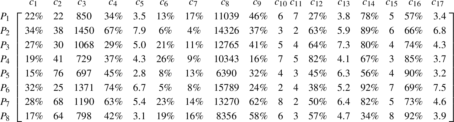

Step 2. We utilize Eqs. (1)–(3) to calculate three normalized decision matrices:

Integrate the above three normalized decision matrices by Eq. (4) to obtain a comprehensive decision matrix (here the two balance parameters are set as λ=0.4 and μ=0.3):

Step 3. Compute the average performance values of the providers on each criterion to form a virtual reference provider P0, which can be identified as (0.410, 0.395, 0.442, 0.381, 0.354, 0.369, 0.426, 0.366, 0.394, 0.398 0.316, 0.388, 0.417, 0.483, 0.382, 0.458, 0.340). Calculate the subordinate comprehensive values of the providers by Eqs. (5) and (6). Without loss of generality, we let the preference parameters δ=0.5 and ϑ=0.5. The results are displayed in Table 3.

Step 4. Calculate the final comprehensive values of providers by Eq. (7), and rank the providers according to the descending order of the final comprehensive values. The ranking results of the providers are listed in Table 3. We can determine that the optimal provider is P8.

5Sensitivity Analyses and Comparative Analyses

In this section, based on the data in Section 4, sensitivity analyses of the parameters set in the proposed method are carried out to explore the impact of the changes of parameters and criterion weights on the final ranking results of the alternatives. Moreover, other MCDM methods are applied to derive the ranking results of the alternatives, and the advantages of the proposed method are highlighted by comparing these results with that of the proposed method.

5.2Comparative Analyses

In this subsection, we compare the proposed method with various MCDM methods, including the TOPSIS, VIKOR, WASPAS, ARAS, and MULTIMOORA. The reason for comparison with the TOPSIS method is that both methods use the idea of reference points. The reason for comparison with the VIKOR method is that both methods use the linear max-min normalization. The reason for comparison with the WASPAS method is that both methods use the linear ratio-based normalization technique and the combination of arithmetic weighted aggregation operator and geometric weighted aggregation operator. The reason for comparison with the ARAS method is that both methods use the sum-based normalization technique and arithmetic weighted aggregation operator. The reason for comparison with the MULTIMOORA method is that both methods take into account the compensation and non-compensation effects among criteria.

5.2.1Comparative Analysis Between the Proposed Method and the TOPSIS Method

TOPSIS method, introduced by Hwang and Yoon in 1981, deduces the optimal alternative with the shortest distance from the positive ideal solution and the farthest distance from the negative ideal solution (Opricovic and Tzeng, 2004). The procedure of the TOPSIS method is as follows. First, normalize the decision matrix by the vector normalization technique (Eq. (8)). Second, determine two ideal solutions P+ and P− by Eqs. (9) and (10), respectively, and calculate the separation degrees of alternatives from two ideal solutions, Di+ and Di−, by Eqs. (11) and (12), respectively. Finally, calculate the relative closeness degrees of alternatives by Eq. (13) to attain the ranking of alternatives. The results obtained by the TOPSIS method based on the data in Section 4 are shown in Table 7.

(8)

x˜ij=xij∑i=1m(xij)2,

(9)

P+={(maxi(wjx˜ij)|j∈g),(mini(wjx˜ij)|j∈g′)|i=1,2,…,m}P+={x˜1+,x˜2+,…,x˜j+},

(10)

P−={(mini(wjx˜ij)|j∈g),(maxi(wjx˜ij)|j∈g′)|i=1,2,…,m}P−={x˜1−,x˜2−,…,x˜j−},

(11)

Di+=∑j=1n(wjx˜ij−x˜j+)2,i=1,2,…,m,

(12)

Di−=∑j=1n(wjx˜ij−x˜j−)2,i=1,2,…,m,

(13)

RCi=Di−/(Di−+Di+),i=1,2,…,m,

where x˜ij represents the normalized performance value of the ith alternative under the jth criterion. In Eqs. (9) and (10), g is associated with the benefit criteria while g′ is associated with the cost criteria.

Table 7

The results obtained by the TOPSIS method.

Providers	Di+	Di−	RCi	Ranks
P1	0.0439	0.0645	0.5951	2
P2	0.0686	0.0374	0.3526	8
P3	0.0451	0.0503	0.5274	5
P4	0.0476	0.0608	0.5609	4
P5	0.0574	0.0483	0.4571	6
P6	0.0704	0.0388	0.3550	7
P7	0.0449	0.0641	0.5877	3
P8	0.0376	0.0659	0.6368	1

Comparing the ranking result of the proposed MACONT method and that of the TOPSIS method, except for P2, P6 and P8, the ranks of other providers are different. Both methods set up a reference alternative to measure the distance between each alternative and the reference alternative. The main reason for the different results may be that the two methods adopt different normalization techniques, and the TOPSIS method needs to set up the best and worst reference alternatives to measure the distances between alternatives and the two reference alternatives, while the MACONT method only needs to set up one reference alternative to measure the good and bad performance of alternatives.

5.2.2Comparative Analysis Between the Proposed Method and the VIKOR Method

VIKOR method, proposed by Opricovic in 1998, aims to find a compromise solution between maximum “group utility” of the “majority” and minimum “individual regret” of the “opponent” (Opricovic and Tzeng, 2007). The VIKOR method firstly normalizes each element in the decision matrix by Eq. (14), and then computes the group utility value Ki and the individual regret value Ri by Eqs. (15) and (16), respectively. Next, the method calculates the compromise value Ci by Eq. (17). Finally, according to the ranks on Ki, Ri and Ci, three ranking lists are obtained. The results deduced by the VIKOR method based on the data in Section 4 are shown in Table 8.

(14)

xˆij∗=(maxixij−xij)/(maxixij−minixij),for benefit criteria,xˆij∗=(minixij−xij)/(minixij−maxixij),for cost criteria,

(15)

Ki=∑j=1n(wjxˆij∗),i=1,2,…,m,

(16)

Ri=maxj(wjxˆij∗),i=1,2,…,m,

(17)

Ci=αmaxKi−KimaxKi−minKi+(1−α)maxRi−RimaxRi−minRi,i=1,2,…,m,

where xˆij∗ represents the normalized performance value of the ith alternative under the jth criterion, and α is a parameter whose value is determined by experts according to their preferences. Without loss of generality, we set α=0.5.

Table 8

The results obtained by the VIKOR method.

Providers	Ki	Rank	Ri	Rank	Ci	Ranks
P1	0.4754	5	0.0800	6	0.4391	5
P2	0.6256	7	0.0980	7	0.8680	7
P3	0.4692	4	0.0590	2	0.2551	3
P4	0.4491	3	0.0720	4	0.3240	4
P5	0.5178	6	0.0753	5	0.4801	6
P6	0.6304	8	0.1130	8	1.0000	8
P7	0.4361	2	0.0637	3	0.2316	2
P8	0.3632	1	0.0521	1	0.0000	1

Comparing the ranking result deduced by the proposed MACONT method and that obtained by the VIKOR method, except for P7 and P8, the ranks of other providers are different. The reasons for this phenomenon may be as follows. In terms of normalization technique, the third normalization technique used in the MACONT method (Eq. (3)) is similar to the normalization technique used in the VIKOR method (Eq. (8)), but the larger the normalized value of an alternative in the proposed method is and the smaller the normalized value of an alternative is in the VIKOR method, the better the final rank of the alternative will be. Furthermore, the VIKOR method only uses one normalization technique, while the proposed method synthesizes three normalization techniques. In terms of aggregation operator, the VIKOR method applies the arithmetic weighted aggregation operator and considers the worst performance of alternatives over all criteria, while the MACONT method applies the combination of arithmetic weighted aggregation operator and arithmetic weighted aggregation operator; that is to say, the MACONT method considers the good and bad performance of alternatives on all criteria simultaneously.

5.2.3Comparative Analysis Between the Proposed Method and the WASPAS Method

WASPAS method, introduced by Zavadskas et al. (2012), firstly normalizes each element in the decision matrix by the linear ratio-based normalization technique (Eq. (2)), and then the normalized performance values of alternatives on all criteria are aggregated by the arithmetic weighted aggregation operator (Eq. (18)) and the geometric weighted aggregation operator (Eq. (19)). Afterwards, a parameter β (here β=0.5) is introduced to combine the values deduced by Eqs. (18) and (19). Finally, the comprehensive score of each alternative can be obtained by Eq. (20) to determine the ranking of alternatives. The results deduced by the WASPAS method based on the data in Section 4 are shown in Table 9.

(18)

Gi1=∑j=1n(wjxˆij2),i=1,2,…,m,

(19)

Gi2=∏j=1n(xˆij2)wj,i=1,2,…,m,

(20)

Gi=βGi1+(1−β)Gi2,i=1,2,…,m.

Table 9

The results obtained by the WASPAS method.

Providers	Gi1	Gi2	Gi	Ranks
P1	0.7028	0.6715	0.6871	3
P2	0.5764	0.5245	0.5504	8
P3	0.6750	0.6619	0.6685	4
P4	0.6844	0.6412	0.6628	5
P5	0.6477	0.6021	0.6249	6
P6	0.5844	0.5306	0.5575	7
P7	0.7155	0.6762	0.6958	2
P8	0.7437	0.7088	0.7262	1

Comparing the ranking result of the proposed MACONT method and that of the WASPAS method, the ranks of P1, P3, P4 and P5 are different. Although both methods use the linear ratio-based normalization technique and the combination of arithmetic weighted aggregation operator and geometric weighted aggregation operator, the WASPAS method only considers one kind of normalization technique and the aggregation operator is aimed at aggregating the performance values of alternatives, while the MACONT method synthesizes three kinds of normalization techniques and the aggregation operator is aimed at aggregating the distances between each alternative and the virtual reference alternative.

5.2.4Comparative Analysis Between the Proposed Method and the ARAS Method

ARAS method, presented by Zavadskas and Turskis (2010), firstly sets the optimal alternative P0′(x01,x02,…,x0n) as the reference alternative by Eq. (21), and then normalizes the decision matrix by the linear sum-based normalization technique (Eq. (1)). Next, the normalized performance values of alternatives on all criteria are aggregated by the arithmetic weighted aggregation operator (Eq. (22)). Afterwards, the utility degrees of alternatives can be calculated by Eq. (23) to determine the ranking of alternatives in descending order. The results deduced by the ARAS method based on the data in Section 4 are shown in Table 10.

(21)

x0j=maxixij,for benefit criteria,x0j=minixij,for cost criteria,j=1,2,…,n,

(22)

Zi=∑j=1n(wjxˆij1),i=0,1,2,…,m,

(23)

UDi=Zi/Z0,i=0,1,2,…,m.

Table 10

The results obtained by the ARAS method.

Providers	Zi	UDi	Ranks
P0′	0.1593	1.0000	–
P1	0.1123	0.7054	3
P2	0.0904	0.5678	8
P3	0.1066	0.6694	5
P4	0.1083	0.6798	4
P5	0.1012	0.6356	6
P6	0.0921	0.5781	7
P7	0.1126	0.7070	2
P8	0.1172	0.7358	1

Comparing the ranking result of the proposed MACONT method and that of the ARAS method, the ranks of P1, P3, P4 and P5 are different. Both methods use the linear sum-based normalization technique, but the MACONT method also integrates the other two normalization techniques. In terms of the aggregation methods, only the arithmetic weighted aggregation operator is used in the ARAS method, while the geometric weighted average operator is also used in the MACONT method. Furthermore, in the setting of the reference alternative, the ARAS method sets the best performance of alternatives on all criteria as the reference alternative and determines the alternative ranking according to the ratio of utility degrees of alternatives and the reference alternative, while the MACONT method sets the average performance of alternatives on all criteria as the reference alternative and determines the alternative ranking based on the distance between each alternative and the reference alternative.

5.2.5Comparative Analysis Between the Proposed Method and the MULTIMOORA Method

MULTIMOORA method, proposed by Brauers and Zavadskas (2010), exploits three subordinate ranking methods to obtain three ranking lists based on the decision matrix which is normalized by the vector normalization technique (Eq. (8)). The first subordinate ranking method is the Ratio System, and the utility values of alternatives can be calculated by Eq. (24). The second subordinate ranking method is the Reference Point Approach, and the utility values of alternatives can be calculated by Eq. (25). The third subordinate ranking method is the Full Multiplicative Form, and the utility values of alternatives can be calculated by Eq. (26). Afterwards, this method aggregates the three subordinate ranking results based on the dominance theory (Brauers and Zavadskas, 2011) to determine the final ranking of alternatives. The results derived by the MULTIMOORA method based on the data in Section 4 are shown in Table 11.

(24)

Yi1=∑j=1g(wjx˜ij)−∑j=1g′(wjx˜ij),i=1,2,…,m,

(25)

Yi2=maxj[wj(maxix˜ij−x˜ij)],for benefit criteria,Yi2=maxj[wj(x˜ij−minix˜ij)],for cost criteria,i=1,2,…,m,

(26)

Yi3=∏j=1g(x˜ij)wj/∏j=1g′(x˜ij)wj,i=1,2,…,m.

Table 11

The results obtained by the MULTIMOORA method.

Providers	Yi1	Ranks	Yi2	Ranks	Yi3	Ranks	Final ranks
P1	0.1973	3	0.0276	5	0.5883	3	4
P2	0.1309	7	0.0369	7	0.4595	8	7
P3	0.1853	5	0.0219	1	0.5799	4	3
P4	0.1909	4	0.0232	3	0.5617	5	5
P5	0.1524	6	0.0292	6	0.5275	6	6
P6	0.1303	8	0.0439	8	0.4648	7	8
P7	0.1999	2	0.0251	4	0.5924	2	2
P8	0.2150	1	0.0229	2	0.6210	1	1

Comparing the ranking result of the proposed MACONT method and that of the MULTIMOORA method, we can find that the ranks of other providers are different except for P1, P7 and P8. Although the two methods are similar in the form of aggregation method, and both of them take into account the compensation and non-compensation effects among criteria, the two methods are quite different. On the one hand, the MULTIMOORA method only uses the vector normalization technique, while the MACONT method comprehensively uses three linear normalization techniques. On the other hand, the MULTIMOORA method divides the criteria into different types in the process of aggregation. It is easy to see that the MULTIMOORA method can only be applied to solve the MCDM problems with both cost and benefit criteria, while the MACONT method first divides the criteria types in the process of normalization, which reduces the amount of calculation to a certain extent and has a wider scope of application than the MULTIMOORA method.

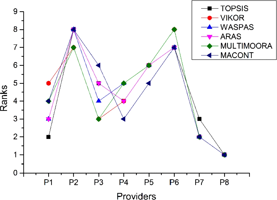
The ranks of providers obtained by the proposed MACONT method and the aforementioned methods are displayed in Fig. 1. From this figure, we can find that the ranking results derived by each MCDM method are different, and the ranks result of the providers derived by the proposed MACONT method is a comprehensive solution.

Fig. 1

Comparison of the MACONT method and the other MCDM methods.

6Conclusion

This study mainly proposed an MACONT method which involves a comprehensive normalization technique based on criterion types and two mixed aggregation operators to aggregate the distance values between each alternative and the reference alternative on different criteria from the perspectives of compensation and non-compensation. To testify the applicability of the proposed method, an illustration example regarding the selection of sustainable third-party reverse logistics providers was given. Through the sensitivity analyses and comparative analyses, we highlight that the proposed MACONT method has the following advantages:

In this study, there is a deficiency that we did not analyse the impact of the change of criterion weights on the final result derived by the proposed method, because the number of criteria in the illustration example is large, and it is not easy to grasp the influence of the change of criterion weights on the ranking results. In the future, we will analyse this problem. In addition, we will consider to combine the proposed method with the fuzzy set theory, extending the proposed method to intuitionistic fuzzy environment, hesitant fuzzy linguistic environment and probabilistic linguistic environment to solve complex decision-making problems in various fields.

References

1 | Aggarwal, M. ((2017) ). Discriminative aggregation operators for multi criteria decision making. Applied Soft Computing, 52: , 1058–1069. https://doi.org/10.1016/j.asoc.2016.09.025. |
2 | Alinezhad, A., Khalili, J. ((2019) ). New Methods and Applications in Multiple Attribute Decision Making (MADM). International Series in Operations Research & Management Science, Vol. 277: . Springer, Switzerland. https://doi.org/10.1007/978-3-030-15009-9. |
3 | Bai, C., Sarkis, J. ((2019) ). Integrating and extending data and decision tools for sustainable third-party reverse logistics provider selection. Computers & Operations Research, 110: , 188–207. https://doi.org/10.1016/j.cor.2018.06.005. |
4 | Bana e Costa, C.A., Chagas, M.P. ((2004) ). A career choice problem: an example of how to use MACBETH to build a quantitative value model based on qualitative value judgments. European Journal of Operational Research, 153: (2), 323–331. https://doi.org/10.1016/s0377-2217(03)00155-3. |
5 | Blanco-Mesa, F., León-Castro, E., Merigó, J.M. ((2019) ). A bibliometric analysis of aggregation operators. Applied Soft Computing, 81: , 105488. https://doi.org/10.1016/j.asoc.2019.105488. |
6 | Brauers, W.K.M., Zavadskas, E.K. ((2009) ). Robustness of the multi-objective MOORA method with a test for the facilities sector. Technological and Economic Development of Economy, 15: (2), 352–375. https://doi.org/10.3846/1392-8619.2009.15.352-375. |
7 | Brauers, W.K.M., Zavadskas, E.K. ((2010) ). Project management by MULTIMOORA as an instrument for transition economies. Technological and Economic Development of Economy, 16: (1), 5–24. https://doi.org/10.3846/tede.2010.01. |
8 | Brauers, W.K.M., Zavadskas, E.K. ((2011) ). MULTIMOORA optimization used to decide on a bank loan to buy property. Technological and Economic Development of Economy, 17: (1), 174–188. https://doi.org/10.3846/13928619.2011.560632. |
9 | Chen, P. ((2019) ). Effects of normalization on the entropy-based TOPSIS method. Expert Systems with Applications, 136: , 33–41. https://doi.org/10.1016/j.eswa.2019.06.035. |
10 | Diakoulaki, D., Mavrotas, G., Papayannakis, L. ((1995) ). Determining objective weights in multiple criteria problems: the CRITIC method. Computers & Operations Research, 22: (7), 763–770. https://doi.org/10.1016/0305-0548(94)00059-h. |
11 | Emovon, I., Norman, R.A., Murphy, A.J. ((2016) ). Methodology of using an integrated averaging technique and MAUT method for failure mode and effects analysis. Journal of Engineering and Technology, 7: (1), 140–155. http://journal.utem.edu.my/index.php/jet/article/view/777. |
12 | Gomes, L.F.A.M. ((2009) ). An application of the TODIM method to the multicriteria rental evaluation of residential properties. European Journal of Operational Research, 193(1): , 204–211. https://doi.org/10.1016/j.ejor.2007.10.046. |
13 | Govindan, K., Jepsen, M.B. ((2016) ). ELECTRE: a comprehensive literature review on methodologies and applications. European Journal of Operational Research, 250: (1), 1–29. https://doi.org/10.1016/j.ejor.2015.07.019. |
14 | Govindan, K., Kadziński, M., Ehling, R., Miebs, G. ((2018) ). Selection of a sustainable third-party reverse logistics provider based on the robustness analysis of an outranking graph kernel conducted with ELECTRE I and SMAA. Omega, 85: , 1–15. https://doi.org/10.1016/j.omega.2018.05.007. |
15 | Hwang, C.L., Yoon, K. ((1981) ). Multiple Attribute Decision Making-Methods and Applications: A State-of-the-Art Survey. Lecture Notes in Economics and Mathematical Systems, Vol. 186: . Springer-Verlag, Berlin, Heidelberg. https://doi.org/10.1007/978-3-642-48318-9. |
16 | Jahan, A., Edwards, K.L. ((2015) ). A state-of-the-art survey on the influence of normalization techniques in ranking: improving the materials selection process in engineering design. Materials & Design, (1980–2015), 65: , 335–342. https://doi.org/10.1016/j.matdes.2014.09.022. |
17 | Jharkharia, S., Shankar, R. ((2007) ). Selection of logistics service provider: an analytic network process (ANP) approach. Omega, 35: (3), 274–289. https://doi.org/10.1016/j.omega.2005.06.005. |
18 | Keshavarz Ghorabaee, M., Zavadskas, E.K., Olfat, L., Turskis, Z. ((2015) ). Multi-criteria inventory classification using a new method of evaluation based on distance from average solution (EDAS). Informatica, 26: , 435–451. https://doi.org/10.15388/Informatica.2015.57. |
19 | Kou, G., Lu, Y., Peng, Y., Shi, Y. ((2012) ). Evaluation of classification algorithms using MCDM and rank correlation. International Journal of Information Technology & Decision Making, 11: (01), 197–225. https://doi.org/10.1142/s0219622012500095. |
20 | Kou, G., Yang, P., Peng, Y., Xiao, F., Chen, Y., Alsaadi, F.E. ((2020) ). Evaluation of feature selection methods for text classification with small datasets using multiple criteria decision-making methods. Applied Soft Computing, 86: , 105836. https://doi.org/10.1016/j.asoc.2019.105836. |
21 | Krylovas, A., Zavadskas, E.K., Kosareva, N., Dadelo, S. ((2014) ). New KEMIRA method for determining criteria priority and weights in solving MCDM problem. International Journal of Information Technology & Decision Making, 13: (06), 1119–1133. https://doi.org/10.1142/s0219622014500825. |
22 | Lahtinen, T.J., Hämäläinen, R.P., Jenytin, C. ((2020) ). On preference elicitation processes which mitigate the accumulation of biases in multi-criteria decision analysis. European Journal of Operational Research, 282: (1), 201–210. https://doi.org/10.1016/j.ejor.2019.09.004. |
23 | Liao, H.C., Wu, X.L. ((2020) ). DNMA: a double normalization-based multiple aggregation method for multi-expert multi-criteria decision making. Omega, 94: , 102058. https://doi.org/10.1016/j.omega.2019.04.001. |
24 | Liao, H.C., Xu, Z.S., Herrera-Viedma, E., Herrera, F. ((2018) ). Hesitant fuzzy linguistic term set and its application in decision making: a state-of-the art survey. International Journal of Fuzzy Systems, 20: (7), 2084–2110. https://doi.org/10.1007/s40815-017-0432-9. |
25 | Liao, H.C., Wen, Z., Liu, L.L. ((2019) ). Integrating BWM and ARAS under hesitant linguistic environment for digital supply chain finance supplier section. Technological and Economic Development of Economy, 25: (6), 1188–1212. https://doi.org/10.3846/tede.2019.10716. |
26 | Liao, H.C., Mi, X.M., Xu, Z.S. ((2020) ). A survey of decision-making methods with probabilistic linguistic information: bibliometrics, preliminaries, methodologies, applications and future directions. Fuzzy Optimization and Decision Making, 19: (1), 81–134. https://doi.org/10.1007/s10700-019-09309-5. |
27 | Mi, X.M., Liao, H.C., Wu, X.L., Xu, Z.S. ((2020) ). Probabilistic linguistic information fusion: a survey on aggregation operators in terms of principles, definitions, classifications, applications and challenges. International Journal of Intelligent Systems, 35: (3), 529–556. https://doi.org/10.1002/int.22216. |
28 | Opricovic, S., Tzeng, G.H. ((2004) ). Compromise solution by MCDM methods: a comparative analysis of VIKOR and TOPSIS. European Journal of Operational Research, 156: (2), 445–455. https://doi.org/10.1016/S0377-2217(03)00020-1. |
29 | Opricovic, S., Tzeng, G.H. ((2007) ). Extended VIKOR method in comparison with outranking methods. European Journal of Operational Research, 178: (2), 514–529. https://doi.org/10.1016/j.ejor.2006.01.020. |
30 | Pamucar, D., Cirovic, G. ((2015) ). The selection of transport and handling resources in logistics centers using multi-attributive border approximation area comparison (MABAC). Expert Systems with Applications, 42: (6), 3016–3028. https://doi.org/10.1016/j.eswa.2014.11.057. |
31 | Roy, B. ((1991) ). The outranking approach and the foundations of ELECTRE methods. Theory and Decision, 31: (1), 49–73. https://doi.org/10.1007/bf00134132. |
32 | Wu, X.L., Liao, H.C. ((2019) ). A consensus-based probabilistic linguistic gained and lost dominance score method. European Journal of Operational Research, 272: (3), 1017–1027. https://doi.org/10.1016/j.ejor.2018.07.044. |
33 | Yazdani, M., Zarate, P., Zavadskas, E.K., Turskis, Z. ((2019) ). A combined compromise solution (CoCoSo) method for multi-criteria decision-making problems. Management Decision, 57: (9), 2501–2519. https://doi.org/10.1108/MD-05-2017-0458. |
34 | Zarbakhshnia, N., Soleimani, H., Ghaderi, H. ((2018) ). Sustainable third-party reverse logistics provider evaluation and selection using fuzzy SWARA and developed fuzzy COPRAS in the presence of risk criteria. Applied Soft Computing, 65: , 307–319. https://doi.org/10.1016/j.asoc.2018.01.023. |
35 | Zarbakhshnia, N., Wu, Y., Govindan, K., Soleimani, H. ((2019) ). A novel hybrid multiple attribute decision-making approach for outsourcing sustainable reverse logistics. Journal of Cleaner Production, 242: , 118461. https://doi.org/10.1016/j.jclepro.2019.118461. |
36 | Zavadskas, E.K., Turskis, Z. ((2010) ). A new additive ratio assessment (ARAS) method in multicriteria decision-making. Technological and Economic Development of Economy, 16: , 159–172. https://doi.org/10.3846/tede.2010.10. |
37 | Zavadskas, E.K., Podvezko, V. ((2016) ). Integrated determination of objective criteria weights in MCDM. International Journal of Information Technology & Decision Making, 15: (02), 267–283. https://doi.org/10.1142/s0219622016500036. |
38 | Zavadskas, E.K., Turskis, Z., Antucheviciene, J., Zakarevicius, A. ((2012) ). Optimization of weighted aggregated sum product assessment. Elektronika ir elektrotechnika, 122: (6), 3–6. https://doi.org/10.5755/j01.eee.122.6.1810. |
39 | Zavadskas, E.K., Turskis, Z., Kildienė, S. ((2014) ). State of art surveys of overviews on MCDM/MADM methods. Technological and Economic Development of Economy, 20: (1), 165–179. https://doi.org/10.3846/20294913.2014.892037. |
40 | Zhang, H., Kou, G., Peng, Y. ((2019) ). Soft consensus cost models for group decision making and economic interpretations. European Journal of Operational Research, 277: , 964–980. https://doi.org/10.1016/j.ejor.2019.03.009. |
41 | Zolfani, S.H., Bahrami, M. ((2014) ). Investment prioritizing in high tech industries based on SWARA-COPRAS approach. Technological and Economic Development of Economy, 20: (3), 534–533. https://doi.org/10.3846/20294913.2014.881435. |