
An Effective Approach to Outlier Detection Based on Centrality and Centre-Proximity
Abstract
In data mining research, outliers usually represent extreme values that deviate from other observations on data. The significant issue of existing outlier detection methods is that they only consider the object itself not taking its neighbouring objects into account to extract location features. In this paper, we propose an innovative approach to this issue. First, we propose the notions of centrality and centre-proximity for determining the degree of outlierness considering the distribution of all objects. We also propose a novel graph-based algorithm for outlier detection based on the notions. The algorithm solves the problems of existing methods, i.e. the problems of local density, micro-cluster, and fringe objects. We performed extensive experiments in order to confirm the effectiveness and efficiency of our proposed method. The obtained experimental results showed that the proposed method uncovers outliers successfully, and outperforms previous outlier detection methods.
1Introduction
In contemporary research in different data-mining applications, outlier detection is a primary activity. Generally speaking, outliers represent extreme values that deviate from other observations on data. Often outliers are considered as a noise or an experimental error, however, they may bring some important information. Detected outliers usually are seen as potential candidates for abnormal data that may lead to model misspecification and incorrect results. However, in some situations, they can be considered as a novelty within the datasets. In other words, an outlier is an observation that diverges from an overall pattern on a sample. Two kinds of outliers can be distinguished: univariate and multivariate. Univariate outliers are connected to a distribution of values in a single feature space while multivariate outliers are connected to an n-dimensional space (of n-features). Outliers also can be classified as parametric or non-parametric as we consider a distribution of values for selected features.
In literature, there is no exact definition of an outlier as it highly depends on unseen assumptions about the data structure and the selected detection method. In our research, we concentrate on outliers as objects that are dissimilar to the majority of other objects (Barnett and Lewis, 1994; Han and Kamber, 2000; Hawkins, 1980; Akoglu et al., 2010; Huang et al., 2016; Yerlikaya-Ö et al., 2016; Domingues et al., 2018; Kieu et al., 2018). Detection of such outliers is of high importance for different applications and it is particularly based on specific datasets. Typical application domains include detecting misuse of medicines, detecting network intrusions (Song et al., 2013; Fanaee-T and Gama, 2016), and detecting economic and financial frauds (Chan et al., 2010; Friedman et al., 2007).
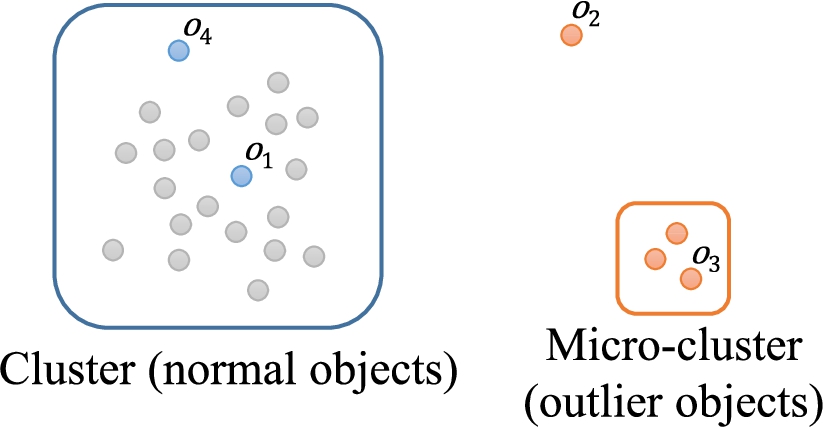
To illustrate our approach and understanding of outliers in this paper we will illustrate it visually. In Fig. 1, a 2-dimensional dataset is shown. There are many objects with characteristics similar to those of object
Fig. 1
A 2-dimensional dataset.
As nowadays outlier detection is a challenging research area, a wide range of methods is used (Bay and Schwabacher, 2003; Böhm et al., 2009; Breunig et al., 2000; Knorr and Ng, 1999; Knorr et al., 2000; Moonesinghe and Tan, 2008; Papadimitriou et al., 2003; Ramaswamy et al., 2000). The majority of these methods use their own object location features which reflect the relative characteristics of each object over the distribution of all objects in the dataset. The standard flow of activities is presented below:
• Step 1. Within the methods, the first activity is to compute location features of each object in the dataset.
• Step 2. After that, an outlierness score is assigned to the object that reflect those location features. In fact, an outlierness score of an object i indicates how much a different object i is compared to other objects in the dataset.
• Step 3. Finally, the methods consider as outliers the top m objects with the highest outlierness score.
The significant issue of existing outlier detection methods is that they extract location features only taking into account the characteristics of the object itself. They do not pay attention to the characteristics of its neighbouring objects nor the distribution of all of the objects in the dataset. Therefore, the location features of each object are highly dependent on the parameters given by users. This is the main reason for the well-known local density and micro-cluster problems (Papadimitriou et al., 2003). The key issue of these methods is that they are highly based on the location features of objects. Consequently, the local density problem is a phenomenon that outliers are determined only depending on its local density. The essential problem is the micro-cluster problem as in such circumstances micro-clusters cannot be detected as outliers.
Additional quality of some methods is that when calculating the outlierness score of each object, they consider not only the location features of the object itself but also the location features of its neighbouring objects (Breunig et al., 2000). However, because of the fundamental limitations of their location features that do not consider the distributions of all objects in the dataset, they still have the micro-cluster problem.
Having in mind the above mentioned limitations of existing methods, in this paper we are going to propose a novel approach.11 First, we propose the notions of centrality and centre-proximity as novel relative location features that can take into consideration the characteristics of all the objects in the dataset, rather than only the characteristics of the object itself. Furthermore, we propose a graph-based method for outlier detection that calculates the outlierness score of each object using these two newly introduced relative location features. Our method models a given dataset as a k-NN graph and calculates the centrality and centre-proximity scores of each object from the k-NN graph iteratively. To show the effectiveness of our method, we carried out a variety of experiments. The obtained results are promising and also compared with the previous outlier detection methods, our method achieves the best precision.
The rest of the paper is organized as follows. Section 2 is devoted to some existing outlier detection methods and points out their deficiencies. Section 3 brings an overview of our proposed method and outlines its main four goals. Technical details of our method are presented in Section 4. In Section 5, we explain graph modelling schemes for our graph-based outlier detection. Experimental results of performance analysis to verify the superiority of our method are presented in Section 6. Finally, Section 7 brings concluding remarks and possibilities for future work.
2Related Work
In this section, we first introduce previous outlier detection methods, which are statistics-based, distance-based, density-based, and RWR-based methods. We then point out their problems in outlier detection.
2.1Statistics-Based Outlier Detection
The statistics-based outlier detection method finds the most suitable statistical distribution model for the distribution of objects in the given dataset and detects the objects that deviate from the statistical distribution model as outliers (Chandola et al., 2009).
If the dataset is generated under a specific statistical distribution model, the statistics-based outlier detection method will work well as a feasible solution to the detection of outliers. However, the problem is that most real-world data is not generated from a specific statistical distribution model (Chandola et al., 2009; Knorr and Ng, 1999; Knorr et al., 2000). Additionally, when detecting outliers from a multi-dimensional dataset, it is very difficult to find a statistical distribution model that can fit the distribution of almost all objects in the dataset in terms of all dimensions (Chandola et al., 2009; Knorr and Ng, 1999; Knorr et al., 2000).
2.2Distance-Based Outlier Detection
The distance-based outlier detection method uses the distance among objects as a location feature, and detects as outliers the ones whose distance to other objects exceed a specific threshold (Ramaswamy et al., 2000). Here, the threshold is a user-defined parameter.
There have been several previous studies on distance-based outlier detection. The DB-outlier method (Knorr and Ng, 1999; Knorr et al., 2000) uses the number of other objects near the target object o to find out whether o is an outlier or not. If there are less than p objects within the distance d from o, o is considered an outlier. k-Dist method (Ramaswamy et al., 2000) uses the k-Dist as a location feature, and detects the top m objects having the largest k-Dist value as outliers. Here, the k-Dist is the distance from each object to its k-th nearest object.
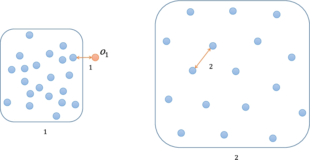
Distance-based outlier detection methods use the features that only consider the characteristics of the object itself. Thus, it could cause the local density problem (Papadimitriou et al., 2003). Figure 2 shows an example of a 2-dimensional dataset with the local density problem. The dataset has two clusters (
Fig. 2
An example of the local density problem.
2.3Density-Based Outlier Detection
The density-based outlier detection methods classify an object as an outlier by considering the relative density of the target object (Breunig et al., 2000). The density of an object could be decided by the number of objects around it.
The LOF method (Breunig et al., 2000; Na et al., 2018) is a typical example of the density-based outlier detection. The LOF method defines the density of an object as the average reachability distance from the object to its k-nearest objects. Here, the reachability distance from object p to object q is a large value between the distance of the two objects and the distance between q and the k-th nearest object of q. In the LOF method, an object p has a high outlierness score if the density of p is lower than that of p’s neighbouring objects.
Fig. 3
An example of the micro-cluster problem.
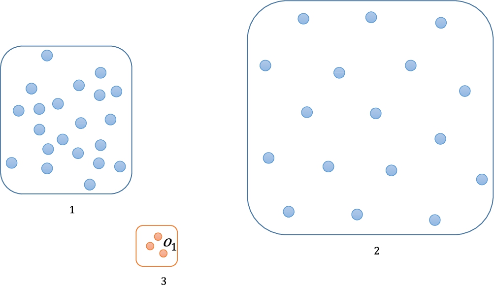
The density-based methods consider the characteristics of the target object itself by comparing it with its neighbouring objects. By considering neighbouring objects altogether, the local density problem is prevented. However, in density-based methods there still exists the micro-cluster problem (Moonesinghe and Tan, 2008).
Figure 3 shows an example of a 2-dimensional dataset with the micro-cluster problem. The dataset includes two clusters (
This problem arises because they take only the neighbouring objects into account when determining if an object is an outlier. Thus, we should also consider the characteristics of all the objects in the dataset to overcome the micro-cluster problem and the local-density problem.
2.4RWR-Based Outlier Detection
The RWR-based outlier detection methods (Moonesinghe and Tan, 2008) model a given dataset as a graph, and perform the Random Walk with Restart (RWR) (Brin and Page, 1998) on the modelled graph to detect outliers. Here, the inversed number of the RWR score of each object is considered as its outlierness score.
There are two methods in RWR-based outlier detections. The Outrank-a method models a given dataset as a complete weighted graph where weights are the similarity between every pair of objects and the Outrank-b method, from the same complete weighted graph, deletes the edges with the similarity lower than a specific threshold t. Because these methods use a graph, they have the advantage that the characteristics of all the objects could be considered when deciding whether or not an object is an outlier.
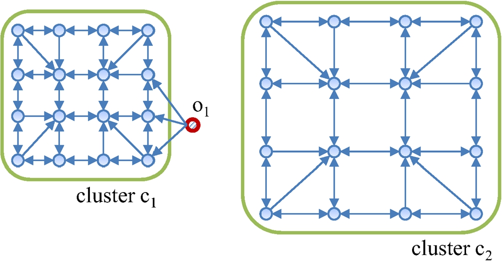
However, in the RWR-based methods, the RWR score is transferred through a directed edge in a single direction, and they cannot differentiate the fringe objects from the outlier objects. Furthermore, the Outrank-a method, which models a dataset as a complete graph, directly considers the characteristics of all the other objects. As a result, the precision of outlier detection is low. In the case of Outrank-b, the precision of outlier detection is greatly affected by the user-defined parameter value t. These problems will be discussed in Sections 4 and 5 in more detail.
3Overview
In this section, we define our goals of outlier detection and explain our strategies to achieve the goals. The following is our list of goals in detecting outliers.
• Goal 1: Outliers should be accurately detected. The proposed method should avoid the local density problem and the micro-cluster problem. Furthermore, the fringe objects in clusters should not be classified as outliers.
• Goal 2: For every object in a dataset, the proposed method should not only determine if it is an outlier or not, but also provide an outlierness score of each object to the user. The user can use this score to understand how much an object deviates from normal objects and can decide the number of outliers intuitively. Moreover, the user also can observe the changes in the outlierness score of each object occurred by the change in the user-defined parameter values. This provides the user with hints on setting the parameter values.
• Goal 3: The proposed method should be able to handle data of any type and/or any form. The proposed method should be applicable to multi-dimensional data, non-coordinate data, and more, in contrast to the statistics-based outlier detection method that has limitations on the applicable data form.
• Goal 4: The number of user-defined parameters should be as small as possible, and the fluctuation of the precision by the change in user-defined parameter values should be small. In general circumstances, the user would not have a perfect understanding on a given dataset. Thus, our proposed method should not be sensitive to its parameters and provide reasonable accuracy with non-optimal parameters.
We propose a novel outlier detection method to achieve the goals above. First, we propose two novel location features called centrality and centre-proximity. Both features could make our proposed method avoid the local-density problem and the micro-cluster problem by taking the characteristics of each object, its neighbouring objects, and all the objects in the dataset into account (Goal 1). Centrality and centre-proximity also provide robustness on parameters to our proposed method (Goal 4).
Fig. 4
Overview of the proposed method (
Second, we build a k-NN graph from a given dataset and analyse the modelled graph to compute the outlierness score for each object. Thus, our method provides users with an outlierness score of every object (Goal 2). It is noteworthy that multidimensional data and/or non-coordinate data can also be modelled as a graph. Therefore, by using such a strategy, we can relax the constraints on the input data types and/or forms (Goal 3).
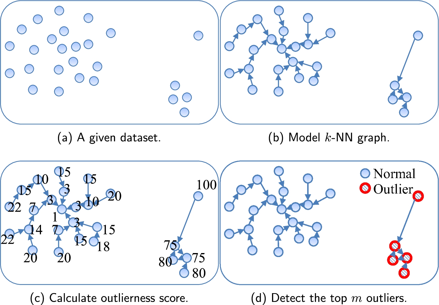
As shown in Fig. 4, the proposed method has three steps to detect outliers.
1. Build a k-NN graph from a given dataset. Each object in the dataset is represented as a node, the k-NN relationships connecting each object to its k-nearest objects are represented as directed edges. Each edge has the weight value of the similarity between the two nodes it connects.
2. For each object in the dataset, calculate the centrality and centre-proximity scores on the k-NN graph. Using both scores, compute the outlierness score of each node.
3. Return the top m objects with the highest outlierness scores as outliers.
4Centrality and Centre-Proximity
An object near the centre of a cluster is more likely to have many neighbouring objects than outliers. The distances between such an object and its neighbouring objects would be closer than the distances between an outlier object and its neighbouring objects. We propose two novel location features representing above properties that differentiate the normal objects and the outlier objects: the centrality and centre-proximity.
To calculate centrality and centre-proximity, we convert the given dataset into a graph as in existing RWR-based outlier detection methods. Although there are different ways to build a graph out of a given dataset, we use the k-NN graph for the conversion. We discuss different graph modelling schemes in Section 5.
Centrality represents how much other objects in the dataset recognize a target object p as one of the core objects within the cluster. Centre-proximity represents how close a target object p is to the core objects within the cluster.
The centrality score can be measured by how many other objects recognize the target object p as their neighbour. The influence of each object that recognizes p as its neighbour is proportional to its centre-proximity and how much close it is to p. On the other hand, the centre-proximity score can be measured by how many other objects are recognized by p as its neighbour. The influence of each object recognized by p as its neighbour is also proportional to its centrality and how much close it is to p.
We compute the two scores by iteratively referring to each other. The centrality and centre-proximity of node p can be calculated in the i-th iteration as follows:
(1)
(2)
As the two equations above show, centrality and centre-proximity scores have a mutual reinforcement relationship with each other. A high centreality object makes the centre-proximity scores of the objects regarding it as their neighbour increase. Respectively, a high centre-proximity object makes the centrality scores of the objects regarded as its neighbour increase. This mutual reinforcement relationship between the centrality and centre-proximity scores is similar to that between the hub and authority scores in HITS (Kleinberg, 1999).
Second, the centrality and centre-proximity scores of an object have the influence on its neighbouring objects in proportion to the weights on the edges. This means that an object has a larger influence on an object close to itself than a far apart object. This concept is unique with our approach and is not reflected in the mutual reinforcement of HITS.
The detailed procedure for calculating the two scores is shown in Fig. 5. The number of iterations (MAX_ITERATIONS) decides how far an object influences other objects in calculating the centrality and centre-proximity scores. If the influence of only directly connected neighbours is to be considered, we set MAX_ITERATIONS as 1. On the other hand, if the influence of all the objects in the dataset needs to be considered, we set MAX_ITERATIONS as the diameter of the modelled graph (Ha et al., 2011).
Fig. 5
Procedure of calculating the outlierness scores.
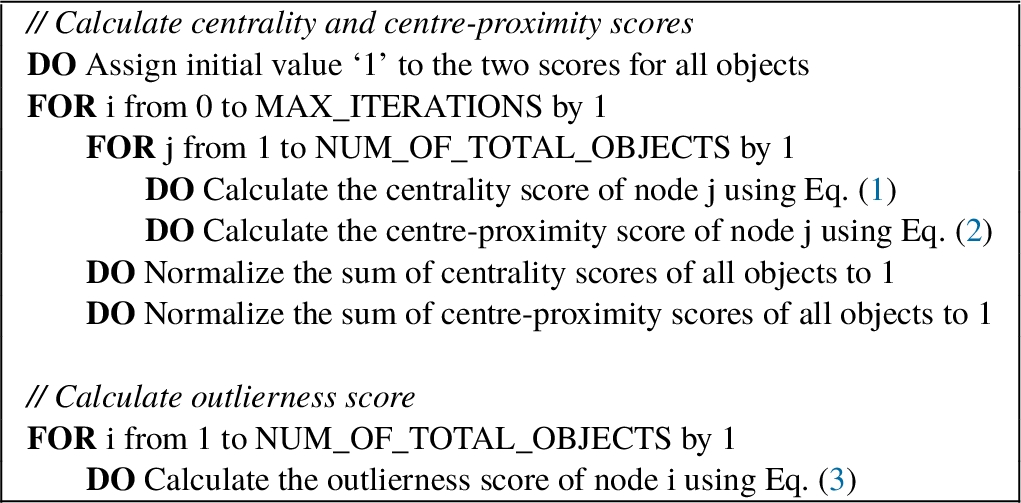
By iteratively calculating the centrality and centre-proximity scores, each object gets the centrality and centre-proximity scores that are affected by its indirect neighbours. With sufficiently large MAX_ITERATIONS (i.e. MAX_ITERATIONS equal to or greater than the diameter of the graph), both scores are affected by all the objects in the dataset. This makes the proposed outlier detection method prevent both local density and micro-cluster problems.
The outliers get low centrality and centre-proximity scores compared to those of the normal objects. The fringe objects may have low centrality scores as the outliers but their centre-proximity scores would be generally higher than that of the outliers. To fulfill Goal 1, we use the inverse of the converged centre-proximity score of each object as the final outlierness score. The outlierness score of node p can be calculated as follows:
(3)
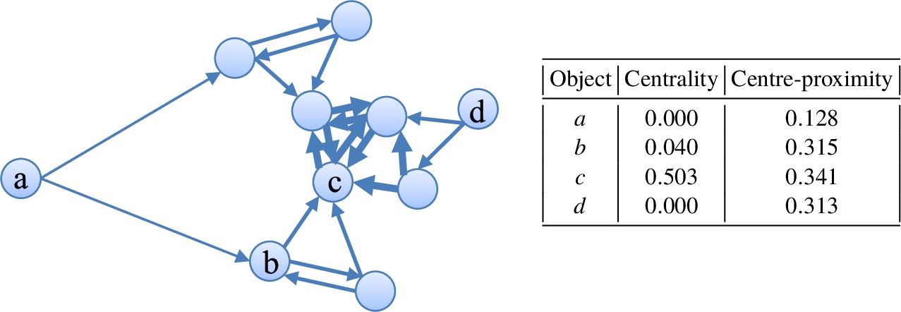
Figure 6 shows the centrality and centre-proximity scores assigned to each object on a 2-NN graph where edge
Fig. 6
Centrality and centre-proximity scores assigned to objects in a 2-NN graph.
The RWR score, the location feature in the RWR-based outlier detection method, considers (1) how many objects point to an object, and (2) how many objects exist around the object. Therefore, the RWR score is similar in concepts to the centrality score, and thus it cannot differentiate the fringe objects and the outlier objects.
The proposed method has an
5Graph Modelling
We model a graph based on the given dataset to easily calculate the centrality and centre-proximity scores. The neighbour relationship between two objects can be represented as an edge in the graph. In Section 5.1, we introduce the three graph modelling schemes to model a given dataset, and then analyse the effect of each scheme on our outlier detection method.
The centrality and centre-proximity scores of an object have influence on its neighbouring objects in proportion to the weights on the edges. The weight should have a high score if two objects have similar characteristics (i.e. located close to each other) and should have a low score if two objects are different (i.e. located far apart). The details of the weight assignment methods are discussed in Section 5.2.
5.1Graph Models
In this section, we analyse three graph modelling schemes, (1) a complete graph, (2) an e-NN graph, and (3) a k-NN graph, for our proposed outlier detection. The three graph modelling schemes are the same in representing an object as a node, and are different only in the way they connect nodes with edges. Note that we can model a given dataset as different graph modelling schemes such as minimum spanning tree graphs, k-NN graph variations, and e-k-NN graphs. However, we employ the three representative (base-formed) graph modelling schemes having quite different characteristics with each other.
5.1.1Complete Graph
A complete graph connects each node in the dataset to every other node with a directed edge. Due to this, the centrality and centre-proximity scores of an object are directly affected by all the other objects in the graph.
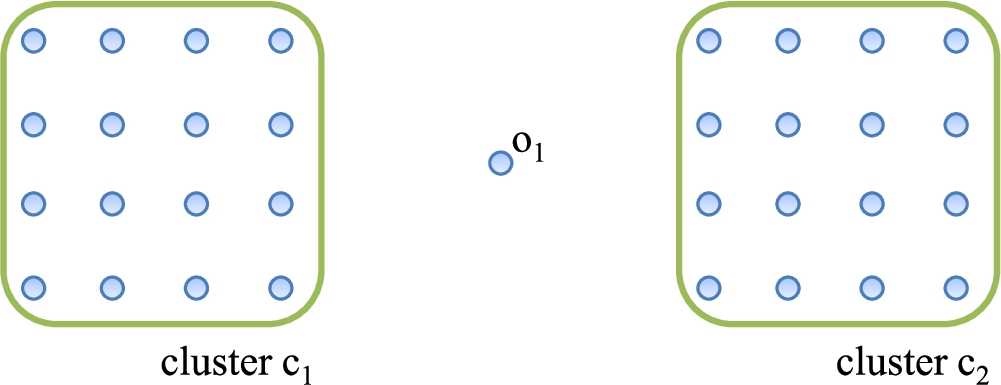
In the complete graph, the centrality and centre-proximity scores of each object show a difference only according to the weight values. Especially, the weights of the edges connected to objects located at the centre of gravity in the whole graph have the largest values. Therefore, the objects located at the centre of gravity have the highest centrality and centre-proximity scores with no relationship to whether they are outliers or not. Figure 7 shows a 2-dimensional dataset. The dataset includes two clusters (
Fig. 7
An example showing the problem with a complete graph.
Additionally, in the complete graph, the number of edges is the square of the total number of objects in the dataset, and therefore the performance of computing the centrality and center-proximity scores could deteriorate significantly.
5.1.2e-NN Graph
An e-NN graph modelling scheme connects an object with other objects that exist within a specific distance denoted as e as shown in Fig. 8. Due to this, the e-NN graphs for the same dataset could differ greatly when the value of e changes. In Fig. 8, if e is set to a value smaller than
Fig. 8
An example of the local density problem with an e-NN graph.
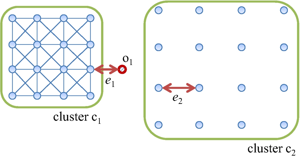
As a result, in the e-NN graph, the precision of the outlier detection changes considerably when e changes. Therefore, the user should understand the distribution of the dataset very well in order to set the proper value for e, which is quite difficult in practice.
5.1.3k-NN Graph
A k-NN graph modelling scheme connects each object to its k nearest objects with a directed edge as shown in Fig. 9. Therefore, in the k-NN graph, each object directly affects its nearest k objects.
Fig. 9
An example of a distinguishable outlier problem with a directed k-NN graph (
In the k-NN graph, the out-degrees of all objects are identical but the in-degrees of objects vary depending on how many other objects regard it as its k-NN. The objects near the core of the cluster have high in-degrees, and thus have high centrality and centre-proximity scores. The outliers and the fringe objects have small in-degrees, and thus have low centrality scores. However, the fringe objects have more out-edges that are pointing to high centre-proximity objects than the outlier objects, and thus show higher centre-proximity scores than those of the outliers. Therefore, it is possible to differentiate outliers and fringe objects with the k-NN graph.
The precision of outlier detection using the k-NN graph may change with the change in a parameter value of k. When k is very small, objects are sparsely connected and may not be able to clearly form a cluster. As a result, the precision of detecting outliers decreases. As k increases, the clusters are clearly formed, and thus, the precision increases. However, when k is very large, the objects in the dataset may be recognized as a single cluster and show a similar result as the complete graph.
Nevertheless, the k-NN graph scheme shows relatively small fluctuation in the precision of outlier detection when the value of k changes, compared to the e-NN graph scheme that forms a very different resulting graph based on the distribution of the dataset. This is because the k-NN graph scheme equally connects k nearest neighbours for each object. In this paper, through extensive experiments, we show that modelling a given dataset as a k-NN graph has a higher precision than the other two graph modelling schemes in outlier detection and that the precision is less affected by the change in k.
5.2Weight Assignment
A weight on an edge represents the similarity between two objects connected by the edge. In this paper, the weight is calculated via the following two methods.
5.2.1Euclidean Similarity
The Euclidean similarity is the opposite concept of the Euclidean distance. The Euclidean similarity between two objects a and b is computed by the following equation (Tan et al., 2005).
(4)
5.2.2Cosine Similarity
Each object can be represented as a vector in the Euclidean space. Here, each element
(5)
In this paper, we conduct a series of experiments to compare the precision of outlier detection with different weight assignment methods and to identify the superior one.
6Performance Evaluation
In this section, we measure the performance of our proposed method. First, we evaluate the quality of found outliers through a simple toy experiment. Second, we examine the change of the precision with our method while changing parameter values to show the robustness of our method. Third, we compare the precision and the execution time of our method with those of previous outlier detection methods. Finally, we show some interesting results when applying our method to a real-world dataset.
It is noteworthy that we choose k neighbours randomly if one object has more than k neighbours with same distances (each interior point has four neighbours: up, down, left, and right in Fig. 9). However, in real-world data, it is a very rare case that one object has more than k neighbours with exactly same distances. In fact, in our experiments, there are no such objects having more than k neighbours with the same distances. We conducted our experiments several times for removing random effect but the precision of each experiment is exactly the same.
6.1Environment for Experiments
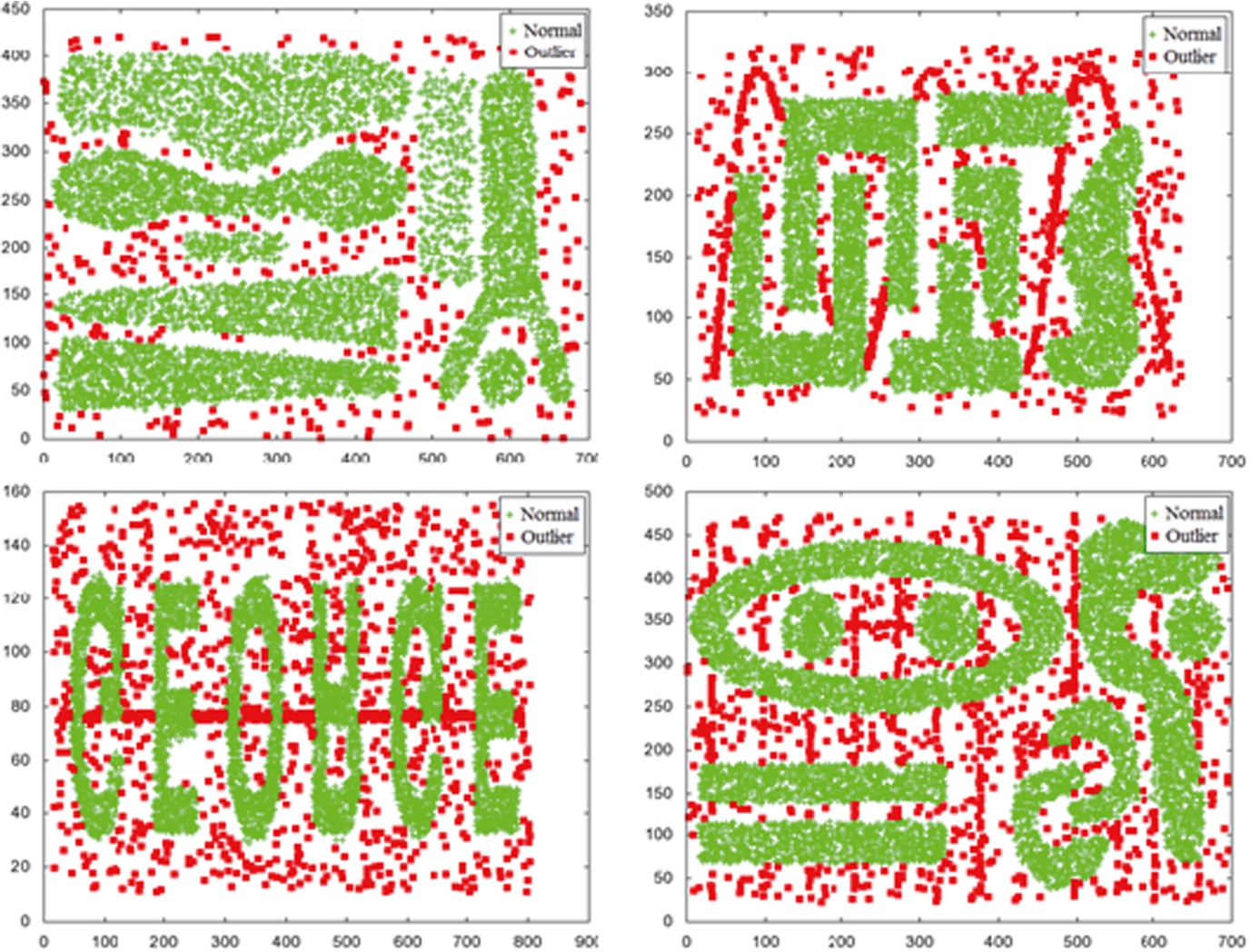
For experiments, we used (1) the well-known four 2-dimensional synthetic datasets used in Chameleon (Karypis et al., 1999) and (2) one real-world dataset composed of the records of the NBA players (Basketball-Reference.com). The Chameleon datasets are composed of 8,000, 8,000, 8,000, and 10,000 objects, respectively, as shown in Fig. 10. The NBA dataset is composed of statistics of 585 basketball players with 23 attributes in the 2004–2005 NBA regular season.
We used the precision, recall, and the execution time as our evaluation metrics. The precision and recall are calculated as follows:
(6)
(7)
All the experiments performed in this paper were executed on Intel i7 920 with 16 GB RAM running Windows 7, and the programs were coded in C#.
6.2Qualitative Analysis
We first conducted a toy experiment to show that our proposed method works for the problems mentioned earlier. For this purpose, we synthetically generated a small 2-dimentional dataset. The dataset contains two clusters (each with fringe objects and different densities), a micro-cluster, and a few randomly generated outlier objects. The dataset is composed of 266 objects and 29 outliers.
Figure 11 shows the dataset and the result of our proposed method on it. We used
Fig. 11
Result of the proposed outlier detection method.
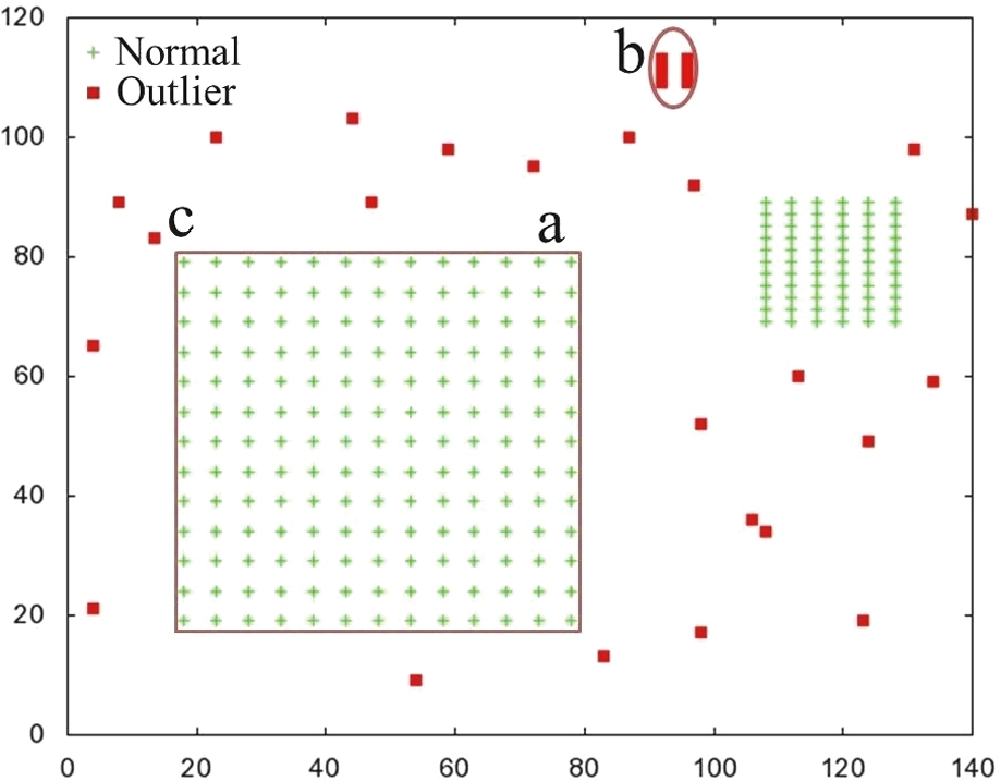
Fig. 12
Precision with varying graph modelling schemes.
We also detected outliers using k-Dist (Ramaswamy et al., 2000) (distance-based) and LOF (Breunig et al., 2000) (density-based) methods. As a result, not surprisingly, all the three problems mentioned above occurred in the k-Dist method and the two problems except for the local density problem occurred in the LOF method.
6.3Analysis on the Proposed Outlier Detection Method
In this subsection, we used the four Chameleon datasets to evaluate the precision of our method while changing (1) graph modelling schemes, (2) weight assignment methods, and (3) the number of iterations (MAX_ITERATIONS).
6.3.1Analysis on Graph Modelling Schemes
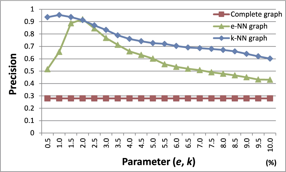
In this experiment, we compare the three different graph modelling schemes we discussed in Section 5.1: (1) complete graph, (2) e-NN graph, and (3) k-NN graph. We used Chameleon datasets to build graphs with each modelling scheme. After building graphs, we detected outliers using our proposed method while varying parameter e of the e-NN graph from 0.5% to 10% in step of 0.5% of the furthest distance between two objects in the dataset. Also, the parameter k of the k-NN graph was varied from 0.5% to 10% in steps of 0.5% of the total number of objects in the dataset, respectively.
A weight on each edge was assigned using the Euclidean similarity, and the number of outliers to be detected was set as equal to the number of outliers selected by humans in each dataset.
Figure 12 shows the results. The x-axis indicates the parameter value of each modelling scheme and the y-axis shows the precision. The complete graph shows the lowest precision. In case of the e-NN graph, the fluctuation of the precision is very large according to the change of e. The k-NN graph, compared to the other graph modelling schemes, shows the highest precision and shows a much smaller fluctuation of the precision according to the parameter change than the e-NN graph.
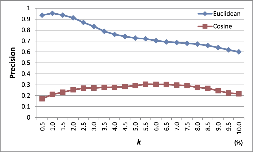
6.3.2Analysis on Weight Assignment Methods
In this experiment, we first modelled the four Chameleon datasets as k-NN graphs and assigned edge weights using (1) the Euclidean similarity and (2) the cosine similarity. Then, we measured the average precision of our method with a varying parameter k in the k-NN graph from 0.5% to 10% in steps of 0.5% of the total number of objects in the dataset. The number of outliers to be detected was set as equal to the number of outliers selected by humans in each dataset.
Figure 13 shows the results. The Euclidean similarity method shows superior precision to the cosine similarity method. In the case of the cosine similarity, even for two distant objects, if the cosine value between their corresponding vectors is 0, a high weight is assigned to the edge connecting the two objects. This could make our method unable to accurately detect outliers.
Fig. 13
Precision with varying weight assignment methods.
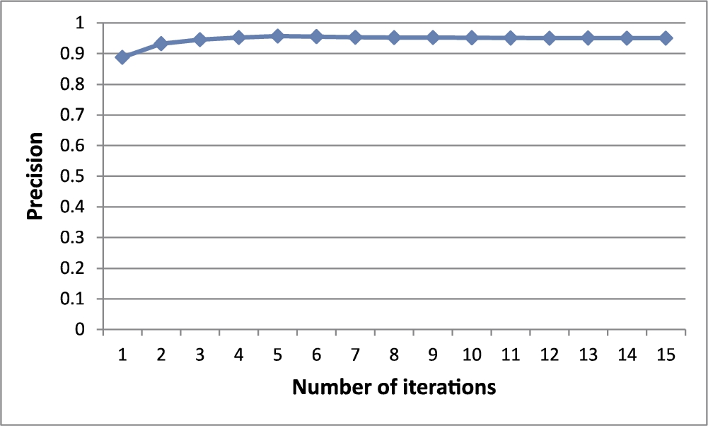
6.3.3Analysis on the Numbers of Iterations
In this experiment, we measured the average precision of our method changing the number of iterations (MAX_ ITERATIONS) from 1 to 15 for calculating centrality and centre-proximity scores. The four Chameleon datasets were modelled as k-NN graphs and the edge weights were assigned by the Euclidean similarity method. Here, k was set as the value providing the best precision for each dataset, as shown in Fig. 12. Also, in order to measure the precision, the number of outliers to be detected was set as equal to the number of true outliers shown by humans in the dataset.
Figure 14 shows the results. The precision increases as the number of iterations increases. When the number of iterations exceeds 5 or 6, both the centrality and centre-proximity scores of all the objects converge to a specific value and the precision does not change. So, we know that the actual execution time of outlier detection by our method is not that large.
Fig. 14
Precision with a varying number of iterations.
6.4Comparisons with Other Methods
In this experiment, we evaluated the average precision and the average execution time of five different outlier detection methods, k-Dist (Ramaswamy et al., 2000) (distance-based), LOF (Breunig et al., 2000) (density-based), Outrank-a, Outrank-b (RWR-based), and the proposed method. For this evaluation, we used four Chameleon datasets. For each method, we select the parameter values (e.g. k for k-NN graph), among multiple candidate values, that provide the best precision.
6.4.1Precision
In this experiment, we used the Chameleon datasets to show the effectiveness of our proposed method by average precisions. We compare our method to the existing outlier detection methods. The parameters for the existing methods were set to the same values as in their papers that showed the best precision for each dataset (Knorr et al., 2000; Moonesinghe and Tan, 2008; Ramaswamy et al., 2000; Breunig et al., 2000).
Table 1 shows the results. Our proposed method that takes account of the distribution of all the objects showed the best average precision. The density-based outlier detection method (LOF) that only takes account of the influence of the neighbouring objects showed a higher precision than the distance-based outlier detection method (k-Dist) that only takes account of the influence of the target object itself. The Outrank methods basically use a concept similar to the proposed method in terms of modelling a given dataset as a graph. However, they have problems in their location features and in the graph modelling schemes, which leads to a very low precision.
Table 1
Precision of five different methods.
| k-Dist | LOF | Outrank-a | Outrank-b | Proposed method | |
| data1 | 0.70 | 0.85 | 0.07 | 0.09 | 0.88 |
| data2 | 0.88 | 0.85 | 0.13 | 0.23 | 0.86 |
| data3 | 0.94 | 0.94 | 0.12 | 0.17 | 0.95 |
| data4 | 0.91 | 0.89 | 0.18 | 0.15 | 0.91 |
| Average | 0.86 | 0.88 | 0.13 | 0.16 | 0.90 |
6.4.2Execution Time
In this experiment, we measured the average execution time of five different outlier detection methods over the four Chameleon datasets. To remove randomness effects, we executed them five times and calculated the average execution times. Here, the parameters of each outlier detection method were set to the values that showed the best precision for each dataset.
Table 2 shows the results in the unit of microseconds (ms). The proposed method, which takes account of the characteristics of all the objects and shows the highest precision, does not show any big difference in terms of the execution time compared to other outlier detection methods.
In case of the Outrank-a method, the given dataset is modelled as a complete graph. Thus, it was shown to require a lot of time to detect the outliers. In case of the Outrank-b method, the execution time of the sharing neighbourhood similarity measure (Ramaswamy et al., 2000), which assigns the edge weight in the Outrank-b method, takes a huge amount of time. Thus, its overall execution time was shown to be very large.
Table 2
Execution time of five different methods (
| k-Dist | LOF | Outrank-a | Outrank-b | Proposed method | |
| data1 | 56,447 | 52,510 | 408,352 | 9,730,417 | 56,515 |
| data2 | 55,913 | 54,718 | 402,726 | 7,951,859 | 57,029 |
| data3 | 56,054 | 54,409 | 403,579 | 7,836,638 | 57,214 |
| data4 | 86,974 | 89,522 | 673,850 | 19,130,638 | 87,340 |
| Average | 63,847 | 62,790 | 472,127 | 11,162,388 | 64,525 |
6.5Detecting Outliers from a Real-World Dataset
In this experiment, we applied our proposed outlier detection method to a real-world dataset. The dataset is composed of the statistics of 585 basketball players in the 2004–2005 NBA regular season. From the NBA dataset, we derived the attributes as shown in Table 3. To derive the attributes, we used the formulas provided in ESPN (ESPN Fantasy Basketball). We normalized the domain of each attribute in order to prevent the situation where the domain of a specific attribute is very large. The attribute a of object v was normalized using the formula
Table 3
Derived attributes from the NBA 2004 dataset.
| Derived attributes | Description | Formula |
| FG% | Field goal percentage | #field goals made #field goals attempted |
| FT% | Free throw percentage | #free throws made #free throws attempted |
| 3P% | Three-point percentage | #three-point goals made / #three-point goals attempted |
| ASTPG | #assists per game | #assists / #played games |
| BLKPG | #blocks per game | #blocks / #played games |
| MINPG | Minutes per game | Minutes of played game / #played games |
| PTSPG | Points per game | Points / Number of played games |
| REBPG | #rebounds per game | #rebounds / #played games |
| STLPG | #steals per game | #steals / #played games |
| TOPG | #turnovers per game | #turnovers / #played games |
We set
Table 4
Top 15 outlier 2004 NBA players.
| fname | lname | team | gp | min | FG% | FT% | 3P% | ASTPG | BLKPG | MINPG | PTSPG | REBPG | STLPG | TOPG |
| Steve | Nash | PHO | 75 | 2,573 | 0.78 | 0.94 | 1.14 | 5.61 | −0.63 | 1.38 | 1.31 | −0.05 | 0.79 | 2.73 |
| Andrei | Kirilenko | UTA | 41 | 1,349 | 0.69 | 0.44 | 0.43 | 0.85 | 6.00 | 1.24 | 1.32 | 1.16 | 2.23 | 1.34 |
| Allen | Iverson | PHI | 75 | 3,174 | −0.01 | 0.69 | 0.48 | 3.59 | −0.55 | 2.15 | 3.86 | 0.23 | 3.93 | 4.44 |
| Jimmy | Jackson | PHO | 40 | 997 | 0.100 | 1.30 | 1.30 | 0.40 | −0.59 | 0.46 | 0.17 | 0.18 | −0.73 | 0.41 |
| Larry | Hughes | WAS | 61 | 2,358 | 0.05 | 0.41 | 0.34 | 1.69 | −0.19 | 1.80 | 2.41 | 1.18 | 5.00 | 1.75 |
| Shaun | Livingston | LAC | 30 | 812 | −0.12 | 0.25 | −1.19 | 1.90 | −0.04 | 0.67 | −0.06 | −0.19 | 0.97 | 1.74 |
| Ruben | Patterson | POR | 70 | 1,957 | 1.08 | −0.46 | −0.76 | 0.14 | −0.18 | 0.76 | 0.64 | 0.20 | 1.96 | 1.14 |
| Greg | Buckner | DEN | 70 | 1,522 | 1.05 | 0.41 | 1.00 | 0.09 | −0.62 | 0.16 | −0.27 | −0.19 | 0.98 | −0.60 |
| Reggie | Evans | SEA | 79 | 1,881 | 0.52 | −0.78 | −1.19 | −0.58 | −0.40 | 0.36 | −0.49 | 2.45 | 0.24 | 0.20 |
| Ben | Wallace | DET | 74 | 2,672 | 0.29 | −1.3 | −0.59 | −0.04 | 4.08 | 1.55 | 0.33 | 3.65 | 1.78 | −0.10 |
| Ervin | Johnson | MIN | 46 | 410 | 0.96 | −0.26 | 4.22 | −0.92 | −0.21 | −1.09 | −1.04 | −0.41 | −1.05 | −1.00 |
| Kevin | Garnett | MIN | 82 | 3,121 | 0.79 | 0.57 | 0.11 | 2.27 | 2.00 | 1.74 | 2.43 | 4.20 | 1.88 | 2.01 |
| Eddie | Griffin | MIN | 70 | 1,492 | −0.39 | 0.12 | 0.59 | −0.56 | 2.66 | 0.11 | −0.04 | 1.27 | −0.66 | −0.49 |
| Darius | Miles | POR | 63 | 1,698 | 0.58 | −0.46 | 0.69 | 0.18 | 1.74 | 0.66 | 0.85 | 0.55 | 1.25 | 1.73 |
| Anthony | Carter | MIN | 66 | 742 | −0.19 | −0.04 | −0.55 | 0.41 | −0.23 | −0.86 | −0.85 | −0.99 | −0.22 | −0.29 |
The outliers detected in the NBA dataset not only include the outstanding players but also may include the players that have poor statistics. Steve Nash, the 3rd outlier, is shown 5.61 times higher in assists per game compared with the average of other players. Andrei Kirilenko, the 4th outlier, is shown 6 times higher in blockings per game compared with the average of other players. Additionally, the best players such as Allen Iverson (top player in points), Larry Hughes (top player in steals), and Kevin Garnet (top player in rebounds) were all included in the top 25.22 Other players who were detected as outliers either have poor statistics or did not play in many games.
7Conclusions and Future Work
After extensive analysis of existing outlier detection methods we noticed their significant lack and problems that can cause wrong interpretation of obtained experimental results with different datasets. Our intention in recent research was to propose a novel method that would show better effects and performances. In this paper, we have proposed a novel outlier detection method based on centrality and centre-proximity notions. Apart from that, we proposed a graph-based outlier detection method and presented extensive promising experimental results.
The main contributions of our research presented in this paper could be summarized as follows: (1) We have proposed two novel relative location features–centrality and centre-proximity. Both features take account of the characteristics of all the objects in the dataset. (2) To solve the local density and micro-cluster problems, we have proposed a novel graph-based outlier detection method. (3) We have explored multiple graph modelling schemes and weighting schemes for our graph-based outlier detection. (4) The effectiveness and efficiency of the proposed method have been verified in extensive experiments with both synthetic and real-world datasets. Comparison with previous methods has been discussed and the advantages of our approach have been specified.
Based on promising and positive effects we obtained in experiments, we are going to continue with additional experiments and enhance our efforts in comparative evaluations with more sophisticated competitors (e.g. neural networks and probabilistic methods) and more datasets including benchmark datasets.
Notes
1 A preliminary version of this work has been presented as a poster (4 pages) in ACM CIKM 2012 (Bae et al., 2012). This paper has additional contributions compared with its preliminary version listed as follows: (1) we define four goals of the proposed method to clarify its advantages; (2) we propose three graph models for our method and compare their effectiveness via extensive experiments; (3) we propose two weighting schemes for our method and compare their effectiveness via extensive experiments; (4) we show the results obtained by applying the proposed method to a real-world NBA dataset; (5) we show the superiority of the proposed method over more competitors.
References
1 | Akoglu, L., McGlohon, M., Faloutsos, C. ((2010) ). OddBall: spotting anomalies in weighted graphs. In: Proceedings of the 14th Pacific-Asia Conference on Advances in Knowledge Discovery and Data Mining, pp. 410–421. |
2 | Bae, D.-H., Jeong, S., Kim, S.-W., Lee, M. ((2012) ). Outlier detection using centrality and center-proximity. In: Proceedings of the 21st ACM International Conference on Information and Knowledge Management, pp. 2251–2254. |
3 | Barnett, V., Lewis, T. ((1994) ). Outliers in Statistical Data. John Wiley & Sons. |
4 | Bay, S.D., Schwabacher, M. ((2003) ). Mining distance-based outliers in near linear time with randomization and a simple pruning rule. In: Proceedings of the 9th ACM SIGKDD International Conference on Knowledge Discovery and Data Mining, pp. 29–38. |
5 | Böhm, C., Haegler, K., Müller, N.S., Plant, C. ((2009) ). CoCo: coding cost for parameter-free outlier detection. In: Proceedings of the 15th ACM SIGKDD International Conference on Knowledge Discovery and Data Mining, pp. 149–158. |
6 | Breunig, M.M., Kriegel, H.P., Ng, R.T., Sander, J. ((2000) ). LOF: identifying density-based local outliers. In: Proceedings of the 2000 ACM SIGMOD International Conference on Management of Data, pp. 93–104. |
7 | Brin, S., Page, L. ((1998) ). The anatomy of a large-scale hypertextual Web search engine. In: Proceedings of the 7th International World Wide Web Conference, pp. 107–117. |
8 | Chan, K.Y., Kwong, C.K., Fogarty, T.C. ((2010) ). Modeling manufacturing processes using a genetic programming-based fuzzy regression with detection of outliers. Information Sciences, 180: (4), 506–518. |
9 | Chandola, V., Banerjee, A., Kumar, V. ((2009) ). Anomaly detection: a survey. ACM Computing Surveys, 41: (3), 15:1–15:58. |
10 | Domingues, R., Filippone, M., Michiardi, P., Zouaoui, J. ((2018) ). A comparative evaluation of outlier detection algorithms: experiments and analyses. Pattern Recognition, 74: , 406–421. |
11 | Fanaee-T, H., Gama, J. ((2016) ). Tensor-based anomaly detection: an interdisciplinary survey. Knowledge-Based Systems, 98: , 130–147. |
12 | Friedman, M., Last, M., Makover, Y., Kandel, A. ((2007) ). Anomaly detection in web documents using crisp and fuzzy-based cosine clustering methodology. Information Sciences, 177: (2), 467–475. |
13 | Ha, J., Bae, D.-H., Kim, S.-W., Baek, S.C., Jeong, B.S. ((2011) ). Analyzing a Korean blogosphere: a social network analysis perspective. In: Proceedings of the 2011 ACM Symposium on Applied Computing, pp. 773–777. |
14 | Han, J., Kamber, M. ((2000) ). Data Mining: Concepts and Techniques. Morgan Kaufmann. |
15 | Hawkins, D.M. ((1980) ). Identification of Outliers. Chapman and Hall. |
16 | Huang, J., Zhu, Q., Yang, L., Feng, J. ((2016) ). A non-parameter outlier detection algorithm based on natural neighbor. Knowledge-Based Systems, 92: , 71–77. |
17 | Karypis, G., Han, E.H., Kumar, V. ((1999) ). Chameleon: hierarchical clustering using dynamic modeling. IEEE Computer, 32: (8), 68–75. |
18 | Kieu, T., Yang, B., Jensen, C.S. ((2018) ). Outlier detection for multidimensional time series using deep neural networks. In: Proceedings of the 19th IEEE International Conference on Mobile Data Management, pp. 125–134. |
19 | Kleinberg, J.M. ((1999) ). Authoritative sources in a hyperlinked environment. Journal of the ACM, 46: (5), 604–632. |
20 | Knorr, E.M., Ng, R.T. ((1999) ). Finding intensional knowledge of distance-based outliers. In: Proceedings of 25th International Conference on Very Large Data Bases, pp. 211–222. |
21 | Knorr, E.M., Ng, R.T., Tucakov, V. ((2000) ). Distance-based outliers: algorithms and applications. The VLDB Journal, 8: (3–4), 237–253. |
22 | Moonesinghe, H.D.K., Tan, P.N. ((2008) ). OutRank: a graph-based outlier detection framework using random walk. International Journal on Artificial Intelligence Tools, 17: (01), 19–36. |
23 | Na, G.S., Kim, D., Yu, H. ((2018) ). DILOF: effective and memory efficient local outlier detection in data streams. In: Proceedings of the 24th ACM SIGKDD International Conference on Knowledge Discovery & Data Mining, pp. 1993–2002. |
24 | Papadimitriou, S., Kitagawa, H., Gibbons, P.B., Faloutsos, C. ((2003) ). LOCI: fast outlier detection using the local correlation integral. In: Proceedings of the 19th International Conference on Data Engineering, pp. 315–326. |
25 | Ramaswamy, S., Rastogi, R., Shim, K. ((2000) ). Efficient algorithms for mining outliers from large data sets. SIGMOD Record, 29: (2), 427–438. |
26 | Song, J., Takakura, H., Okabe, Y., Nakao, K. ((2013) ). Toward a more practical unsupervised anomaly detection system. Information Sciences, 231: , 4–14. |
27 | Tan, P.N., Steinbach, M., Kumar, V. ((2005) ). Introduction to Data Mining. Addison-Wesley. |
28 | Widyantoro, D.H., Ioerger, T.R., Yen, J. ((2002) ). An incremental approach to building a cluster hierarchy. In: Proceedings of the 2002 IEEE International Conference on Data Mining, pp. 705–708. |
29 | Yerlikaya-Ö, F., Askan, A., Weber, G.W. ((2016) ). A hybrid computational method based on convex optimization for outlier problems: application to earthquake ground motion prediction. Informatica, 27: (4), 893–910. |
30 | Basketball-Reference.com. Available from: http://www.basketball-reference.com/. |
31 | ESPN Fantasy Basketball. Available from: http://www.espn.com/fantasy/basketball/. |


