Applications of Edge Colouring of Fuzzy Graphs

1Introduction

The concept of fuzzy graph, introduced by Kauffman (1973) initially, was interpreted by Rosenfeld (1975). Samanta and Pal (2015, 2013) introduced different types of fuzzy graphs. For further details about the fuzzy graphs, readers may see Mordeson and Nair (2000), Samanta et al. (2016a), Sarkar and Samanta (2017), Mahapatra et al. (2019a). Early in the literature, one of the useful problems, the traffic light problem, was solved using the crisp graph colouring technique. But, in traffic light problems, some routes are busier compared to the other routes. Also, sometimes, two routes are open simultaneously with some caution. Here “busy”, “caution” are fuzzy terms. So fuzzy/uncertainty could be included in the traffic light problem. Munoz et al. (2005) designed the traffic light problem by fuzzy graphs and introduced the method of colouring in fuzzy graphs. The edge colouring of fuzzy graphs could demonstrate the traffic light problem properly. The membership value of edges is calculated from the congestion of the route and the probability of accidents. If the signal lights are based on these membership values and used alongside the fuzzy colour, the density of the signal colours could indicate the flow of traffic in a particular region. In that paper, the fuzzy graphs were considered with crisp vertices and fuzzy edges. Then α-cuts Mordeson and Nair (2000) of these fuzzy graphs were coloured according to the method of the crisp graph colouring. Thus, for different values of α, there are different crisp graphs, and these crisp graphs are coloured. Therefore, the chromatic index varies for the same fuzzy graphs for different values of α. Also, Bershtein and Bozhenuk (2001) proposed a different technique to colour fuzzy graphs. In this paper, a term separation degree of fuzzy graphs has been defined and based on the value of separation degree, the number of minimum colour is found. Vertex colouring on fuzzy graphs is applied for map colouring Samanta et al. (2016b). Recently, major developments on chromatic index on fuzzy graphs are obtained from the papers of Rosyida et al. (2016, 2015) and Chen et al. (2017). Kishore and Sunitha Kishore and Sunitha (2014, 2016) introduced chromaticity and strong chromaticity of fuzzy graphs. Mahapatra et al. (2019b) advanced the colouring concept to radio fuzzy graphs and resolved radio frequency problems.

Sometimes, the relationship (edges) is more meaningful than the people (nodes). For example, the links in fuzzy social networks are more important than the nodes. Thus, it is essential to show the fuzzy links properly by colouring. Edge colouring, a related term, is important to the problems which are based on uncertainty. In Section 3 of this paper, edge colouring of fuzzy graphs is introduced. After that, in Section 4, chromatic index of fuzzy graphs, an associated term of graph colouring, is defined. Based on this technique, the number of basic colours is counted. In fuzzy graphs, edge colourings use colour density. Sometimes, deep/strong colours are to be used to emphasize the importance of the corresponding relation/edge. The definition of strong chromatic index is updated in Section 6. Here, a recruiting web site is represented from both companies’ and candidates’ point of view by edge colouring of fuzzy graphs in Section 6. Traffic light problems have been modified and solved in Section 7. At last, a conclusion is drawn in Section 8.

2Preliminaries

A graph is defined as a pair G∗=(V,E)[TeX:] ${G^{\ast }}=(V,E)$, where V is the set, and E is a relation on V. The elements of V are called vertices, and the elements of E are called edges of G∗[TeX:] ${G^{\ast }}$.

A fuzzy set A on a universal set X is characterized by a mapping m:X→[0,1][TeX:] $m:X\to [0,1]$, which is called the membership function. A fuzzy set is denoted by A=(X,m)[TeX:] $A=(X,m)$.

A fuzzy graph Rosenfeld (1975) ξ=(V,σ,μ)[TeX:] $\xi =(V,\sigma ,\mu )$ is a non-empty set V together with a pair of functions σ:V→[0,1][TeX:] $\sigma :V\to [0,1]$ and μ:V×V→[0,1][TeX:] $\mu :V\times V\to [0,1]$, such that for all x,y∈V[TeX:] $x,y\in V$, [μ(x,y)⩽min{σ(x),σ(y)}][TeX:] $[\mu (x,y)\leqslant \min \{\sigma (x),\sigma (y)\}]$, where σ(x)[TeX:] $\sigma (x)$ and μ(x,y)[TeX:] $\mu (x,y)$ represent the membership values of the vertex x and of the edge (x,y)[TeX:] $(x,y)$ in ξ, respectively.

A path in a fuzzy graph is a sequence of distinct nodes x0,x1,…,xn[TeX:] ${x_{0}},{x_{1}},\dots ,{x_{n}}$, such that μ(xi−1,xi)>0,1⩽i⩽n[TeX:] $\mu ({x_{i-1}},{x_{i}})>0,1\leqslant i\leqslant n$. The fuzzy path is said to be fuzzy cycle if x0[TeX:] ${x_{0}}$ and xn[TeX:] ${x_{n}}$ coincide.

The strength of a path is the minimum membership value of an edge in the path. The maximum of all strengths of paths between two vertices is the strength of connectivity between the vertices.

The underlying crisp graph of the fuzzy graph ξ=(V,σ,μ)[TeX:] $\xi =(V,\sigma ,\mu )$ is denoted as ξ=(V,σ,μ)[TeX:] $\xi =(V,\sigma ,{\mu ^{)}}$ where σ={u∈V|σ(u)>0}[TeX:] $\sigma =\{u\in V|\sigma (u)>0\}$ and μ={(u,v)∈V×V|μ(u,v)>0}[TeX:] $\mu =\{(u,v)\in V\times V|\mu (u,v)>0\}$. Thus, for underlying fuzzy graph, σ=V[TeX:] $\sigma =V$ is true.

A fuzzy graph ξ=(V,σ,μ)[TeX:] $\xi =(V,\sigma ,\mu )$ is complete if μ(u,v)=min{σ(u),σ(v)}[TeX:] $\mu (u,v)=\min \{\sigma (u),\sigma (v)\}$ for all u,v∈V[TeX:] $u,v\in V$, where (u,v)[TeX:] $(u,v)$ denotes the edge between the vertices u and v.

A fuzzy graph ξ=(V,σ,μ)[TeX:] $\xi =(V,\sigma ,\mu )$ is said to be bipartite if the vertex set V can be partitioned into two nonempty sets V1[TeX:] ${V_{1}}$ and V2[TeX:] ${V_{2}}$, such that μ(v1,v2)=0[TeX:] $\mu ({v_{1}},{v_{2}})=0$ if v1,v2∈V1[TeX:] ${v_{1}},{v_{2}}\in {V_{1}}$ or v1,v2∈V2[TeX:] ${v_{1}},{v_{2}}\in {V_{2}}$. Furthermore, if μ(v1,v2)=min{σ(v1),σ(v2)}[TeX:] $\mu ({v_{1}},{v_{2}})=\min \{\sigma ({v_{1}}),\sigma ({v_{2}})\}$ for all v1∈V1[TeX:] ${v_{1}}\in {V_{1}}$ and v2∈V2[TeX:] ${v_{2}}\in {V_{2}}$, then ξ is called a fuzzy complete bipartite graph.

3Edge Colouring of Fuzzy Graphs

Samanta et al. (2016b) defined fuzzy colours as mixed colours. But when a colour is mixed with white, its intensity is reduced. Now, intensity is a fuzzy term. Suppose β (⩽1)[TeX:] $(\leqslant 1)$ units of the colour ck[TeX:] ${c_{k}}$ are mixed with 1−β[TeX:] $1-\beta $ units of white colour, then the mixture is called a standard mixture of the colour ck[TeX:] ${c_{k}}$. The resulted colour is called the fuzzy colour of the colour ck[TeX:] ${c_{k}}$ with membership value β, whereas ck[TeX:] ${c_{k}}$ is called the basic colour. For example, red, black, green, etc. are basic colours. The definition of fuzzy colour is given as follows.

Hence, the colour (wi,h(wi))[TeX:] $({w_{i}},h({w_{i}}))$ is called the fuzzy colour corresponding to the basic colour wi[TeX:] ${w_{i}}$. Thus, h(wi)[⩽1][TeX:] $h({w_{i}})[\leqslant 1]$ amount of wi[TeX:] ${w_{i}}$ is mixed with 1−h(wi)[TeX:] $1-h({w_{i}})$ amount of white colour to form the fuzzy colour (wi,h(wi))[TeX:] $({w_{i}},h({w_{i}}))$.

According to the above definition of fuzzy colour, different fuzzy colours are constructed from a basic colour. For example, red is a basic colour. A “fuzzy red” colour may be formed from red by mixing 0.9 units of red colour with 0.1 units of white colour. This “fuzzy red” colour is denoted by (red,0.9)[TeX:] $(\mathit{red},0.9)$. Similarly, another fuzzy red colour (red,0.75)[TeX:] $(\mathit{red},0.75)$ may be formed by mixing 0.75 units of red colour with 0.25 units of white colour, and so on. Now, these fuzzy colours are used for edge colouring of fuzzy graphs in the following ways.

4Chromatic Index of Fuzzy Graphs

The minimum number of basic colours needed to colour a fuzzy graph is called fuzzy chromatic index of a fuzzy graph. Suppose that such minimum number of basic colours is N. Now, this crisp chromatic index is not sufficient to mention the strengths of edges (i.e. the relationship among vertices). For example, chromatic indexes of two fuzzy graphs are the same. Then it is inconclusive when these graphs are being compared. Hence, the chromatic index is associated with some weight. The weight is denoted by W, and defined by W=∑i=1N{maxjfej(ci)}[TeX:] $W={\textstyle\sum _{i=1}^{N}}\{{\max _{j}}{f_{{e_{j}}}}({c_{i}})\}$. Where the basic colour ci[TeX:] ${c_{i}}$ is used to colour the edge ej[TeX:] ${e_{j}}$ for some j, and depth of colour is fej(ci)[TeX:] ${f_{{e_{j}}}}({c_{i}})$. Thus, W is the sum of the maximum membership values of each basic colour. Now, the chromatic index of a fuzzy graph is denoted by (N,W)[TeX:] $(N,W)$, where N is the minimum number of basic colours to colour a graph, and W is its weight. It is obvious that the weight of the chromatic index is to be determined by decision makers for a particular case.

4.1Algorithm of Minimum Colouring of Edges of a Fuzzy Graph

Input: A fuzzy graph ξ=(V,σ,μ)[TeX:] $\xi =(V,\sigma ,\mu )$, |V|=n[TeX:] $|V|=n$. Assume that the vertices are labelled as 1,2,…,n[TeX:] $1,2,\dots ,n$.

Output: Complete a edge coloured graph.

Step 1: Now, f-value (fej(ci)=μ(u,v)σ(u)∧σ(v)[TeX:] ${f_{{e_{j}}}}({c_{i}})=\frac{\mu (u,v)}{\sigma (u)\wedge \sigma (v)}$) of all edges are to be calculated.

Step 2: First of all, the vertex “1” is targeted to colour all its incident edges in such a way that the minimum number of colours would be used. Hence, if one colour is used, a different colour is to be used only if the edges are incident to the vertex.

Step 3: Proceed to direct neighbours of “1” except the previous one which is already focused and label them 11,12,…,1m[TeX:] $11,12,\dots ,1m$, if there are m-such neighbours. Start with the vertex 11 and repeat Step 2 and so on for 12,13,…,1m[TeX:] $12,13,\dots ,1m$.

Step 4: Repeat Step 3 until all edges of the graph have been coloured.

Formally, the definition of chromatic index for fuzzy graphs is given as follows. The concept of this chromatic index will allow to mention the weight of edge colouring.

Definition 2.

Let G=(V,σ,μ)[TeX:] $G=(V,\sigma ,\mu )$ be a fuzzy graph. The order pair (N,W)[TeX:] $(N,W)$ is said to be the chromatic index of G where N is the minimum number of colour needed to colour the graph G and W=∑i=1N{maxjfej(ci)}[TeX:] $W={\textstyle\sum _{i=1}^{N}}\{ma{x_{j}}{f_{{e_{j}}}}({c_{i}})\}$, the basic colour ci[TeX:] ${c_{i}}$ is used to colour the edge ej[TeX:] ${e_{j}}$ for some j, and the depth of colour is fej(ci)[TeX:] ${f_{{e_{j}}}}({c_{i}})$.

The chromatic index on fuzzy graphs is a pair whose first element represents the crisp chromatic index, and the second element is its weight. The crisp number indicates only the number of different colours required to colour the edges of a graph while the weight represents the sum of strengths of the edges. This weight is meaningful only when it is of a very high or very low value, i.e. all edges are strong, or all edges are weak. Thus, the weight needs further restrictions.

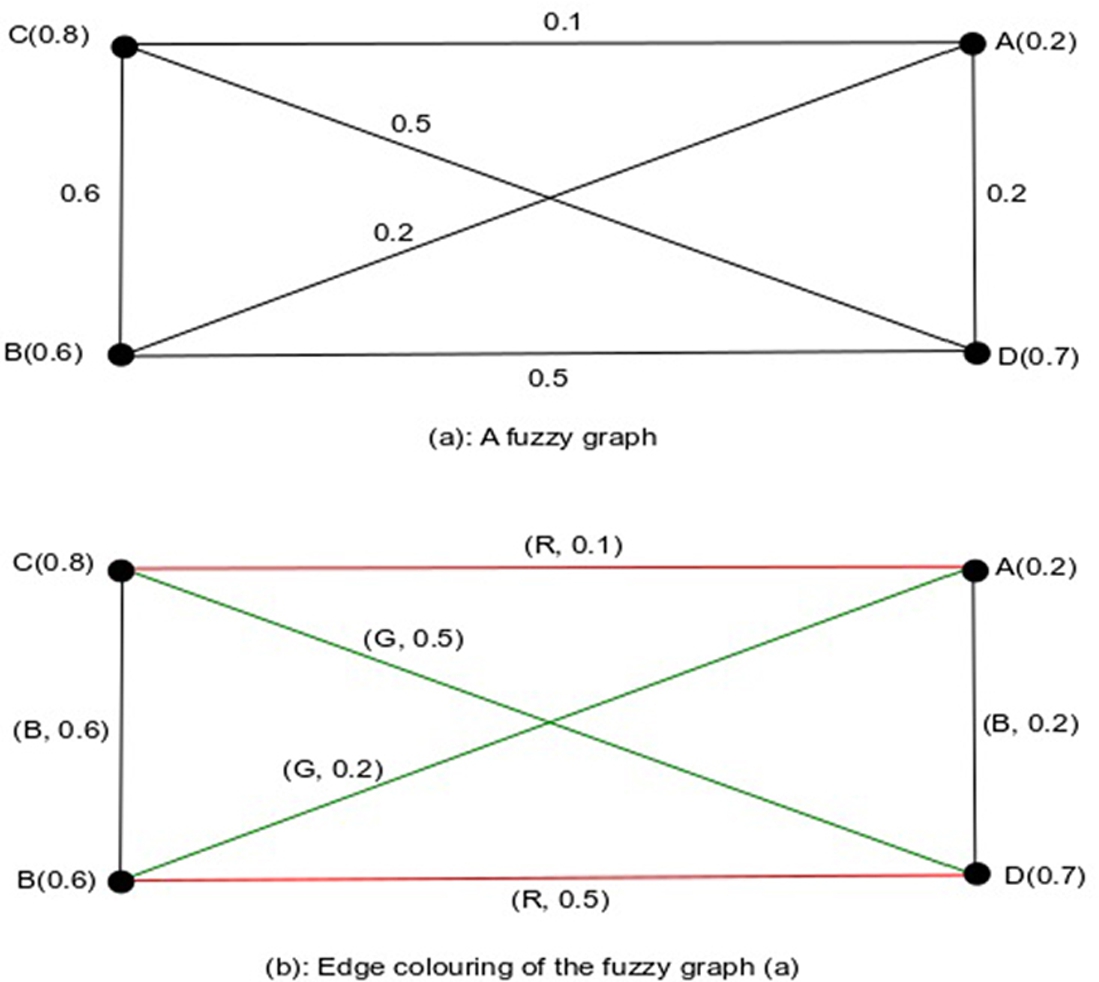
Example 1.

An example is considered in Fig. 1. In this example, three basic colours (red, black and green) are used for the colouring of the fuzzy graph, i.e. N=3[TeX:] $N=3$. The depth of colouring is the strength of the corresponding edge. Here, red colour is given in the edges CA[TeX:] $\mathit{CA}$ and BD[TeX:] $\mathit{BD}$ with membership values 0.5 and 0.83 of the edge, respectively. The black colour is assigned to the edges BC[TeX:] $\mathit{BC}$ and AD[TeX:] $\mathit{AD}$ with membership value 1. The green colour is given to the edges CD[TeX:] $CD$ and AB[TeX:] $\mathit{AB}$ with membership values 1 and 0.71, respectively. So the weight W=0.83+1+1=2.83[TeX:] $W=0.83+1+1=2.83$. Thus, the chromatic index of this fuzzy graph is (3,2.83)[TeX:] $(3,2.83)$.

Fig. 1

Edge colouring of fuzzy graphs.

Lemma 1.

Chromatic index of a complete graph is (N,N)[TeX:] $(N,N)$.

Proof.

Let ξ=(V,σ,μ)[TeX:] $\xi =(V,\sigma ,\mu )$ be a complete fuzzy graph, then μ(x,y)=σ(x)∧σ(y)[TeX:] $\mu (x,y)=\sigma (x)\wedge \sigma (y)$. Thus, the membership value of each basic colour must be μ(x,y)σ(x)∧σ(y)=1[TeX:] $\frac{\mu (x,y)}{\sigma (x)\wedge \sigma (y)}=1$. Since the graph is complete, N basic colour is required. Here, the membership value of each basic colour is 1. Then the weight of the chromatic index is {1+1+1+⋯Ntimes}=N[TeX:] $\{1+1+1+\cdots N\hspace{2.5pt}\text{times}\}=N$. So, the chromatic index of a complete graph is (N,N)[TeX:] $(N,N)$.  □

Lemma 2.

If the chromatic index of a fuzzy graph is (N,W)[TeX:] $(N,W)$, then 0<W⩽N[TeX:] $0<W\leqslant N$.

Proof.

Let ξ=(V,σ,μ)[TeX:] $\xi =(V,\sigma ,\mu )$ be a fuzzy graph with a chromatic index (N,W)[TeX:] $(N,W)$. Also, μ(x,y)⩽σ(x)∧σ(y)[TeX:] $\mu (x,y)\leqslant \sigma (x)\wedge \sigma (y)$. It is obvious that the weight W is always positive, i.e. W>0[TeX:] $W>0$. Also, μ(x,y)⩽σ(x)∧σ(y)[TeX:] $\mu (x,y)\leqslant \sigma (x)\wedge \sigma (y)$. Thus, μ(x,y)σ(x)∧σ(y)[TeX:] $\frac{\mu (x,y)}{\sigma (x)\wedge \sigma (y)}$ ⩽ 1. So, the membership value of each colour is smaller or equal to 1. Now W is the sum of membership values of N basic colours. Hence, W⩽N[TeX:] $W\leqslant N$, i.e. 0<W⩽N[TeX:] $0<W\leqslant N$.  □

5Strong Chromatic Index of Edge Colouring of Fuzzy Graphs

The weight of the chromatic number is significant only if the weight is very large or very small. Suppose that two fuzzy graphs have chromatic indexes which are (3,2.9)[TeX:] $(3,2.9)$ and (3,0.3)[TeX:] $(3,0.3)$. It can be said that the edges of the second graph are not strong. But any value which is near about half of its maximum value does not indicate any clear data. The strong chromatic index will be an improved concept of the chromatic index. Let ξ=(V,σ,μ)[TeX:] $\xi =(V,\sigma ,\mu )$ be a connected fuzzy graph. The edges, where μ(x,y)σ(x)∧σ(y)⩾0.5[TeX:] $\frac{\mu (x,y)}{\sigma (x)\wedge \sigma (y)}\geqslant 0.5$, are coloured with fuzzy colours whose membership values are greater than or equal to 0.5. These colours are called strong colours. Strong chromatic index is denoted by γs(ξ)[TeX:] ${\gamma _{s}}(\xi )$ and defined by γs(ξ)=(Ms,Ws)[TeX:] ${\gamma _{s}}(\xi )=({M_{s}},{W_{s}})$, where Ms[TeX:] ${M_{s}}$ is the number of basic colours for colouring of ξ and Ws[TeX:] ${W_{s}}$ is the sum of the membership values of each basic colour. It is assumed that the maximum membership value is taken for the repeated, basic colours.

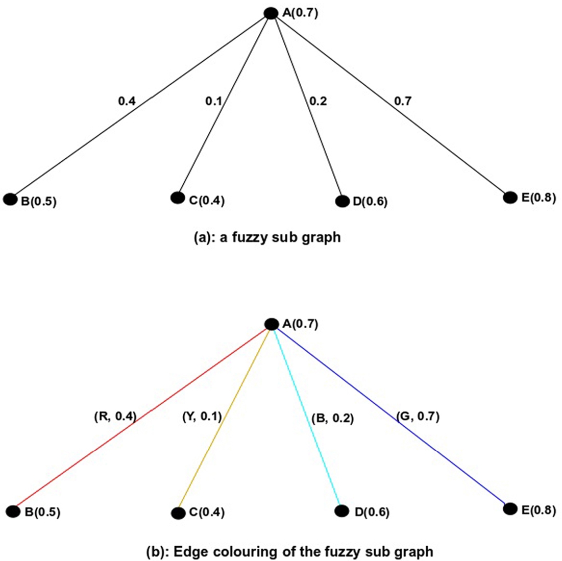
Example 2.

Let us consider a fuzzy graph shown in Fig. 2. Here, four basic colours (red, yellow, green and blue) are used for the colouring of the fuzzy graph. The membership values of the colours are 0.8, 0.25, 0.33, 1, respectively. Therefore, Ms=2[TeX:] ${M_{s}}=2$ and Ws=(0.8+1)=1.8[TeX:] ${W_{s}}=(0.8+1)=1.8$. So, the strong chromatic index of the fuzzy graph is (2,1.8)[TeX:] $(2,1.8)$.

Fig. 2

Colouring of strong edge of fuzzy graphs.

6Representation of Job Oriented Web Sites by Edge Colouring of Fuzzy Graphs

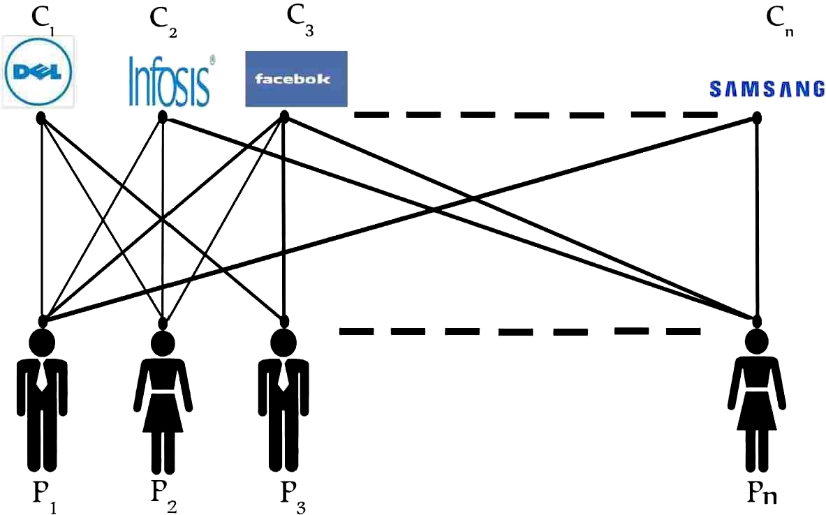
Fuzzy graph colouring problem has various practical applications. One of them is in job oriented web sites. Job oriented web sites are useful in recent years. A lot of recruiters and job seekers gather in these web sites. Fuzzy graphs represent each web site. The following example shows a step by step method of representation of web sites and edge colouring of fuzzy graphs. By looking at the colour of a fuzzy graph, an applicant could understand how many companies suit his/her expertise. Furthermore, on the other side, a company finds a suitable applicant. Thus, the representation of job oriented web sites can be prepared in an easier way using the edge colouring of fuzzy graphs.

Let us assume such a small web site, where N number of candidates are registered for jobs with their Bio-Data, and M number of companies (recruiters) have registered a certain number of vacancies and the brand value of the company for appropriate candidates (see Fig. 3).

If an applicant’s eligibility suits a company’s demand, it is obvious that there exists a relation between them. Here, the companies and candidates are represented as vertices and their links as edges. Now, the membership values of corresponding vertices of the company may depend on the following issues:

The membership values of edges depend on matching the companies’ profiles with the applicants’ profiles. Then, the relationship between companies and applicants is shown as a fuzzy bipartite graph, shown in Fig. 5. If a company wants to find suitable candidates, firstly, it logins into this web site, then it will get a fuzzy subgraph like Fig. 3. The company may shortly find suitable candidates by using the concept of strong chromatic index.

Fig. 3

Representation of companies and applicants in a job oriented web site.

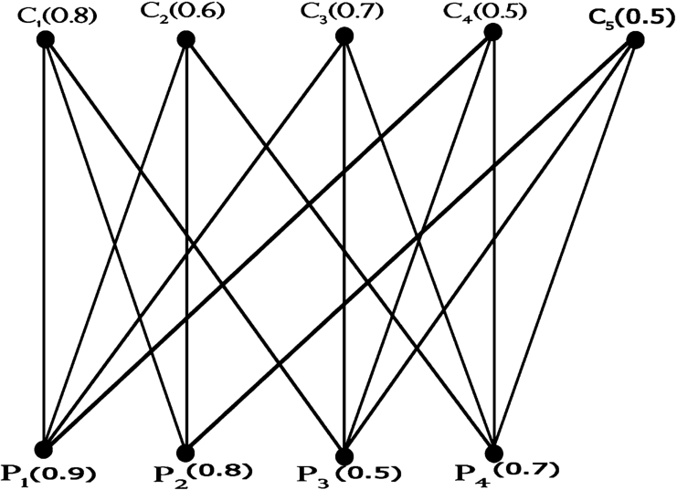
Suppose, in particular, 5 companies and 4 applicants are registered on this job oriented web site (see Fig. 5). Thus, a fuzzy bipartite graph is considered where the vertices are the companies C1,C2,C3,C4,C5[TeX:] ${C_{1}},{C_{2}},{C_{3}},{C_{4}},{C_{5}}$ and the applicants, P1,P2,P3,P4[TeX:] ${P_{1}},{P_{2}},{P_{3}},{P_{4}}$. There is an edge if there exists a particular matching. So the edges are (C1,P1)[TeX:] $({C_{1}},{P_{1}})$, (C1,P2)[TeX:] $({C_{1}},{P_{2}})$,(C1,P3)[TeX:] $({C_{1}},{P_{3}})$, (C2,P1)[TeX:] $({C_{2}},{P_{1}})$, (C2,P2)[TeX:] $({C_{2}},{P_{2}})$, (C2,P4)[TeX:] $({C_{2}},{P_{4}})$, (C3,P1)[TeX:] $({C_{3}},{P_{1}})$, (C3,P3),(C3,P4)[TeX:] $({C_{3}},{P_{3}}),({C_{3}},{P_{4}})$, (C4,P1)[TeX:] $({C_{4}},{P_{1}})$, (C4,P3),(C4,P4)[TeX:] $({C_{4}},{P_{3}}),({C_{4}},{P_{4}})$, (C5,P1)[TeX:] $({C_{5}},{P_{1}})$, (C5,P2)[TeX:] $({C_{5}},{P_{2}})$, (C5,P3)[TeX:] $({C_{5}},{P_{3}})$, (C5,P4)[TeX:] $({C_{5}},{P_{4}})$. The membership value of vertices C1,C2,C3,C4,C5[TeX:] ${C_{1}},{C_{2}},{C_{3}},{C_{4}},{C_{5}}$ depend on the salary, company’s brand value, product value etc., as stated above. The membership values of the vertices P1,P2,P3,P4[TeX:] ${P_{1}},{P_{2}},{P_{3}},{P_{4}}$ depend on qualification, experience, etc., as stated above. The membership values of edges depend on matching the companies with the applicants.

For example, in a particular case, the membership values of vertices C1,C2,C3,C4,C5[TeX:] ${C_{1}},{C_{2}},{C_{3}},{C_{4}},{C_{5}}$ are taken as 0.8,0.6,0.7,0.5,0.5[TeX:] $0.8,0.6,0.7,0.5,0.5$, respectively. The membership values of vertices P1,P2,P3,P4[TeX:] ${P_{1}},{P_{2}},{P_{3}},{P_{4}}$ are considered as 0.9,0.8,0.5,0.7, respectively. Also the membership value of the edges (C1,P1)[TeX:] $({C_{1}},{P_{1}})$, (C1,P2)[TeX:] $({C_{1}},{P_{2}})$, (C1,P3)[TeX:] $({C_{1}},{P_{3}})$, (C2,P1)[TeX:] $({C_{2}},{P_{1}})$, (C2,P2)[TeX:] $({C_{2}},{P_{2}})$, (C2,P4)[TeX:] $({C_{2}},{P_{4}})$, (C3,P1)[TeX:] $({C_{3}},{P_{1}})$, (C3,P3)[TeX:] $({C_{3}},{P_{3}})$, (C3,P4)[TeX:] $({C_{3}},{P_{4}})$, (C4,P1)[TeX:] $({C_{4}},{P_{1}})$, (C4,P3)[TeX:] $({C_{4}},{P_{3}})$, (C4,P4)[TeX:] $({C_{4}},{P_{4}})$, (C5,P1)[TeX:] $({C_{5}},{P_{1}})$, (C5,P2)[TeX:] $({C_{5}},{P_{2}})$, (C5,P3)[TeX:] $({C_{5}},{P_{3}})$, (C5,P4)[TeX:] $({C_{5}},{P_{4}})$ are taken as 0.7, 0.6, 0.5, 0.6, 0.5, 0.4, 0.7, 0.4, 0.6, 0.4, 0.4, 0.5, 0.4, 0.3, 0.2, 0.3, 0.2, respectively.

When a company or an applicant logins into this web site, then they get a fuzzy subgraph like Fig. 5. Particularly, if an applicant P2[TeX:] ${P_{2}}$ logins into this web site, then he/she gets a fuzzy subgraph shown in Fig. 6(a). Also, if a company, in particular, C3[TeX:] ${C_{3}}$ logins into this web site, it gets another fuzzy subgraph shown in Fig. 6(b).

Fig. 4

Fuzzy sub graph for the vertex C2[TeX:] ${C_{2}}$.

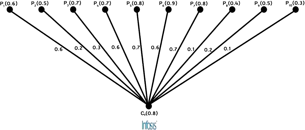
Fig. 5

Fuzzy graph of the job oriented web site.

If these two fuzzy subgraphs are coloured by fuzzy colours, then the applicant P2[TeX:] ${P_{2}}$ gets a coloured fuzzy subgraph shown in Fig. 7(a). Here three basic colours (red, green and brown) are used. The edge (P2,C1)[TeX:] $({P_{2}},{C_{1}})$ is coloured by (red,0.75)[TeX:] $(\textit{red},0.75)$. So 0.75 unit red colour is mixed with 0.25 unit white colour. Similarly, other two edges (P2,C2)[TeX:] $({P_{2}},{C_{2}})$ and (P2,C5)[TeX:] $({P_{2}},{C_{5}})$ are coloured by (green, 0.83) and (brown, 0.4), respectively. So the weight is (0.75+0.83+0.4)=1.98[TeX:] $(0.75+0.83+0.4)=1.98$ and the strong weight is (0.75+0.83)=1.58[TeX:] $(0.75+0.83)=1.58$. Hence, the chromatic index is (3,1.98)[TeX:] $(3,1.98)$ and the strong chromatic index is (2,1.58)[TeX:] $(2,1.58)$.

A company (say Infosis) wants to find suitable candidates. Then after login, it gets a fuzzy subgraph (Fig. 3). Suppose this company finds 10 applicants (see Fig. 4) and the number of vacancies is 2. If the company wants to call top suitable candidates for the test, then the company must use the strong chromatic index. The strong chromatic index is (5,4.357)[TeX:] $(5,4.357)$. So the company identifies the best 5 applicants.

From the chromatic index an applicant can realise how many companies are suitable for his/her recruitment and from the weight he/she can understand the chance of recruitment. And from the colour density of the fuzzy graph he understands which company is the best for him. Also, from the strong chromatic index it can be determined how many companies can select him.

Similarly, when a company logins, it gets a coloured fuzzy subgraph shown in Fig. 7(b). From the chromatic index and the strong chromatic index, it gets how many candidates are suitable for the company, and from the weight, it gets the deserved candidates.

Fig. 6

Fuzzy sub graphs of the fuzzy graph of Fig. 5.

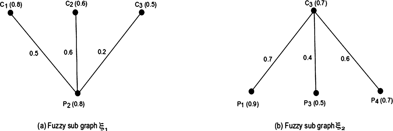
Fig. 7

Edge colouring of the fuzzy sub graphs.

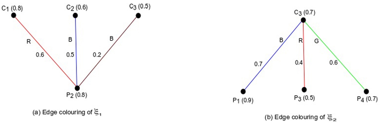
Fig. 8

CCTV for collection of data.

7Representation of Traffic Light Problem

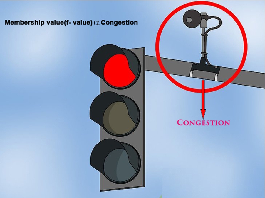
One of the most useful real life applications of the edge colouring is in traffic light problems. Traffic light system uses three standard colours: red, amber (yellow), green, following the universal colour code. The green light allows traffic to proceed in the denoted direction. The amber (yellow) light warns that more precautions should be taken to cross the road. The red signal prohibits any traffic from proceeding. However, in the present traffic light system, a traveller does not know how much the traffic is congested. This limitation has to be removed here. Traffic light system will be modified by the edge colouring of fuzzy graphs.

It takes every route as a fuzzy vertex. An edge between two vertices is drawn if the routes have a junction. The edge membership values are calculated based on the congestion of routes and the road condition. The data is collected from real time CCTV (see Fig. 8).

Thus a fuzzy graph ξ=(V,σ,μ)[TeX:] $\xi =(V,\sigma ,\mu )$ is formed. Let C=(c1,c2,…,ck)[TeX:] $C=({c_{1}},{c_{2}},\dots ,{c_{k}})$ be a set of basic colours. As traffic light system can not be used by more than three colors, the technique of the colouring is changed. In this particular traffic light system, if the colour of any edge is (ci,f(ci))[TeX:] $({c_{i}},f({c_{i}}))$, then ci[TeX:] ${c_{i}}$ is a basic colour and f(ci)[TeX:] $f({c_{i}})$ is its membership value which is calculated as f(ci)=μ(u,v)[TeX:] $f({c_{i}})=\mu (u,v)$, where μ(u,v)[TeX:] $\mu (u,v)$ is the membership value of the edge (u,v)[TeX:] $(u,v)$.

Now, a seven point crossing (for example, Park circus seven point crossing, Kolkata, West Bengal, India, see Fig. 9) is taken as an example. The image is collected from Google Maps. This picture is converted into a fuzzy graph (see Fig. 10). Now, the membership value of the edges in the figure PA, PB, PC, PD, PE, PF, AB, AF, AE, AD, AC, BC, BD, BE, BF, CD, CE, CF, DE, DF, EF are calculated from real time CCTV showing the road conjunction and the road condition. A traveller from P road can visit any route of this crossing if all routes are open at that time. So a fuzzy subgraph can be constructed against the node P to represent the travellers possible visit, whose edges are PA, PB, PC, PD, PE, PF (see Fig. 11).

Fig. 9

Seven point crossing park circus, Kolkata (collected from Google Map).

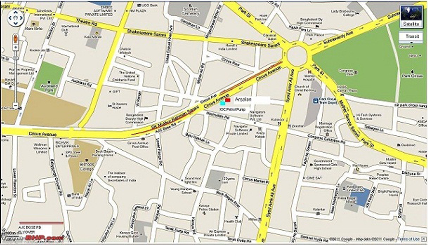
Fig. 10

Fuzzy graph of seven point crossing.

Fig. 11

Fuzzy subgraph of Fig. 10.

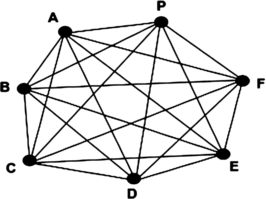
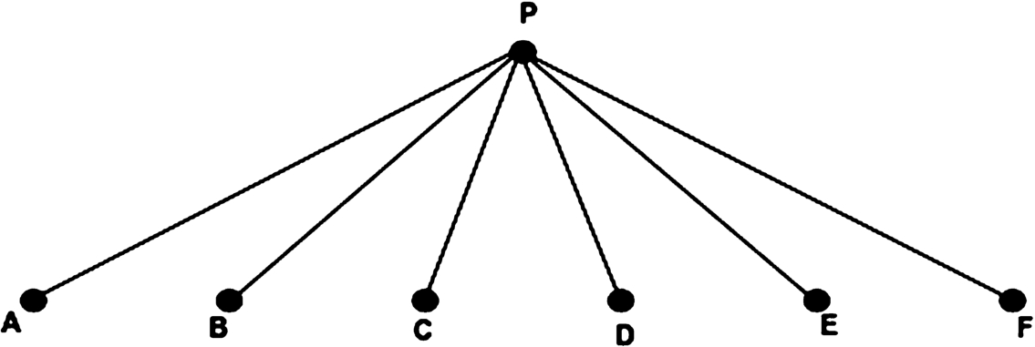
Fig. 12

Edge colouring of fuzzy graph.

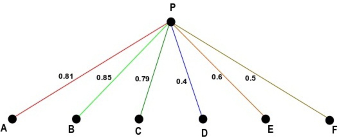
Let us consider at a particular time the membership value of the edges PA, PB, PC, PD, PE, PF be 0.81,0.85,0.79,0.4,0.6,0.5[TeX:] $0.81,0.85,0.79,0.4,0.6,0.5$, respectively. Next, this fuzzy subgraph is coloured using the edge colouring technique (see Fig. 12). In this subgraph, the chromatic index is 6 and the weight is (0.81+0.85+0.79+0.4+0.6+0.5)=3.95[TeX:] $(0.81+0.85+0.79+0.4+0.6+0.5)=3.95$.

When a traveller is travelling the P road, it would be helpful, if all the information about the next crossing was displayed in two or three display boards before the crossing. From the chromatic index the traveller can understand how many roads are open at the time of crossing, and from the weight, the total traffic condition. For this purpose, the congestion of the next crossing is to be represented in terms of percentage. Here, f-value, i.e. 0.81 indicates that the congestion is 81%[TeX:] $81\% $. Displaying percentage is helpful in order to understand the congestion of a target road. So with the help of the colouring of the fuzzy subgraph, the traveller would get an idea before crossing about the present condition of the target road. With the help of the chromatic index, the traveller also understands the situation of the target road, i.e. whether the road will open or close.

Fig. 13

Red signal with percentage of mixing of colours.

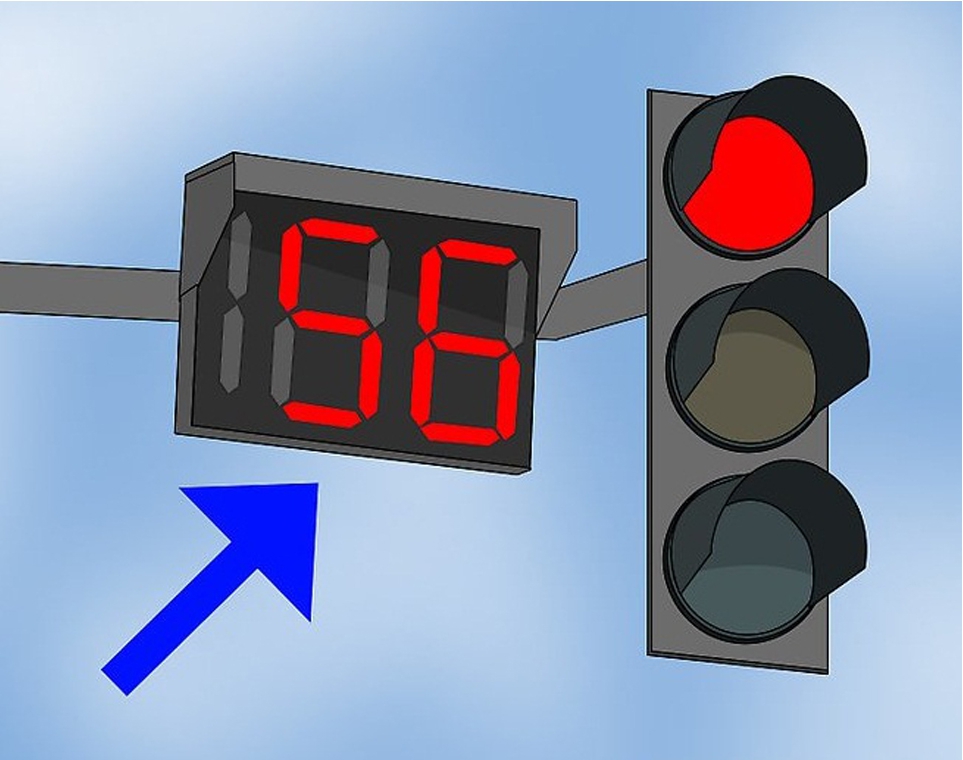
Also we can use this depth of colour in red (f(ci)[TeX:] $f({c_{i}})$) signal with percentage (see Fig. 13). If the membership value is increased, then the density of the red signal will be increased. On the other hand, the green signal can be used with the membership value 1−f1(ci)[TeX:] $1-{f^{1}}({c_{i}})$ which is the complement of the depth of red colour. The denser the green colour is, the less congested the route is. So the traveller can understand how much danger there is or how much time will be spent to cross.

The stopping time can be fixed with the help of the membership value of the red signal. If the membership value of the red colour is increased, then the stopping time will decrease.

8Conclusion

In this study, a concept of edge colouring has been introduced. A related term, chromatic index, is also defined in a different way. A weight is associated with each of the chromatic indexes. This weight might be defined in different ways. But the proposed method mentions the depth of the colours to be used to colour a graph. At the end of this paper, the traffic light problem is updated. In that problem, if the subgraph is uploaded for online traffic condition, then the input graph will be compatible with Google Traffic indicating system. It is seen that Google Traffic system calculates the data from the flow of mobiles. But here, membership values are calculated from real-time CCTV. Google Traffic uses three or four colours to represent the condition of the traffic, but the proposed method uses the colour density with a percentage, which is much more helpful to the traveller. Thus, a user can easily understand the present condition of the traffic. There are many real field problems which can be solved using this technique of colouring, such as transportation problems, social networking problems, sport modelling. The proposed method may be implemented empirically in the existing traffic light systems. The theoretical approach of edge colouring will be beneficial to other graph colouring problems as well. In future studies, more uncertainty may be represented through generalized fuzzy graphs.

References

1 | Bershtein, L.S., Bozhenuk, A.V. ((2001) ). Fuzzy coloring for fuzzy graphs. In: lEEE International Fuzzy Systems Conference, pp. 1101–1103. |
2 | Chen, L., Peng, J., Zhang, B., Li, S. ((2017) ). Uncertain programming model for uncertain minimum weight vertex covering problem. Journal of Intelligent Manufacturing, 28: (3), 625–632. |
3 | Kauffman, A. ((1973) ). Introduction a la Theorie des Sous-emsembles Flous. Masson et Cie Editeurs, Paris. |
4 | Kishore, A., Sunitha, M.S. ((2014) ). Strong chromatic number of fuzzy graphs. Annals of Pure and Applied Mathematics, 7: , 52–60. |
5 | Kishore, A., Sunitha, M.S. ((2016) ). On Injective Coloring of Graphs and Chromaticity of Fuzzy Graphs. LAP Lambert Academic Publishing. |
6 | Mahapatra, R., Samanta, S., Pal, M., Qin, X. ((2019) a). RSM index: a new way of link prediction in social networks. Journal of Intelligent and Fuzzy Systems, 37: , 2137–2151. https://doi.org/10.3233/JIFS-181452. |
7 | Mahapatra, R., Samanta, S., Allahviranloo, T., Pal, M. ((2019) b). Radio fuzzy graphs and assignment of frequency in radio stations. Computational and Applied Mathematics. https://doi.org/10.1007/s40314-019-0888-3. |
8 | Mordeson, J.N., Nair, P.S. ((2000) ). Fuzzy Graphs and Hypergraphs. Physica Verlag. |
9 | Munoz, S., Ortuno M, T., Ramirez, J., Yanez, J. ((2005) ). Coloring fuzzy graphs. Omega, 33: (3), 211–221. |
10 | Rosenfeld, A. ((1975) ). Fuzzy graphs. In: Zadeh, L.A., Fu, K.S., Shimura, M. (Eds.), Fuzzy Sets and Their Applications. Academic Press, New York, pp. 77–95. |
11 | Rosyida, I., Widodo, Indrati, C.R., Ariyanti, K., ((2015) ). A new approach in determining fuzzy chromatic index of a fuzzy graph. Journal of Intelligent and Fuzzy Systems, 28: (5), 2331–2341. |
12 | Rosyida, I., Peng, J., Chen, L., Widodo, I.C.R., Sugeng, K.A. ((2016) ). An uncertain chromatic index of an uncertain graph based on alpha-cut coloring. Fuzzy Optimization and Decision Making. https://doi.org/10.1007/s10700-016-9260-x. |
13 | Samanta, S., Pal, M. ((2013) ). Fuzzy k-competition graphs and p-competition fuzzy graphs. Fuzzy Engineering and Information, 5: (2), 191–204. |
14 | Samanta, S., Pal, M. ((2015) ). Fuzzy planar graphs. IEEE Transaction on Fuzzy Systems, 23: (6), 1936–1942. |
15 | Samanta, S., Sarkar, B., Shin, D., Pal, M. ((2016) a). Completeness and regularity of generalized fuzzy graphs. Springer Plus. https://doi.org/10.1186/s40064-016-3558-6. |
16 | Samanta, S., Pramanik, T., Pal, M. ((2016) b). Colouring of fuzzy graphs. Afrika Matematica, 27: , 37–50. |
17 | Sarkar, B., Samanta, S. ((2017) ). Generalized fuzzy trees. International Journal of Computational Intelligence Systems, 10: , 711–720. |