
A Goal Programming Model for BWM
Abstract
The best-worst method (BWM) is a multi-criteria decision-making method which works based on a pairwise comparison system. Using such a systematic pairwise comparison enhances consistency and reliability of results. The BWM results in single solution when there are two or three criteria, and for problems with fully-consistent systems, with any number of criteria. To obtain the weights of criteria for not fully-consistent comparison systems with more than three criteria, there may be a multiple optimal solution. Although multiple optimality may be desirable in some cases, in other cases, decision-makers prefer to have a unique optimal solution. This study proposes new models which result in a unique solution. The proposed models have less constraints in comparison with the previous models.
1Introduction
In recent years, multi-criteria decision-making (MCDM) methods have been developed by many researchers and applied to many real-world problems (Keshavarz-Ghorabaee et al., 2018). The MCDM can be classified into multi-attribute decision-making (MADM) and multi-objective decision-making (MODM); the MADM is for evaluation, and the MODM is for design. In the MADM, alternatives are predefined. However, the MODM designs the best alternative by considering various constraints (Hwang and Yoon, 2012).
In the past decades, several MADM methods have been proposed and the most popular methods are Best-Worst Method (BWM) (Rezaei, 2015), Analytic Hierarchy Process (AHP) (Saaty, 1986), Technique for Order of Preference by Similarity to Ideal Solution (TOPSIS) (Hwang and Yoon, 1981), ELimination and Choice Expressing REality (ELECTRE) (Roy, 1990), VIseKriterijumska Optimizacija I Kompromisno Resenje (VIKOR) (Opricovic and Tzeng, 2004), and Evaluation based on Distance from Average Solution (EDAS) (Keshavarz Ghorabaee et al., 2015).
In decision-making processes, many elements should be considered simultaneously. Therefore, it is very important to have an appropriate approach to obtain unambiguous results. There are many examples in which pairwise comparison (PC) method can be used to draw the final result in a relatively easy way (Koczkodaj, 1993). Psychologists believe that comparing two items at a time is easier and more accurate than comparing all items simultaneously (Ishizaka and Labib, 2011). The first documented use of PC returns to Ramon Llull, a 13th-century mystic and philosopher (Koczkodaj et al. 2016, 81). Condorcet (1785), Fechner (1860) and Thurstone (1927) also used PC in their studies. However, MADM is one of the most famous fields that has used PC to rank criteria or alternatives (Bozóki et al., 2016) and Saaty (1977; 1980) made the greatest impact in the popularization of the PC method by proposing Analytic Hierarchy Process (AHP) (Koczkodaj, 1993). The PC methods decompose problems into sub-problems and let experts discriminate between two items at a time. Consequently, problems can be solved easily (Brunelli and Fedrizzi, 2015). Using the PC is useful as it compels the decision maker to think about and analyse the situation more precisely and deeply (Kurttila et al., 2000). Since the comparison of two items is the simplest type of question for measuring the weights, using the PC has become an interesting topic to researchers (Kim et al., 2017).
BWM (Rezaei, 2015) is a MADM method which works based on a PC system. The most important advantages of the BWM are as follows: (1) it needs less PCs; (2) it leads to more consistency. Therefore, BWM presents more reliable results. In this method, the decision-maker identifies the best (most desirable) and the worst (least desirable) criteria. Then PCs should be obtained between each of these criteria (the best and worst) and the other criteria (Rezaei, 2015). So far, the BWM has been used in some studies (Rezaei et al., 2016, 2015; Salimi and Rezaei, 2016, 2018; Ren et al., 2017; Gupta et al., 2017; Rezaei et al., 2018). Rezaei (2016) proposed interval analysis for the case of multiple optimal solutions for not-fully consistent comparison systems and when the problem contains more than three criteria. He also proposed a linear model of the BWM. The major difference between the BWM and other PC-based methods is that those methods use the PCM (Eq. (1)) whereas the BWM uses pairwise comparison vectors (PCVs) (Eq. (2)).
(1)
(2)
Recently, the use of some PC-based methods has gained more interest, because it is possible to compute the consistency ratio, which boosts the reliability of results. However, researchers have faced difficulties in using PCMs due to rank reversal and great number of comparisons, as well as the inappropriate consistency ratio in big PCMs. The BWM was proposed by Rezaei (2015) to provide an accurate PC system with less comparisons. In addition to the possibility to compute the consistency ratio, the BWM decreases the number of comparisons to
So far, some researchers attempted to develop BWM in fuzzy environment. Guo and Zhao (2017) extended BWM to fuzzy environment and compared it with BWM. Lo and Liou (2018) proposed a hybrid model for failure mode and effect analysis. This study modifies the model of BWM according to the FBWM which was provided by Guo and Zhao (2017); they applied the interval numbers with BWM to obtain risk priority numbers. Mou et al. (2016) proposed intuitionistic fuzzy multiplicative BWM (IFMBWM) with intuitionistic fuzzy multiplicative preference relations for group decision-making. Hafezalkotob and Hafezalkotob (2017) proposed a method based on group and individual decisions supported on FBWM called GI-FBWM. The study considered a hierarchical decision framework and both democratic and autocratic decision making styles can be considered in the proposed method. Liu et al. (2018a) proposed a two-stage model for supplier selection of green fresh product. In this study, FBWM is applied for subjective criteria weights and Shannon entropy is applied for objective criteria weights. Finally, suppliers are ranked using fuzzy MULTIMOORA method. Aboutorab et al. (2018) combined the concept of Z-numbers with BWM and applied the proposed method in a supplier development problem.
Some researchers attempted to develop BWM base on rough numbers and some researchers applied rough BWM in their studies. Zavadskas et al. (2018) developed a rough SWARA approach and compared the obtained result with rough BWM and rough AHP to determine the weight values. The results showed the correlation of ranks using rough SWARA with the ranks of rough BWM and rough AHP was complete. Stević et al. (2017) proposed an approach based on rough BWM (RBWM) and rough SAW (RSAW) methods and applied the hybrid model to select wagons for internal transport of a logistics company. This study compares the obtained ranks using RBWM-RSAW with the obtained ranks using AHP-TOPSIS, AHP-MABAC, AHP-SAW, BWM-TOPSIS, BWM-MABAC, BWM-SAW, RAHP-RTOPSIS, RAHP-RSAW, RAHP-RMABAC, RBWM-RTOPSIS and RBWM-RMABAC. The results indicate that there is a high correlation between the ranks of the compared models. Stević et al. (2018) proposed an integrated model based on Rough BWM and Rough WASPAS methods. The model was applied to a location selection problem for the construction of roundabout. Through the sensitivity analysis the proposed model was compared with RBWM-RSAW, RBWM-RMABAC, RBWM-RVIKOR, RBWM-RMAIRCA, RBWM-RTOPSIS and RBWM-REDAS. The sensitivity analysis indicated that the model stability was verified. Liu et al. (2018b) combined rough number, the BWM and the VIKOR to solve a Supply chain partner selection problem under cloud computing environment. Pamučar et al. (2018) developed an approach based on interval-valued fuzzy-rough numbers (IVFRN). In this study, BWM and MABAC methods were combined and applied to evaluate firefighting aircraft. Through the sensitivity analysis, the proposed model was compared with the fuzzy and rough extension of the MABAC, COPRAS and VIKOR methods and showed a high degree of stability.
Several studies combined BWM and other MADM methods. Tian et al. (2018) combined the BWM and improved TOPSIS and developed a hybrid multi-criteria group decision-making (MCGDM) model in a green supplier selection problem. You et al. (2016) proposed a hybrid decision framework to solve MCGDM problems based on the BWM and ELECTRE III methods. Yadav et al. (2018) proposed a hybrid BWM-ELECTRE-based framework for effective offshore outsourcing adoption. In this study, having determined the weight values of offshore outsourcing enablers by employing BWM, the automotive case organizations were prioritized using ELECTRE approach. Amoozad Mahdiraji et al. (2018) applied the combination of interval BWM and fuzzy COPRAS to analyse key factors of environmental sustainability in Iranian contemporary architecture.
Keršuliene et al. (2010) developed Step-wise weight assessment ratio analysis (SWARA) to determine the weight values of the attributes. Although BWM and SWARA use different mathematical approaches, they are similar in some aspects. Identifying the best and the worst criterion in the BWM method is similar to the first step of the SWARA method. BWM and SWARA methods are more preferable than the AHP method which requires more PCs (Zolfani and Chatterjee, 2019). Zolfani et al. (2018) extended the classic SWARA method to improve the quality of decision making process. In this study, the reliability evaluation of experts’ opinion is incorporated into SWARA method. Zolfani and Chatterjee (2019) compared the results of variability between the criteria priorities for SWARA and BWM in the sustainable housing material selection problem.
Apart from the aforementioned studies, other methods are proposed to determine the weight of the attributes. Zavadskas and Podvezko (2016) proposed the Integrated Determination of Objective Criteria Weights (IDOCRIW) method to combine the weights yielded by the entropy and the Criterion Impact Loss (CILOS) methods to obtain aggregate criteria weights for objective evaluation of the data array structure. Vinogradova et al. (2018) proposed a method of weights’ recalculation, and the integration of various estimates into a single one.
Kocak et al. (2018) developed a quadratic model of Euclidean BWM and minimized the sum of the squared differences instead of maximum number of differences in BWM. However, the proposed model needs more computations in comparison with linear BWM.
The BWM provides an appropriate system to reflect DM preferences in final weights. However, for not fully-consistent comparison systems with more than three criteria, there may be multiple optimal solutions. Although multiple optimality may be desirable in some cases, in other cases, decision-makers prefer to have a unique solution. This research proposes new models which result in a unique solution. As the proposed model has less constraints in comparison with the previous models, we can mention that it involves less calculations. In Sections 2– 4, an overview of previous models is provided. In Section 5, we propose two models of the BWM. After that, a numerical example is presented in Section 6. Finally, Section 7 discusses the research conclusions.
2Best-Worst Method (BWM)
In this section, steps of the BWM to derive the weights of criteria are described. Readers can refer to Rezaei (2015) for more details.
Step 1. Determining a set of decision criteria;
Step 2. Determining the best (e.g. most desirable, most important) and the worst (e.g. least desirable, least important) criteria;
Step 3. Determining the preferences of the best criteria over all the other criteria; the Best-to-Others vector would be:
Step 4. Determining the preferences of all the criteria over the worst criteria; the Others-to-Worst vector would be:
Step 5. Solving the model and obtaining the optimal criteria weight; according to Eq. (3), we should find a solution where maximum difference between
(3)
The above model can be transformed to the following model Eq. (4).
(4)
One of the crucial features of the BWM is its ability to determine the consistency ratio. In the real world, it is not often possible to have full consistency and subjective evaluation with a high level of accuracy (Fülp et al., 2010). The existence of consistency alone can not show the level of expertise. However, the existence of inconsistency means lack of expertise or necessary information (Brunelli and Fedrizzi, 2015; Forman and Selly, 2000). The consistency ratio is calculated by Eq. (5) and the consistency index is presented in Table 1.
(5)
Table 1
Consistency table.
|
| 1 | 2 | 3 | 4 | 5 | 6 | 7 | 8 | 9 |
| Consistency index (
| 0.00 | 0.44 | 1.00 | 1.63 | 2.30 | 3.00 | 3.73 | 4.47 | 5.23 |
3Interval Weights
In the case of multi-optimality, ranges of weights can be determined. Solving Eqs. (6) and (7) for all the criteria, lower and upper bounds of the weight of each criterion can be calculated and interval weights can be obtained. The center of the interval can be used to rank the criteria or alternatives (Rezaei, 2016).
(6)
(7)
4Linear Model
The linear model of the BWM is proposed by Rezaei (2016) as in Eq. (9). In this model, instead of minimizing the maximum of
(8)
The above model can be transformed to the following linear model (Eq. (9)).
(9)
Eq. (9) is a linear model which has a unique solution. In this model,
5Proposed Models
As previously mentioned, the BWM model for not fully-consistent comparison systems with more than three criteria may result in multi-optimality solutions. It means that solving the problem results in different sets of weights for the criteria. This feature of the BWM model can be desirable in some cases. For instance, when debating is important in the decision-making process, DMs may prefer to have more information. Although multiple optimality may be desirable in some cases, in other cases, DMs prefer to have a unique solution.
In this section, we propose two models which guarantee a unique optimal solution. The proposed models use free variables (
We can mention that the number of constraints in the proposed models has significantly decreased.
5.1Proposing a Nonlinear Model
In the proposed nonlinear model, if
(10)
The consistency ratio can be also obtained by Eqs. (11) and (12). Table 1 presented by Rezaei (2015) can be used to obtain the consistency index in Eq. (8).
(11)
(12)
5.2Proposing a Linear Model
In the proposed linear model, if
(13)
The consistency ratio can be also obtained by Eqs. (11) and (12).
6Illustrative Example
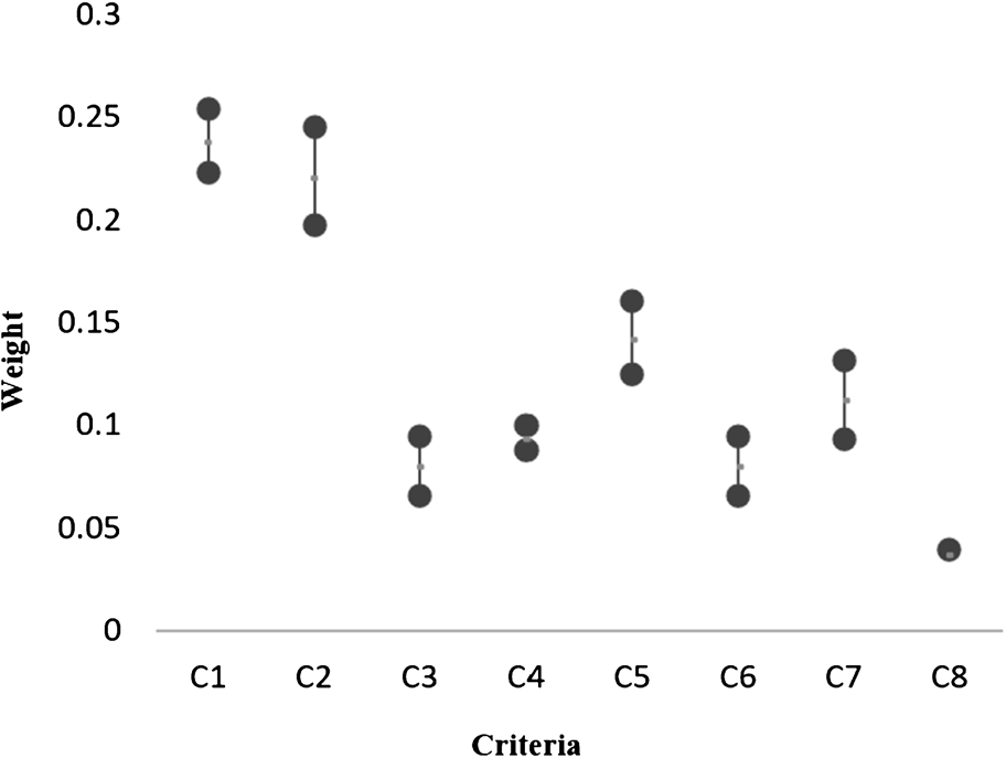
When buying a car, a customer considers eight criteria including quality
Table 2
Best-to-others (BO) and others-to-worst (OW) pairwise comparison vectors.
| BO |
|
|
|
|
|
|
|
|
| Best criterion:
| 1 | 1 | 3 | 3 | 2 | 3 | 2 | 6 |
| OW | Worst criterion:
| |||||||
|
| 6 | |||||||
|
| 6 | |||||||
|
| 2 | |||||||
|
| 3 | |||||||
|
| 4 | |||||||
|
| 2 | |||||||
|
| 3 | |||||||
|
| 1 | |||||||
According to Table 2, both
Solving this example through Eq. (4) yields
Fig. 1.
Optimal interval weights.
In some cases, DMs prefer to have a unique solution. This study proposes two models which result in a unique solution. Table 3 presents the results of application of the previous models and the proposed models to the example.
Table 3
Comparison of results of different models applied to the same data set.
| Criterion | BWM | Linear BWM | Proposed nonlinear model | Proposed linear model |
|
| 0.2318 | 0.2308 | 0.2308 | 0.2400 |
|
| 0.1994 | 0.2308 | 0.2308 | 0.2400 |
|
| 0.0882 | 0.0839 | 0.0769 | 0.0800 |
|
| 0.0912 | 0.0839 | 0.0769 | 0.0800 |
|
| 0.1411 | 0.1259 | 0.1538 | 0.1200 |
|
| 0.0882 | 0.0839 | 0.0769 | 0.0800 |
|
| 0.1241 | 0.1259 | 0.1154 | 0.1200 |
|
| 0.0359 | 0.0350 | 0.0385 | 0.0400 |
According to Table 2,
Except in the aforementioned issue, generally, Table 3 shows that the weights of criteria in all models are very close to each other. Table 4 also presents the distance from the centre of intervals which is 0.0612 for the BWM, 0.0668 for the linear BWM, 0.0559 for the proposed nonlinear model, and 0.0680 for the proposed linear model. According to the results, the solutions found by all the models are very close to the centre of intervals.
Table 4
Distances from the centre.
| Criterion | Distance | |||
| BWM | Linear BWM | Proposed nonlinear model | Proposed linear model | |
|
| 0.0064 | 0.0074 | 0.0074 | 0.0018 |
|
| 0.0217 | 0.0097 | 0.0097 | 0.0189 |
|
| 0.0082 | 0.0039 | 0.0031 | 0.0001 |
|
| 0.0025 | 0.0098 | 0.0168 | 0.0137 |
|
| 0.0016 | 0.0168 | 0.0112 | 0.0227 |
|
| 0.0082 | 0.0039 | 0.0031 | 0.0001 |
|
| 0.0117 | 0.0135 | 0.0030 | 0.0076 |
|
| 0.0010 | 0.0019 | 0.0016 | 0.0031 |
| Sum | 0.0612 | 0.0668 | 0.0559 | 0.0680 |
To compare the proposed models with the existing models, the deviation of priority ratio from initial judgment can be calculated by sum of squared errors (SSE), as defined in Eq. (14) (Mohtashami, 2014). According to Table 5, it is clear that the SSE value for the proposed nonlinear model (1.2547) is smaller than for the other models. Therefore, the proposed nonlinear model is superior to the existing models. The SSE value for the proposed linear model is also smaller than for the linear BWM. Thus, according to the results, we can conclude that the proposed models have a high level of accuracy.
(14)
7Conclusion
Table 5
SSE values for different models.
| BWM | Linear BWM | Proposed nonlinear model | Proposed linear model | |
|
| 1.9076 | 2.1459 | 1.2547 | 2 |
This research proposes novel models for BWM to generate a unique solution. For this purpose, having reviewed existing models, novel models are proposed. A numerical example is presented and differences between the previous models and proposed models are discussed. The results show that the previous models and proposed models both provide very close outcomes; however, in cases when there is more than one best (worst) item, we suggest to use the proposed models. The main advantage of applying the proposed models is that we need only
Acknowledgements
We would like to thank Dr. Jafar Rezaei for his useful comments that improved the manuscript.
References
1 | Aboutorab, H., Saberi, M., Asadabadi, M.R., Hussain, O., Chang, E. ((2018) ). ZBWM: the Z-number extension of Best Worst Method and its application for supplier development. Expert Systems with Applications, 107: , 115–125. |
2 | Amoozad Mahdiraji, H., Arzaghi, S., Stauskis, G., Zavadskas, E. ((2018) ). A hybrid fuzzy BWM-COPRAS method for analyzing key factors of sustainable architecture. Sustainability, 10: (5), 16–26. |
3 | Bozóki, S., Csató, L., Temesi, J. ((2016) ). An application of incomplete pairwise comparison matrices for ranking top tennis players. European Journal of Operational Research, 248: , 211–218. |
4 | Brunelli, M., Fedrizzi, M. ((2015) ). Boundary properties of the inconsistency of pairwise comparisons in group decisions. European Journal of Operational Research, 240: (3), 765–773. |
5 | Condorcet, M.D. ((1785) ). Essay on the Application of Analysis to the Probability of Majority Decisions. Imprimerie Royale, Paris. |
6 | Fechner, G. ((1860) ). Elements of Psychophysics. Holt, Rinehart & Wilson, New York. Translation H. Adler. |
7 | Forman, E., Selly, M.A. ((2000) ). Decision by Objectives. George Washington University. Expert Choice Inc. |
8 | Fülp, J., Koczkodaj, W.W., Szarek, S.J. ((2010) ). A different perspective on a scale for pairwise comparisons. In: Transactions on Computational Collective Intelligence I. Springer, Berlin, Heidelberg, pp. 71–84. |
9 | Guo, S., Zhao, H. ((2017) ). Fuzzy best-worst multi-criteria decision-making method and its applications. Knowledge-Based Systems, 121: , 23–31. |
10 | Gupta, P., Anand, S., Gupta, H. ((2017) ). Developing a roadmap to overcome barriers to energy efficiency in buildings using best worst method. Sustainable Cities and Society, 31: , 244–259. |
11 | Hafezalkotob, A., Hafezalkotob, A. ((2017) ). A novel approach for combination of individual and group decisions based on fuzzy best-worst method. Applied Soft Computing, 59: , 316–325. |
12 | Hwang, C.L., Yoon, K. ((1981) ). Multiple Attribute Decision Making: Methods and Applications. Springer, New York. |
13 | Hwang, C.L., Yoon, K. ((2012) ). Multiple Attribute Decision Making: Methods and Applications a State-of-the-Art Survey, (Vol. 186: ). Springer Science & Business Media. |
14 | Ishizaka, A., Labib, A. ((2011) ). Review of the main developments in the analytic hierarchy process. Expert Systems with Applications, 38: (11), 14336–14345. |
15 | Keršuliene, V., Zavadskas, E.K., Turskis, Z. ((2010) ). Selection of rational dispute resolution method by applying new step–wise weight assessment ratio analysis (SWARA). Journal of Business Economics and Management, 11: (2), 243–258. |
16 | Keshavarz Ghorabaee, M., Zavadskas, E.K., Olfat, L., Turskis, Z. ((2015) ). Multi-criteria inventory classification using a new method of evaluation based on distance from average solution (EDAS). Informatica, 26: (3), 435–451. |
17 | Keshavarz-Ghorabaee, M., Amiri, M., Zavadskas, E.K., Turskis, Z., Antucheviciene, J. ((2018) ). Simultaneous Evaluation of Criteria and Alternatives (SECA) for multi-criteria decision-making. Informatica, 29: (2), 265–280. |
18 | Kim, Y., Kim, W., Shim, K. ((2017) ). Latent ranking analysis using pairwise comparisons in crowdsourcing platforms. Information Systems, 65: , 7–21. |
19 | Kocak, H., Caglar, A., Oztas, G.Z. ((2018) ). Euclidean best–worst method and its application. International Journal of Information Technology & Decision Making, 17: (5), 1587–1605. |
20 | Koczkodaj, W.W. ((1993) ). A new definition of consistency of pairwise comparisons. Mathematical and Computer Modelling, 18: (7), 79–84. |
21 | Koczkodaj, W.W., Szybowski, J., Wajch, E. ((2016) ). Inconsistency indicator maps on groups for pairwise comparisons. International Journal of Approximate Reasoning, 69: , 81–90. |
22 | Kurttila, M., Pesonen, M., Kangas, J., Kajanus, M. ((2000) ). Utilizing the analytic hierarchy process (AHP) in SWOT analysis—a hybrid method and its application to a forest-certification case. Forest Policy and Economics, 1: (1), 41–52. |
23 | Liu, A., Xiao, Y., Ji, X., Wang, K., Tsai, S.B., Lu, H., Cheng, J., Lai, X., Wang, J. ((2018) a). A novel two-stage integrated model for supplier selection of green fresh product. Sustainability, 10: (7), 2371. |
24 | Liu, S., Hu, Y., Zhang, Y. ((2018) b). Supply chain partner selection under cloud computing environment: an improved approach based on BWM and VIKOR. Mathematical Problems in Engineering. |
25 | Lo, H.W., Liou, J.J. ((2018) ). A novel multiple-criteria decision-making-based FMEA model for risk assessment. Applied Soft Computing, 73: , 684–696. |
26 | Mohtashami, A. ((2014) ). A novel meta-heuristic based method for deriving priorities from fuzzy pairwise comparison judgments. Applied Soft Computing, 23: , 530–545. |
27 | Mou, Q., Xu, Z., Liao, H. ((2016) ). An intuitionistic fuzzy multiplicative best-worst method for multi-criteria group decision making. Information Sciences, 374: , 224–239. |
28 | Opricovic, S., Tzeng, G.H. ((2004) ). Compromise solution by MCDM methods: a comparative analysis of VIKOR and TOPSIS. European Journal of Operational Research, 156: (2), 445–455. |
29 | Pamučar, D., Petrović, I., Ćirović, G. ((2018) ). Modification of the best–worst and mabac methods: a novel approach based on interval-valued fuzzy-rough numbers. Expert Systems with Applications, 91: , 89–106. |
30 | Ren, J., Liang, H., Chan, F.T. ((2017) ). Urban sewage sludge, sustainability, and transition for Eco-City: Multi-criteria sustainability assessment of technologies based on best-worst method. Technological Forecasting and Social Change, 116: , 29–39. |
31 | Rezaei, J. ((2015) ). Best-worst multi-criteria decision-making method. Omega, 53: , 49–57. |
32 | Rezaei, J. ((2016) ). Best-worst multi-criteria decision-making method: Some properties and a linear model. Omega, 64: , 126–130. |
33 | Rezaei, J., Wang, J., Tavasszy, L. ((2015) ). Linking supplier development to supplier segmentation using best worst method. Expert Systems with Applications, 42: (23), 9152–9164. |
34 | Rezaei, J., Nispeling, T., Sarkis, J., Tavasszy, L. ((2016) ). A supplier selection life cycle approach integrating traditional and environmental criteria using the best worst method. Journal of Cleaner Production, 135: , 577–588. |
35 | Rezaei, J., Kothadiya, O., Tavasszy, L., Kroesen, M. ((2018) ). Quality assessment of airline baggage handling systems using SERVQUAL and BWM. Tourism Management, 66: , 85–93. |
36 | Roy, B. (1990). The outranking approach and the foundations of ELECTRE methods. Readings in Multiple Criteria Decision Aid, pp. 155–183. |
37 | Saaty, T.L. ((1977) ). A scaling method for priorities in hierarchical structures. Journal of Mathematical Psychology, 15: (3), 234–281. |
38 | Saaty, T.L. ((1980) ). The Analytic Hierarchy Process. McGraw-Hill, New York. |
39 | Saaty, T.L. ((1986) ). Axiomatic foundation of the analytic hierarchy process. Management Science, 32: (7), 841–855. |
40 | Salimi, N., Rezaei, J. ((2016) ). Measuring efficiency of university-industry Ph.D. projects using best worst method. Scientometrics, 109: (3), 1911–1938. |
41 | Salimi, N., Rezaei, J. ((2018) ). Evaluating firms’ R&D performance using best worst method. Evaluation and Program Planning, 66: , 147–155. |
42 | Stević, Ž., Pamučar, D., Kazimieras Zavadskas, E., Ćirović, G., Prentkovskis, O. ((2017) ). The selection of wagons for the internal transport of a logistics company: a novel approach based on rough BWM and rough SAW methods. Symmetry, 9: (11), 264. |
43 | Stević, Ž., Pamučar, D., Subotić, M., Antuchevičiene, J., Zavadskas, E. ((2018) ). The location selection for roundabout construction using Rough BWM-Rough WASPAS approach based on a new Rough Hamy aggregator. Sustainability, 10: (8), 2817. |
44 | Thurstone, L.L. ((1927) ). A law of comparative judgment. Psychological Review, 34: (4), 273–286. |
45 | Tian, Z.P., Zhang, H.Y., Wang, J.Q., Wang, T.L. ((2018) ). Green supplier selection using improved TOPSIS and best-worst method under intuitionistic fuzzy environment. Informatica, 29: (4), 773–800. |
46 | Vinogradova, I., Podvezko, V., Zavadskas, E. ((2018) ). The recalculation of the weights of criteria in MCDM methods using the bayes approach. Symmetry, 10: (6), 205. |
47 | Yadav, G., Mangla, S.K., Luthra, S., Jakhar, S. ((2018) ). Hybrid BWM-ELECTRE-based decision framework for effective offshore outsourcing adoption: a case study. International Journal of Production Research, 56: (18), 6259–6278. |
48 | You, X., Chen, T., Yang, Q. ((2016) ). Approach to multi-criteria group decision-making problems based on the best-worst-method and electre method. Symmetry, 8: (9), 95. |
49 | Zavadskas, E.K., Podvezko, V. ((2016) ). Integrated determination of objective criteria weights in MCDM. International Journal of Information Technology & Decision Making, 15: (2), 267–283. |
50 | Zavadskas, E.K., Stević, Ž., Tanackov, I., Prentkovskis, O. ((2018) ). A novel multicriteria approach–rough step-wise weight assessment ratio analysis method (R-SWARA) and its application in logistics. Studies in Informatics and Control, 27: (1), 97–106. |
51 | Zolfani, S.H., Chatterjee, P. ((2019) ). Comparative evaluation of sustainable design based on Step-Wise Weight Assessment Ratio Analysis (SWARA) and Best Worst Method (BWM) methods: a perspective on household furnishing materials. Symmetry, 11: (1), 74. |
52 | Zolfani, S.H., Yazdani, M., Zavadskas, E.K. ((2018) ). An extended stepwise weight assessment ratio analysis (SWARA) method for improving criteria prioritization process. Soft Computing, 22: (22), 7399–7405. |


