
Selection of the Most Appropriate Renewable Energy Alternatives by Using a Novel Interval-Valued Neutrosophic ELECTRE I Method
Abstract
Today energy demand in the world cannot be met based on the growing population of the countries. Exhaustible resources are not enough to supply this energy requirement. Furthermore, the pollution created by these sources is one of the most important issues for all living things. In this context, clean and sustainable energy alternatives need to be considered. In this study, a novel interval-valued neutrosophic (IVN) ELECTRE I method is conducted to select renewable energy alternative for a municipality. A new division operation and deneutrosophication method for interval-valued neutrosophic sets is proposed. A sensitivity analysis is also implemented to check the validity of the proposed method. The obtained results and the sensitivity analysis demonstrate that the given decision in the application is robust. The results of the proposed method determine that the wind power plant is the best alternative and our proposed method’s decisions are consistent and reliable through the results of comparative and sensitivity analyses.
1Introduction
Selection of the most appropriate alternative of renewable energy source is one of the most important key principles for a sustainable and clean environment. This selection process focuses to choose the best location for an anticipated purpose. Since the use of exhaustible resources in cities and industries cause air pollution, safety risks, and greenhouse gas emissions in the atmosphere, the building of a renewable energy plant becomes a more important issue for a sustainable city than ever. Furthermore, renewable energy alternative selection problem involves many criteria such as operational, environmental, social, and economic, and each of them addresses the problem in a broader and different perspective.
In multi-criteria decision making (MCDM) problems, the most important problem is the way of handling uncertainty (Mardani et al., 2015a, 2015b, 2017, 2018). In this type of problems, the criteria can be tangible or intangible. Having more intangible criteria than tangible criteria causes a harder evaluation process for experts. In this environment, MCDM methods need to determine the evaluation criteria, a set of possible alternatives, and collect the appropriate information about alternatives with respect to criteria, and to evaluate them for the decision makers’ purposes (Tzeng and Huang, 2011). To handle these difficulties, many models have been proposed and among these models, Analytic Hierarchy Process (AHP) (Saaty, 1980), Analytic Network Process (ANP) (Saaty, 1996), Technique for Order of Preference by Similarity to Ideal Solution (TOPSIS) (Hwang and Yoon, 1981; Zavadskas et al., 2016), ELimination Et Choix Traduisant la REalité (ELECTRE) (Roy, 1991; Govindan and Jepsen, 2016), VIKOR (Opricovic, 1998; Mardani et al., 2016), linguistic models (Cabrerizo et al., 2017, 2018; Morente-Molinera et al., 2019; Zhang et al., 2018; Liu et al., 2018) are the most used ones.
When considering real life conditions, things are not often precise, and they cannot be described by crisp or deterministic models. Thus, the capacity of making precise statements is quite challenging. In order to handle these vague and imprecise events, Zadeh (1965) introduced fuzzy sets together with degrees of membership of elements to these sets (Zadeh, 1965). Since that time, ordinary fuzzy sets have been extended to type-2, intuitionistic, hesitant, orthopair fuzzy sets, and neutrosophic sets. Zadeh introduced type-2 fuzzy sets to define the uncertainty of membership functions to reduce vagueness (Zadeh, 1975). Then, (Zadeh, 1975; Grattan-Guiness, 1975; Jahn, 1975; Sambuc, 1975) introduced interval-valued fuzzy sets (IVFSs), independently from each other. Atanassov introduced intuitionistic fuzzy sets (IFSs) to express decision maker’s opinions more freely by using not only membership functions but also non-membership functions of the elements in a fuzzy set (Atanassov, 1986). Hesitant fuzzy sets (HFSs) were introduced by Torra (2010) in order to operate with a set of possible membership values for an element in a fuzzy set (Torra, 2010). Despite all these extensions, fuzzy sets could not handle all types of uncertainties such as indeterminate and inconsistent information.
In order to tackle this inadequacy, Smarandache (1995) introduced neutrosophic logic and neutrosophic sets (Smarandache, 1999). A neutrosophic set is composed of three subsets which are degree of truthiness
The first ELECTRE method, ELECTRE I, was introduced by Roy (1968). The roots of its development are based on the construction of a contradictory and very heterogeneous set of criteria, and quantitative and qualitative consequences which are not only associated with numerical ordinal scales but also are attached with imprecise, uncertain, and ill-determined knowledge of data (Roy, 1968). The other types of ELECTRE methods are ELECTRE IS, ELECTRE II, ELECTRE III, ELECTRE IV, and ELECTRE TRI. These methods mainly hold ELECTRE I characteristics and link to its basic idea. Briefly, ELECTRE I and ELECTRE IS are introduced for the selection problems; ELECTRE TRI, for the assignment problems, and ELECTRE II, III and IV, for the ranking problems (Leyva López, 2005). Since our problem’s characteristics hold heterogeneous and multi-criteria structure; qualitive and quantitative consequences build on interval-number scales; uncertain and indeterminate knowledge, it is proper to apply ELECTRE I method.
In this study, an IVN ELECTRE I method is developed and applied to a renewable energy sources alternative selection for a county municipality. The originality of this paper can be explained with 3 basics. Firstly, we develop a novel interval-valued neutrosophic ELECTRE I method and apply it to a renewable energy source selection. Secondly, a new and an efficient deneutrosophication and division operation is proposed. Finally, for validating the proposed method, we compare the results with the interval-valued neutrosophic (IVN) TOPSIS method. A sensitivity analysis with an explanatory pattern is also performed to demonstrate the stability of the ranking results of the IVN ELECTRE I method. We believe that our study can guide the researchers who are interested in decision making under imprecise and indeterminate environment.
The remainder of this paper is prepared as follows. Section 2 reviews the literature related to the neutrosophic MCDM. In Section 3, renewable energy source alternatives and criteria are determined. In Section 4, preliminaries for IVN neutrosophic sets are given. In Section 5, an application for a county municipality to determine the best renewable energy source is introduced by using the proposed IVN ELECTRE I method. The paper ends with the conclusions and suggestions for further research.
2Literature Review: Neutrosophic MCDM Methods
Neutrosophic sets have been used in several single and multiple decision-making methods in recent years. The number of studies on neutrosophic sets and its applications has increased dramatically since 2010. The types of neutrosophic sets in the literature are singleton, interval-valued, triangular, or trapezoidal neutrosophic sets. These studies have been briefly summarized in the following.
Bausys et al. (2015) applied neutrosophic sets to COPRAS method for the decision making problems by using uncertain data. Sun et al. (2015) extended Choquet integral operator with interval neutrosophic numbers for multi-criteria decision making problems. Bausys and Zavadskas (2015) extended VIKOR method with interval valued neutrosophic sets for the multi-criteria decision making problems. Zavadskas et al. (2015) applied WASPAS method with single-valued neutrosophic set for the assessment of locations for the construction site of a waste incineration plant. Ye (2016b) introduced correlation coefficients of interval neutrosophic hesitant fuzzy sets for the MCDM problems. Li et al. (2016) introduced Some single valued neutrosophic number heronian mean operators for the MCDM problems. Ye studied the cross-entropy of single valued neutrosophic sets (SVNSs) as an extension of the cross entropy of fuzzy sets. The practical example showed the effectiveness of the proposed cross entropy method for MCDM techniques (Ye, 2014). Ye developed a multiple attribute group decision-making method by using the neutrosophic linguistic numbers weighted arithmetic average (NLNWAA) and neutrosophic linguistic numbers weighted geometric average (NLNWGA) operators (Ye, 2016a). Ma et al. studied a problem of time-aware trustworthy service selection which is formulated as MCDM problem of creating ranked services list using cloud service interval neutrosophic set (CINS) (Ma et al., 2016). It was solved by developing a CINS ranking method. The developed model which is based on a real-world dataset shows the practicality and effectiveness of the proposed approach. Huang defined a new distance measure between two SVNSs (Huang, 2016). The study figured out that neutrosophic sets are very effective to define incompleteness, indeterminacy and inconsistency information. Baušys and Juodagalvienė studied a location selection problem of the garage at the parcel of a single-family residential house by using an integrated method of AHP and Weighted Aggregated Sum-Product Assessment (WASPAS) with SVNSs (Baušys and Juodagalvienė, 2017). They reveal that the application of SVNSs allows to model uncertainty of the initial information clearly. Peng et al. presented an MCDM problem based on the Qualitative Flexible Multiple Criteria (QUALIFLEX) method where the criteria values are addressed by multi-valued neutrosophic information (Peng et al., 2017a). Stanujkic et al. (2017) extended MULTIMOORA method to single valued neutrosophic sets. Zavadskas et al. (2017) applied single-valued neutrosophic MAMVA method for the sustainable market evaluation of buildings. The assessments showed that the given decisions by the proposed method are robust and can be applied to various application areas. Akram & Sitara studied an SVN graph structure which is a generalization of fuzzy graph structures (Akram and Sitara, 2017). Applications of SVN graph structures in decision-making problems showed that using neutrosophic sets allow to clarify uncertainty of the complex environments. The illustrative example of choosing the best manufacturing alternative in the flexible manufacturing system indicated the robustness of the proposed methodologies. Şahin presented prioritized aggregation operators for aggregating the normal neutrosophic information and then extended these operators to the generalized prioritized weighted aggregation operators (Şahin, 2017). The results of the study indicated that normal neutrosophic sets are a powerful tool for handling incompleteness, indeterminacy, and inconsistency of evaluation information. Ye (2017) introduced weighted aggregation operators of trapezoidal neutrosophic numbers for the MCDM problems. Liang et al. (2017) applied single-valued trapezoidal neutrosophic DEMATEL method for the evaluation of e-commerce websites. Zhang et al. proposed a restaurant decision support model using social information for tourists on TripAdvisor.com by using interval-valued neutrosophic numbers (Zhang et al., 2017). The paper found out that the new model considers the active, neutral and passive information in online reviews all at once and takes the inter-dependency among criteria into consideration on tourists’ decision-making. Peng et al. presented a new outranking approach for MCDM problems, which are developed in the context of a simplified neutrosophic environment by singleton subsets in
In this paper, unlike the above papers, an interval-valued neutrosophic ELECTRE I is presented for alternative energy source selection problem of a county municipality. Since evaluation criteria include not only uncertain but also incomplete, indeterminate and inconsistent characteristics in the evaluation process, interval-valued neutrosophic sets are used to handle this handicap. In the literature, multi-valued neutrosophic ELECTRE III and single valued neutrosophic ELECTRE methods have been developed by Peng et al. (2016, 2014), Feng et al. (2018). The models in Peng et al. (2016) and (2014) are based on single valued neutrosophic sets and do not present a flexible definition area for T, I, F values to decision makers. Feng et al. (2018) developed an interval valued neutrosophic ELECTRE III method for the shopping mall photovoltaic plan selection. However, our proposed method includes novel deneutrosophication and division operators together with comprehensive linguistic scales in order to weigh the criteria and to assess the alternatives. In this paper, we develop ELECTRE I method by using interval-valued neutrosophic sets to a new deneutrosophication method and a new division operator for interval-valued neutrosophic sets. We believe this paper can guide researchers to the application of interval-valued neutrosophic sets to other MCDM techniques.
3Neutrosophic Sets: Preliminaries
Smarandache introduced neutrosophic sets as an extension of intuitionistic fuzzy sets. They have become very popular in recent years and have been used in many MCDM methods such as neutrosophic AHP (Radwan et al., 2016); neutrosophic TOPSIS (Chi and Liu, 2013; Nădăban and Dzitac, 2016); neutrosophic EDAS (Peng and Liu, 2017).
Definition 1.
Let X be a universe of discourse. A single-valued neutrosophic set A in X is:
(1)
Definition 2.
Let X be a universe of discourse. An IVN set N in X is independently characterized by the intervals
(2)
Let
1.
2.
3.
4.
5.
Definition 3.
Let
Definition 4.
Let
(3)
There are few deneutrosophication methods for comparing neutrosophic numbers (Zhang et al., 2015; Biswas et al., 2016). We propose a new deneutrosophication method in order to compare the interval-valued neutrosophic numbers. It is given in Definition 5.
Definition 5.
Let
(4)
4Proposed Methodology
IVN ELECTRE I method’s steps are given as follows:
Step 1: Construct the IVN decision matrices (
Table 1
Scale of IVN decision matrix.
| Linguistic term | ||
| CB | Certainly bad | |
| VB | Very bad | |
| B | Bad | |
| BA | Below average | |
| F | Fair | |
| AA | Above average | |
| G | Good | |
| VG | Very good | |
| CG | Certainly good | |
The illustrated decision matrix (DM) based on Expert j opinions is presented in Table 2.
Step 2: Aggregate the DMs to obtain aggregated IVN decision matrix
Table 2
DM based on expert j opinions.
| Criterion | Type | … | |||
| Linguistic cost | |||||
| Numerical cost | |||||
| ⋮ | ⋮ | ⋮ | ⋮ | ⋱ | ⋮ |
| Linguistic Benefit | ... |
Step 3: Calculate the weighted normalized DM (R).
Table 3
Aggregated DM.
| Criterion | Type | … | |||
| Linguistic cost | |||||
| Numerical cost | |||||
| ⋮ | ⋮ | ⋮ | ⋮ | ⋱ | ⋮ |
| Linguistic benefit | ... |
Normalization of formulas for benefit (
(5)
(6)
Arithmetic operations are carried out with the neutrosophic formulas given in Definition 2, and Definition 3. After calculations, normalized IVN DM
Table 4
Normalized decision matrix.
| Criterion | Type | … | |||
| Linguistic cost | |||||
| Numerical cost | |||||
| ⋮ | ⋮ | ⋮ | ⋮ | ⋱ | ⋮ |
| Linguistic benefit | ... |
Table 5
Scale for criteria weighting (Karaşan and Kahraman, 2017).
| Linguistic term | ||
| TI | Trivial importance | |
| UII | Unimportant importance | |
| USI | Unsatisfied importance | |
| LF | Lower than fair | |
| FI | Fair importance | |
| MF | More than fair | |
| SI | Satisfied importance | |
| II | Impactful importance | |
| CII | Certainly impactful importance | |
Weighted normalized IVN DM (V) is obtained by multiplying the IVN weights vector (
(7)
Table 6 presents the weighted normalized IVN DM.
Step 4: Obtain the Concordance and Discordance Indices.
Table 6
Weightednormalized IVN decision matrix.
| Criterion | Type | … | |||
| Linguistic cost | |||||
| Numerical cost | |||||
| ⋮ | ⋮ | ⋮ | ⋮ | ⋱ | ⋮ |
| Linguistic benefit | ... |
Let A
Concordance index (
(8)
(9)
Step 5: Calculate the Concordance matrix.
The Concordance index
(10)
(11)
Step 6: Calculate the Discordance matrix.
Similarly, the Discordance index
(12)
If q and z are used to show the weighted normalized values, the discordance matrix can be given as in Eq. (13).
(13)
Step 7: Determine the threshold value for Concordance and Discordance matrices.
The threshold value for Concordance matrix
(14)
(15)
Step 8: Determine the acceptable relations based on (
The proposed extension of ELECTRE I method offers ready-made scales to decision makers in order to express their opinions efficiently. It conducts new deneutrosophication and division operators for interval-valued neutrosophic sets. Besides, our model is relatively easy to use and produces robust decisions.
5Application
Managers of a municipal which is close to sea coast want to invest in renewable energy technologies for self-meeting their energy need. Expert group indicated that they were not sure neither about the exact values of measurable criteria nor about the values of linguistic criteria since the related data depend on uncertain environmental, political, and economic conditions. Hence, we used neutrosophic sets in order to handle the uncertainty and indeterminacy caused by the mentioned conditions. Experts utilized Table 2 and Table 6 to score decision matrices. Figure 1 presents the hierarchy of the application.
Fig. 1
Hierarchy of the application.
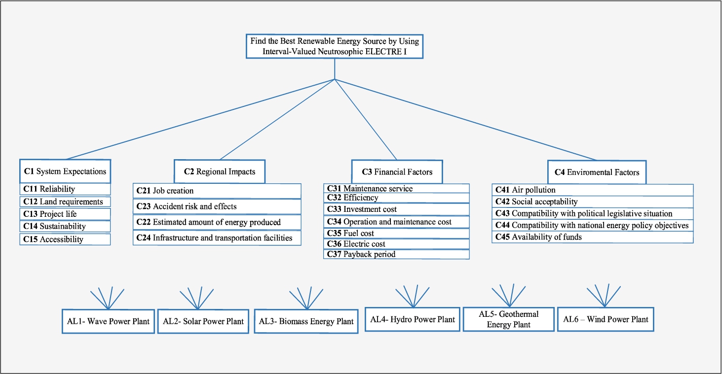
5.1Renewable Energy Alternatives and Decision Criteria
Renewable energy sources involve biomass energy, geothermal energy, ocean energy, solar energy, wind energy, and hydropower energy. They have an enormous potential to meet energy needs of the world. By doing that, the energy security of the world can be powered by modern conversion technologies by reducing the long-term price of fuels from conventional sources, and decreasing the use of fossil fuels. Using renewable energies does not only impact on reducing the air pollution, safety risks, and greenhouse gas emissions in the atmosphere but also they are recycled in nature. Furthermore, it reduces dependence on imported fuels and creates new jobs and provides regional employment. Taking into consideration the above, we firstly introduce the general characteristics of alternatives, then the selection criteria.
AL1 wave power plant: The immense energy potential of the oceans is being increasingly recognized all over the world (Hammar et al., 2017). This immense energy which is called here ’ocean wave energy’ is the conversion to the energy of wind waves by using generators which are placed on the surface of the ocean. The generated energy is usually used in desalination plants, power plants, and water pumps. The main factors that effect the rate of the energy output are determined by wave height, wave speed, wave length, water density, and temperature (Khan et al., 2017).
AL2 solar power plant: Solar energy is simply an energy source provided by the sun in the form of solar radiation. It is also called photovoltaic energy which means conversion of light into electricity. Starting with the first use, it dates back to the year the 1870s, and this technology is pollution and often noise free. In order to establish a solar energy system, there are some basic criteria to evaluate, such as requirements and properties of installation area, accessibility to that area, the infrastructure of the transmission of the generated electricity, governmental funds for the investment (Onar et al., 2015; Çelikbilek and Tüysüz, 2016).
AL3 biomass energy plant: Biomass energy is widely available, naturally distributed and, most importantly, converts waste into energy that helps to deal with pollution. Four main types of biomass, wood plants and herbaceous plants and grasses are the main types of interest for producing energy, with attention focused on the crops corn or maize, sugarcane, sorghum, and millets, as well as the switchgrass which has been utilized as a source of biofuel (McKendry, 2002; Cebi et al., 2016)]. It has been used as an energy source from the 1800s. Since that time, several characteristics affect the performance of biomass fuel such as the heat value, moisture level, compositions, and size.
AL4 hydro power plant: Hydropower is power derived from the energy of falling water or fast running water. Hydropower plants are used to transform the kinematic energy of falling water to the electricity. A turbine converts the kinetic energy of falling water into mechanical energy. Then a generator uses the mechanical energy generated by the turbine for producing electrical energy. In order to establish a hydropower energy system, there are some basic criteria to evaluate such as efficiency, costs, environmental effects, governmental funds.
AL5 geothermal energy plant: Geothermal energy is produced from the heat generated by Earth’s formation, and subsequent radioactive decay of the earth’s minerals (Wang et al., 2017). Geothermal energy relies on heat from Earth to generate steam and produce electricity. The utilization of geothermal energy depends on the demand for heat or electricity and the distance of the resource from the end consumer, resource temperature, and chemistry of the geothermal fluid (Amoo, 2014).
AL6 wind power plant: Wind energy is a carbon-free energy source depending on average wind speeds, wind turbine hubs, and turbulence intensity. There is a tendency of the use of wind energy that increased rapidly since the 1970s, starting with the oil embargo crisis. Since that time, it is possible to construct a wind energy system depending on country policies, supply chain issues of transmission and integration with the electricity system, compatibility of social and environmental conditions to the investment, economic concerns, regional deployment.
Various criteria for the evaluation of renewable energy alternatives have been used by several researchers (Onar et al., 2015; Çelikbilek and Tüysüz, 2016; Kahraman et al., 2010a, 2010b, 2009; Kaya and Kahraman, 2010; Şengül et al., 2015; Büyüközkan and Güleryüz, 2016; Diemuodeke et al., 2016; Väisänen et al., 2016; Quan and Leephakpreeda, 2015). After analysing these studies, the most common criteria have been listed and sorted for the proposed IVN ELECTRE I method. The evaluation criteria for renewable energy alternatives that will be used in this study are given in Table 7.
Table 7
Evaluation criteria for renewable energy alternatives.
| Main criteria | Sub criteria |
| C1 system expectations | C11 Reliability |
| C12 Land requirements | |
| C13 Project life | |
| C14 Sustainability | |
| C15 Accessibility | |
| C2 regional impacts | C21 Job creation |
| C22 Estimated amount of energy produced | |
| C23 Accident risk and effects | |
| C24 Infrastructure and transportation facilities | |
| C3 financial factors | C31 Maintenance service |
| C32 Efficiency | |
| C33 Investment cost | |
| C34 Operation and maintenance cost | |
| C35 Fuel cost | |
| C36 Electric cost | |
| C37 Payback period | |
| C4 environmental factors | C41 Air pollution |
| C42 Social acceptability | |
| C43 Compatibility with political legislative situation | |
| C44 Compatibility with national energy policy objectives | |
| C45 Availability of funds |
5.2Problem Solution
Table 8 presents the linguistic evaluations for the sub-criteria collected from the experts. These evaluations are aggregated to obtain the weights of the sub-criteria.
Table 8
Linguistic evaluations of sub-criteria with respect to experts.
| Sub-criteria | DM1 | DM2 | DM3 | |
| C11 | Reliability | II | SI | II |
| C12 | Land requirements | LF | FI | FI |
| C13 | Project life | LF | USI | UII |
| C14 | Sustainability | II | TI | USI |
| C15 | Accessibility | LF | USI | TI |
| C21 | Job creation | LF | USI | USI |
| C22 | Estimated amount of energy produced | SI | II | SI |
| C23 | Accident risk and effects | TI | TI | USI |
| C24 | Infrastructure and transportation facilities | USI | USI | TI |
| C31 | Maintenance service | USI | USI | TI |
| C32 | Efficiency | USI | TI | USI |
| C33 | Investment cost | SI | SI | SI |
| C34 | Operation and maintenance cost | SI | SI | MF |
| C35 | Fuel cost | MF | SI | MF |
| C36 | Electric cost | MF | SI | FI |
| C37 | Payback period | MF | MF | FI |
| C41 | Air pollution | MF | FI | FI |
| C42 | Social acceptability | TI | UII | UII |
| C43 | Compatibility with political legislative situation | LF | FI | LF |
| C44 | Compatibility with national energy policy objectives | LF | USI | LF |
| C45 | Availability of funds | CII | II | II |
The aggregated weights of the sub-criteria results as interval-valued neutrosophic sets are given in Table 9.
Table 9
Aggregated weighting results of the sub-criteria.
| Criterion | Aggregated results | Criterion | Aggregated results |
| C11 | C33 | ||
| C12 | C34 | ||
| C13 | C35 | ||
| C14 | C36 | ||
| C15 | C37 | ||
| C21 | C41 | ||
| C22 | C42 | ||
| C23 | C43 | ||
| C31 | C44 | ||
| C32 | C45 |
After the calculation of criteria which is needed for weighted normalized IVN decision matrix and concordance interval matrix in the later parts, we construct the decision matrices with respect to experts. To indicate the types of criteria, C-N, C-L, B-L, and B-N are used as Cost-Numerical, Cost-Linguistic, Benefit-Linguistic, and Benefit-Numerical for short. Experts weights are 0.4 for academicians, and 0.3, for the managers from the energy sector. Table 10 illustrates the linguistic terms which are revealed by these experts.
Table 10
DM based on expert opinions.
| Criterion | Type | E1 | E2 | E3 | |||||||||||||||
| AL1 | AL2 | AL3 | AL4 | AL5 | AL6 | AL1 | AL2 | AL3 | AL4 | AL5 | AL6 | AL1 | AL2 | AL3 | AL4 | AL5 | AL6 | ||
| C11 | B-N | G | AA | BA | B | VB | G | G | BA | AA | AA | F | G | CB | B | BA | F | BA | CG |
| C12 | C-N | BA | AA | CG | G | AA | F | BA | AA | G | VG | CG | AA | BA | B | VB | B | BA | F |
| C13 | B-N | AA | G | BA | AA | G | BA | AA | G | VG | F | AA | BA | BA | AA | BA | VG | G | CG |
| C14 | B-L | AA | F | AA | G | VG | B | AA | VB | B | B | BA | CG | AA | F | BA | B | B | VB |
| C15 | B-N | AA | F | AA | VB | B | B | AA | F | BA | F | AA | BA | AA | F | BA | VG | G | CG |
| C21 | B-N | AA | G | AA | F | BA | G | F | G | BA | VG | B | VB | AA | G | BA | F | VB | G |
| C22 | B-N | G | BA | G | B | B | AA | AA | G | BA | VG | B | B | G | BA | F | AA | AA | AA |
| C23 | C-L | BA | BA | VG | B | B | G | F | BA | F | CG | G | G | AA | BA | AA | AA | AA | G |
| C24 | C-L | VG | F | CG | G | G | E | VB | CB | B | BA | F | CB | CG | A | CG | B | B | A |
| C31 | C-L | B | B | BA | F | CB | G | B | BA | B | VB | AA | CG | B | BA | B | AA | AA | G |
| C32 | B-L | AA | B | VB | AA | CG | AA | AA | BA | AA | BA | BA | AA | AA | VG | G | CG | BA | AA |
| C33 | C-N | CG | AA | BA | BA | AA | BA | CG | BA | CG | B | B | BA | CG | B | B | VB | B | BA |
| C34 | C-N | AA | BA | AA | AA | AA | G | AA | BA | F | VB | B | G | AA | CB | VB | B | AA | G |
| C35 | C-N | BA | BA | F | VB | F | G | F | F | AA | AA | BA | G | BA | F | BA | F | F | G |
| C36 | C-N | BA | F | AA | AA | F | G | BA | F | VB | B | F | BA | F | VB | B | G | F | G |
| C37 | C-N | VG | F | VB | B | VB | BA | VG | G | CG | AA | F | BA | AA | AA | BA | G | BA | VG |
| C41 | C-N | VB | F | VB | AA | AA | G | B | B | VB | AA | F | F | VB | B | F | BA | BA | VG |
| C42 | B-L | BA | AA | G | AA | F | AA | VG | G | CG | VB | AA | G | CG | AA | F | BA | F | CG |
| C43 | B-L | B | B | G | F | AA | BA | B | B | VB | F | B | BA | VB | CB | B | F | B | BA |
| C44 | B-L | CB | VB | B | B | B | BA | CB | VB | B | G | AA | F | B | BA | B | G | B | VB |
| C45 | B-N | CB | CB | AA | B | B | BA | CB | B | VB | G | F | AA | AA | BA | AA | B | B | BA |
The next step is the aggregation of decision matrices given in linguistic terms in Table 10. Aggregated IVN DM (A) is obtained by using Eq. (3) as in Table 11.
Table 11
Aggregated DM.
| Criterion | Type | … | |||
| Linguistic cost | |||||
| Numerical cost | |||||
| ⋮ | ⋮ | ⋮ | ⋮ | ⋱ | ⋮ |
| Numerical benefit | |||||
| ⋮ | ⋮ | ⋮ | ⋮ | ⋱ | ⋮ |
| Linguistic benefit |
Table 12
Weighted normalized DM.
| Criterion | Type | … | |||
| Linguistic cost | |||||
| Numerical cost | |||||
| ⋮ | ⋮ | ⋮ | ⋮ | ⋱ | ⋮ |
| Numerical benefit | |||||
| ⋮ | ⋮ | ⋮ | ⋮ | ⋱ | ⋮ |
| Linguistic benefit |
In the next step, we obtain the weighted normalized DM (R). In Eqs. (5), (6), and (7), all operations are calculated as is given in Definition 2. In Eq. (6), number 1 is represented in interval-neutrosophic set as
In the next step, we calculate the concordance and discordance indices based on the proposed deneutrosophication method which is given in Definition 5. Due to the excessive number of pairwise comparisons, we will only present Concordance and Discordance indices of Alternative 1 in the following. Concordance indices for Alternative 1:
Table 13
Concordance matrix of deneutrosoficated IVN values.
| 0.72 | 0.51 | 0.47 | 0.23 | 0.35 | |
| 0.28 | – | 0.38 | 0.22 | 0.19 | 0.12 |
| 0.54 | 0.62 | – | 0.49 | 0.3 | 0.41 |
| 0.47 | 0.78 | 0.51 | – | 0.27 | 0.35 |
| 0.77 | 0.81 | 0.7 | 0.73 | – | 0.62 |
| 0.68 | 0.88 | 0.59 | 0.65 | 0.38 | – |
Table 14
Discordance matrix of deneutrosoficated IVN values.
| – | 0.02 | 0.16 | 0.15 | 0.8 | 0.06 |
| 0.31 | – | 0.15 | 0.13 | 0.84 | 0.08 |
| 0.05 | 0.03 | – | 0.03 | 0.77 | 0.11 |
| 0.15 | 0.04 | 0.06 | – | 0.76 | 0.13 |
| 1 | 0.69 | 0.75 | 0.69 | – | 0.7 |
| 0.3 | 0.07 | 0.22 | 0.21 | 0.77 | – |
Based on the threshold value that is calculated by using Eq. (14), the concordance index matrix is given in Table 15. The threshold value is calculated as 0.595.
Table 15
Concordance index matrix.
| – | 1 | 1 | 0 | 0 | 0 |
| 0 | – | 0 | 0 | 0 | 0 |
| 1 | 1 | – | 0 | 0 | 0 |
| 0 | 1 | 1 | – | 0 | 0 |
| 1 | 1 | 1 | 1 | – | 1 |
| 1 | 1 | 1 | 1 | 0 | – |
Table 16
Discordance index matrix.
| – | 1 | 1 | 1 | 0 | 1 |
| 1 | – | 1 | 1 | 0 | 1 |
| 1 | 1 | – | 1 | 0 | 1 |
| 1 | 1 | 1 | – | 0 | 1 |
| 0 | 0 | 0 | 0 | – | 0 |
| 1 | 1 | 1 | 1 | 0 | – |
Based on the threshold value that is calculated by using Eq. (15), the discordance index matrix is given in Table 16. The threshold value is calculated as 0.405.
The last step is the comparison of the Concordance and Discordance index matrices. In Table 15, the value 1 represents that the value of the index is equal to or larger than the threshold. In Table 16, the value 1 represents that the value of the index is smaller than the threshold. If we have the values 1 in the same cells of Tables 15 and 16, it is concluded that the row alternative is better than the column alternative. Through this matching, AL6-Wind Power Plant is determined to be the best alternative that the municipality can invest in. The outranking relations of the alternatives are given in Fig. 2.
Fig. 2
Outranking relations of the alternatives.
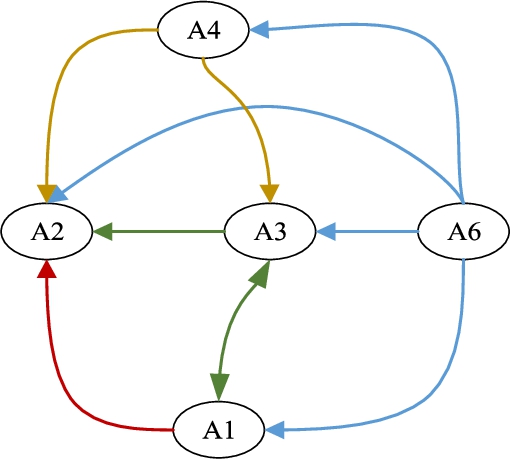
The arrows in Table 2 indicate that AL6-Wind Power Plant is the best among the alternatives, A3-Hydropower Energy Plant is the second best. A1-Wave Power Plant – A3-Biomass Energy Plant are non-comparable among themselves and A5-Geothermal Energy Plant is non-comparable among all alternatives.
5.3Comparative Analysis
In this section, the proposed IVN ELECTRE I method is compared with IVN TOPSIS method developed by Chi and Liu (2013). Since we apply the same scales which are given in Table 1 and Table 5 for IVN TOPSIS method, the results in Table 12 are used for the next steps of the IVN TOPSIS. After the calculations, positive and negative ideal solutions of IVN TOPSIS are given in Table 17.
Table 17
Positive and negative solutions of the IVN TOPSIS.
| C11 | ||
| C12 | ||
| ⋮ | ⋮ | ⋮ |
| C21 | ||
| ⋮ | ⋮ | ⋮ |
| C45 |
Distances to negative and positive ideal solutions are given in Table 18.
Table 18
Positive and negative ideal solutions of the IVN TOPSIS.
| Positive ideal solution | Negative ideal solution | |
| AL1 | ||
| AL2 | ||
| AL3 | ||
| AL4 | ||
| AL5 | ||
| AL6 |
Closeness coefficient (
5.4Sensitivity Analysis
To demonstrate the stability of the ranking results, a sensitivity analysis (SA) is performed based on the weights of criteria. We develop a pattern to determine the one-at-a-time sensitivity for every sub-criterion. The values of these criteria are every linguistic term which is given in Table 5. After the changes on weights of sub-criteria through this pattern, IVN ELECTRE I operations according to changing weights are re-run and the selection of the best alternative is re-processed. The developed pattern is given in Table 19.
Table 19
Pattern of the one-at-a-time SA.
| Based on the sub-criteria | |||||
| Solution sets | Solution sets | Solution sets | |||
| Variables | CLI | Best alternative | Best alternative | ||
| VLI | ⋮ | ⋱ | ⋮ | ||
| LI | ⋮ | ⋱ | ⋮ | ||
| BAI | ⋮ | ⋱ | ⋮ | ||
| AI | ⋮ | ⋱ | ⋮ | ||
| AAI | ⋮ | ⋱ | ⋮ | ||
| HI | ⋮ | ⋱ | ⋮ | ||
| VHI | ⋮ | ⋱ | ⋮ | ||
| CHI | Best alternative | Best alternative | |||
The final results of the SA with the determined best alternative are given in Table 20.
Table 20
Results of the one-at-the-time sensitivity analysis.
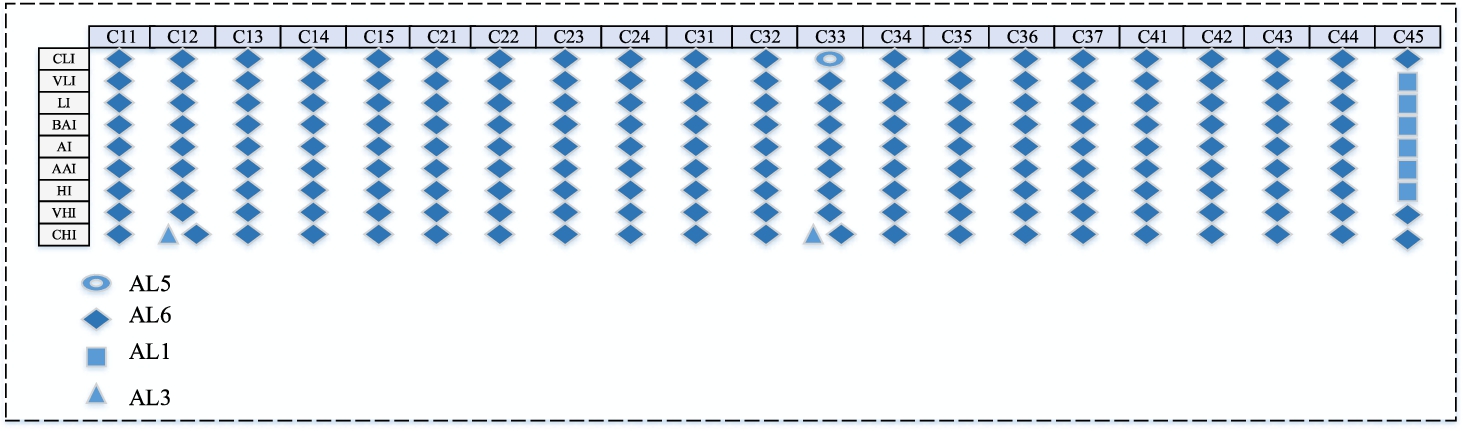
When the results are examined, it seems that the changes made on the 3 criteria which are C12-Land requirements, C33-Investment cost, and C45-Availability of funds have different solutions from the others for finding the best alternative. When the linguistic term is increased from CLI-Certainly Low Importance to CHI-Certainly High Importance for the criterion C12-Land requirements, AL3-Biomass energy plant becomes one of the best alternatives with AL-6 Wind Power Plant since biomass energy plant’s energy production volume is exactly dependent on the area that it is established. When the linguistic term is increased to linguistic term CHI-Certainly High Importance on criterion C33-Investment cost, AL3-Biomass energy plant becomes again one of the best alternatives with AL-6 Wind Power Plant. But, while the linguistic term is CLI-Certainly Low Importance, AL5-Geothermal energy plant is the best alternative. Lastly, when the linguistic term is increased to linguistic term CHI-Certainly High Importance on criterion C45-Availability of funds, AL1-Wave Power Plant becomes the best alternative since it is an area that has not been invested by the private sector enough. In all cases, AL6-Wind Power Plant is the best alternative by a majority and only in special cases that match up with real life our proposed method chooses different alternatives.
6Conclusion
In multi-criteria decision making (MCDM) problems, the most important problem is the way of handling not only the uncertainty that is the result of lack of knowledge, but also its incompleteness, indeterminacy, and inconsistency level due to the expert groups. The selection of the best renewable energy sources depends not only on alternatives and criteria but also on scoring alternatives with respect to criteria by experts. In this complex environment where the inconsistency arises, the scope of ordinary fuzzy sets is insufficient. To overcome these problems, neutrosophic logic is introduced by Smarandache. In this study, we applied neutrosophic sets to an MCDM model to overcome this impreciseness and indeterminacy in measuring the criteria numerically.
In this paper, an interval-valued neutrosophic multi-criteria group decision making with the ELECTRE method has been proposed for the selection of the most appropriate renewable energy source for a county municipality. Alternatives and criteria have been determined by experts’ ideas and literature review. The importance degrees of the criteria have been determined by aggregation of expert opinions and the scores of alternatives are provided by experts for applying them to interval-valued neutrosophic ELECTRE. In the application, 21 sub-criteria were evaluated using interval-valued neutrosophic sets. According to the obtained results from the aggregation, C45-Availability of Funds is determined as the most efficient sub-criterion. The second and third important sub-criteria are C11-Reliability and C22-Estimated Amount of Energy Produced, respectively. In the interval-valued neutrosophic ELECTRE I method, there are 3 experts who evaluated 6 alternatives with respect to 21 sub-criteria. According to the results, A6-Wave Power Plant is determined as the best alternative for the most appropriate renewable energy source for a municipality. Sensitivity analysis demonstrates that our proposed model is robust. The usage of deneutrosophication operator can be mentioned as a drawback of the proposed method since a complete neutrosophic approach should be preferred.
For further studies, proposed division operation and deneutrosophication method can be extended to singleton neutrosophic sets, triangular neutrosophic sets, or trapezoidal neutrosophic sets. The proposed interval-valued neutrosophic ELECTRE method can be applied to the other areas such as location selection, strategy assessment, construction management, etc. The proposed method can be a basis for other possible neutrosophic outranking methods such as neutrosophic PROMETHEE method and neutrosophic ORESTE method.
Compliance with Ethical Standards
Conflict of Interest: All the authors declare that they have no conflict of interest.
Ethical approval: All procedures performed in studies involving human participants were in accordance with the ethical standards of the institutional and/or national research committee and with the 1964 Helsinki declaration and its later amendments or comparable ethical standards.
Informed consent: Informed consent was obtained from all individual participants included in the study.
References
1 | Abdel-Basset, M., Mohamed, M., Smarandache, F. ((2018) ). An extension of neutrosophic AHP–SWOT analysis for strategic planning and decision-making. Symmetry, 10: (4), 116. |
2 | Akram, M., Sitara, M. ((2017) ). Novel applications of single-valued neutrosophic graph structures in decision-making. Journal of Applied Mathematics and Computing, 1–32. |
3 | Amoo, O.M. ((2014) ). Thermodynamic-based resource classification of renewable geothermal energy in Nigeria. Journal of Renewable and Sustainable Energy, 6: (3), 033129. |
4 | Atanassov, K. ((1986) ). Intuitionistic fuzzy sets. Fuzzy Sets and Systems, 20: (1), 87–96. |
5 | Baušys, R., Juodagalvienė, B. ((2017) ). Garage location selection for residential house by WASPAS-SVNS method. Journal of Civil Engineering and Management, 23: (3), 421–429. |
6 | Bausys, R., Zavadskas, E.K. ((2015) ). Multicriteria decision making approach by VIKOR under interval neutrosophic set environment. Economic Computation and Economic Cybernetics Studies and Research, 49: (4), 33–48. |
7 | Bausys, R., Zavadskas, E.K., Kaklauskas, A. ((2015) ). Application of neutrosophic set to multicriteria decision making by COPRAS. Economic Computation and Economic Cybernetics Studies and Research, 49: (1), 91–105. |
8 | Biswas, P., Pramanik, S., Giri, B.C. ((2016) ). TOPSIS method for multi-attribute group decision-making under single-valued neutrosophic environment. Neural Computing and Applications, 27: (3), 727–737. |
9 | Büyüközkan, G., Güleryüz, S. ((2016) ). An integrated DEMATEL-ANP approach for renewable energy resources selection in Turkey. International Journal of Production Economics, 182: , 435–448. |
10 | Cabrerizo, F.J., Al-Hmouz, R., Morfeq, A., Balamash, A.S., Martínez, M.A., Herrera-Viedma, E. ((2017) ). Soft consensus measures in group decision making using unbalanced fuzzy linguistic information. Soft Computing, 21: (11), 3037–3050. |
11 | Cabrerizo, F.J., Morente-Molinera, J.A., Pedrycz, W., Taghavi, A., Herrera-Viedma, E. ((2018) ). Granulating linguistic information in decision making under consensus and consistency. Expert Systems with Applications, 99: , 83–92. |
12 | Chi, P., Liu, P. ((2013) ). An extended TOPSIS method for the multiple attribute decision making problems based on interval neutrosophic set. Neutrosophic Sets and Systems, 1: (1), 63–70. |
13 | Cebi, S., Ilbahar, E., Atasoy, A. ((2016) ). A fuzzy information axiom based method to determine the optimal location for a biomass power plant: a case study in Aegean Region of Turkey. Energy, 116: , 894–907. |
14 | Çelikbilek, Y., Tüysüz, F. ((2016) ). An integrated grey based multi-criteria decision-making approach for the evaluation of renewable energy sources. Energy, 115: , 1246–1258. |
15 | Diemuodeke, E.O., Hamilton, S., Addo, A. ((2016) ). Multi-criteria assessment of hybrid renewable energy systems for Nigeria’s coastline communities. Energy, Sustainability, and Society, 6: (1), 26. |
16 | Feng, J., Li, M., Li, Y. ((2018) ). Study of Decision framework of shopping mall photovoltaic plan selection based on DEMATEL and ELECTRE III with symmetry under neutrosophic set environment. Symmetry, 10: (5), 150. |
17 | Govindan, K., Jepsen, M.B. ((2016) ). ELECTRE: a comprehensive literature review on methodologies and applications. European Journal of Operational Research, 250: (1), 1–29. |
18 | Grattan-Guiness, I. ((1975) ). Fuzzy membership mapped onto interval and many-valued quantities. Z. Math. Logik. Grundladen Math. 22. |
19 | Hammar, L., Gullström, M., Dahlgren, T.G., Asplund, M.E., Goncalves, I.B., Molander, S. ((2017) ). Introducing ocean energy industries to a busy marine environment. Renewable and Sustainable Energy Reviews, 74: , 178–185. |
20 | Huang, H.L. ((2016) ). New distance measure of single-valued neutrosophic sets and its application. International Journal of Intelligent Systems, 31: (10), 1021–1032. |
21 | Hwang, C.L., Yoon, K. ((1981) ). Multiple Criteria Decision Making. Lecture Notes in Economics and Mathematical Systems, Vol.186: . |
22 | Jahn, K. ((1975) ). Intervall-wertige Mengen. Mathematische Nachrichten, 68: , 115–132. 1975. |
23 | Ji, P., Zhang, H.Y., Wang, J.Q. ((2018) ). A projection-based TODIM method under multi-valued neutrosophic environments and its application in personnel selection. Neural Computing and Applications, 29: (1), 221–234. |
24 | Kahraman, C., Kaya, İ., Cebi, S. ((2009) ). A comparative analysis for multiattribute selection among renewable energy alternatives using fuzzy axiomatic design and fuzzy analytic hierarchy process. Energy, 34: (10), 1603–1616. |
25 | Kahraman, C., Cebi, S., Kaya, I. ((2010) a). Selection among Renewable Energy Alternatives Using Fuzzy Axiomatic Design: The Case of Turkey. Journal of Universal Computer Science, 16: (1), 82–102. |
26 | Kahraman, C., Kaya, I., Çebi, S. ((2010) b). Renewable energy system selection based on computing with words. International Journal of Computational Intelligence Systems, 3: (4), 461–473. |
27 | Karaşan, A., Kahraman, C. ((2017) ). Interval-valued neutrosophic extension of EDAS method. In: Advances in Fuzzy Logic and Technology 2017. Springer, pp. 343–357. |
28 | Kaya, T., Kahraman, C. ((2010) ). Multicriteria renewable energy planning using an integrated fuzzy VIKOR & AHP methodology: the case of Istanbul. Energy, 35: (6), 2517–2527. |
29 | Khan, N., Kalair, A., Abas, N., Haider, A. ((2017) ). Review of ocean tidal, wave and thermal energy technologies. Renewable and Sustainable Energy Reviews, 72: , 590–604. |
30 | Leyva López, J.C. ((2005) ). Multicriteria decision aid application to a student selection problem. Pesquisa Operacional, 25: (1), 45–68. |
31 | Li, Y., Liu, P., Chen, Y. ((2016) ). Some single valued neutrosophic number heronian mean operators and their application in multiple attribute group decision making. Informatica, 27: (1), 85–110. |
32 | Liang, R., Wang, J., Zhang, H. ((2017) ). Evaluation of e-commerce websites: An integrated approach under a single-valued trapezoidal neutrosophic environment. Knowledge-Based Systems, 135: , 44–59. |
33 | Liu, Y., Dong, Y., Liang, H., Chiclana, F., Herrera-Viedma, E. (2018). Multiple attribute strategic weight manipulation with minimum cost in a group decision making context with interval attribute weights information. IEEE Transactions on Systems, Man, and Cybernetics: Systems. |
34 | Ma, H., Hu, Z., Li, K., Zhang, H. ((2016) ). Toward trustworthy cloud service selection: a time-aware approach using interval neutrosophic set. Journal of Parallel and Distributed Computing, 96: , 75–94. |
35 | Mardani, A., Jusoh, A., Nor, K., Khalifah, Z., Zakwan, N., Valipour, A. ((2015) a). Multiple criteria decision-making techniques and their applications–a review of the literature from 2000 to 2014. Economic Research-Ekonomska Istraživanja, 28: (1), 516–571. |
36 | Mardani, A., Jusoh, A., Zavadskas, E.K. ((2015) b). Fuzzy multiple criteria decision-making techniques and applications–Two decades review from 1994 to 2014. Expert Systems with Applications, 42: (8), 4126–4148. |
37 | Mardani, A., Zavadskas, E., Govindan, K., Amat Senin, A., Jusoh, A. ((2016) ). VIKOR technique: a systematic review of the state of the art literature on methodologies and applications. Sustainability, 8: (1), 37. |
38 | Mardani, A., Zavadskas, E.K., Khalifah, Z., Zakuan, N., Jusoh, A., Nor, K.M., Khoshnoudi, M. ((2017) ). A review of multi-criteria decision-making applications to solve energy management problems: Two decades from 1995 to 2015. Renewable and Sustainable Energy Reviews, 71: , 216–256. |
39 | Mardani, A., Jusoh, A., Halicka, K., Ejdys, J., Magruk, A., Ahmad U. N, U. ((2018) ). Determining the utility in management by using multi-criteria decision support tools: a review. Economic Research-Ekonomska Istraživanja, 31: (1), 1666–1716. |
40 | McKendry, P. ((2002) ). Energy production from biomass (part-1): overview of biomass. Bioresource Technology, 83: (1), 37–46. |
41 | Morente-Molinera, J.A., Kou, G., Pang, C., Cabrerizo, F.J., Herrera-Viedma, E. ((2019) ). An automatic procedure to create fuzzy ontologies from users’ opinions using sentiment analysis procedures and multi-granular fuzzy linguistic modelling methods. Information Sciences, 476: , 222–238. |
42 | Nădăban, S., Dzitac, S. ((2016) ). May. Neutrosophic TOPSIS: A general view. In: 2016 6th International Conference on Computers Communications and Control (ICCCC). IEEE, pp. 250–253. |
43 | Onar, S.C., Oztaysi, B., Otay, İ., Kahraman, C. ((2015) ). Multi-expert wind energy technology selection using interval-valued intuitionistic fuzzy sets. Energy, 90: , 274–285. |
44 | Opricovic, S. ((1998) ). Multicriteria optimization of civil engineering systems. Faculty of Civil Engineering, Belgrade, 2: (1), 5–21. |
45 | Peng, X., Liu, C. (2017). Algorithms for neutrosophic soft decision making based on EDAS and new similarity measure. |
46 | Peng, J.J., Wang, J.Q., Zhang, H.Y., Chen, X.H. ((2014) ). An outranking approach for multi-criteria decision-making problems with simplified neutrosophic sets. Applied Soft Computing, 25: , 336–346. |
47 | Peng, J.J., Wang, J.Q., Wu, X.H. ((2016) ). An extension of the ELECTRE approach with multi-valued neutrosophic information. Neural Computing and Applications, 1–12. |
48 | Peng, J.J., Wang, J.Q., Yang, W.E. ((2017) a). A multi-valued neutrosophic qualitative flexible approach based on likelihood for multi-criteria decision-making problems. International Journal of Systems Science, 48: (2), 425–435. |
49 | Peng, J.J., Wang, J.Q., Tian, C., Wu, X.H., Chen, X.H. (2017b). A multi-criteria decision-making approach based on Choquet integral-based TOPSIS with simplified neutrosophic sets. |
50 | Quan, P., Leephakpreeda, T. ((2015) ). Assessment of wind energy potential for selecting wind turbines: an application to Thailand. Sustainable Energy Technologies and Assessments, 11: , 17–26. |
51 | Radwan, N., Senousy, M.B., Riad, A. ((2016) ). Neutrosophic AHP multi criteria decision making method applied on the selection of learning management system. International Journal of Advancements in Computing Technology, 8: (5), 95–105. |
52 | Rivieccio, U. ((2008) ). Neutrosophic logics: prospects and problems. Fuzzy Sets and Systems, 159: (14), 1860–1868. |
53 | Roy, B. ((1968) ). Classement et choix en présence de points de vue multiples (la méthode ELECTRE). RIRO, 8: , 57–75. |
54 | Roy, B. ((1991) ). The outranking approach and the foundations of ELECTRE methods. Theory and decision, 31: (1), 49–73. |
55 | Saaty, T.L. ((1980) ). The Analytic Hierarchy Process: Planning. Priority Setting. Resource Allocation. MacGraw-Hill, New-York International Book Company, New York. |
56 | Saaty, T.L. ((1996) ). Decision Making with Dependence and Feedback: The Analytic Network Process, Vol. 4922: . RWS Publications, Pittsburgh. |
57 | Sambuc, R. ((1975) ). Fonctions ϕ-floues. Application l’aide au diagnostic en pathologie thyroidienne. Univ. Marseille, France. |
58 | Smarandache, F. ((1999) ). A unifying field in logics: neutrosophic logic. In: Philosophy. American Research Press, pp. 1–141. |
59 | Stanujkic, D., Zavadskas, E.K., Smarandache, F., Brauers, W.K., Karabasevic, D. ((2017) ). A neutrosophic extension of the MULTIMOORA method. Informatica, 28: (1), 181–192. |
60 | Sun, H.X., Yang, H.X., Wu, J.Z., Ouyang, Y. ((2015) ). Interval neutrosophic numbers Choquet integral operator for multi-criteria decision making. Journal of Intelligent & Fuzzy Systems, 28: (6), 2443–2455. |
61 | Şahin, R. ((2017) ). Normal neutrosophic multiple attribute decision making based on generalized prioritized aggregation operators. Neural Computing and Applications, 1–21. |
62 | Şengül, Ü., Eren, M., Shiraz, S.E., Gezder, V., Şengül, A.B. ((2015) ). Fuzzy TOPSIS method for ranking renewable energy supply systems in Turkey. Renewable Energy, 75: , 617–625. |
63 | Torra, V. ((2010) ). Hesitant fuzzy sets. International Journal of Intelligent Systems, 25: , 529–539. 2010. |
64 | Tzeng, G., Huang, J. ((2011) ). Multiple Attribute Decision Making Methods and Applications. CRC Press, Taylor and Francis Group, A Chapman & Hall Book, Boca Raton. |
65 | Väisänen, S., Mikkilä, M., Havukainen, J., Sokka, L., Luoranen, M., Horttanainen, M. ((2016) ). Using a multi-method approach for decision-making about a sustainable local distributed energy system: a case study from Finland. Journal of Cleaner Production, 137: , 1330–1338. |
66 | Wang, H., Smarandache, F., Zhang, Y., Sunderraman, R. ((2005) a). Single valued neutrosophic sets. In: Proceedings of 10th 476 International Conference on Fuzzy Theory and Technology, Salt Lake City, p. 477. |
67 | Wang, H., Smarandache, F., Zhang, Y.Q., Sunderraman, R. ((2005) b). Interval Neutrosophic Sets and Logic: Theory and Applications in Computing. Hexis, Phoenix. |
68 | Wang, X., Gao, Q., Jiang, Y., Bai, L. ((2017) ). Analysis on thermal behavior of the type of filter tubes of extraction-injection wells in geothermal utilization. Applied Thermal Engineering, 118: , 233–243. |
69 | Ye, J. ((2014) ). Single valued neutrosophic cross-entropy for multicriteria decision making problems. Applied Mathematical Modelling, 38: (3), 1170–1175. |
70 | Ye, J. ((2016) a). Aggregation operators of neutrosophic linguistic numbers for multiple attribute group decision making. SpringerPlus, 5: (1), 1691. |
71 | Ye, J. ((2016) b). Correlation coefficients of interval neutrosophic hesitant fuzzy sets and its application in a multiple attribute decision making method. Informatica, 27: (1), 179–202. |
72 | Ye, J. ((2017) ). Some weighted aggregation operators of trapezoidal neutrosophic numbers and their multiple attribute decision making method. Informatica, 28: (2), 387–402. |
73 | Zadeh, L. ((1965) ). Fuzzy sets. Information and Control, 8: , 338–353. 1965. |
74 | Zadeh, L. ((1975) ). The concept of a linguistic variable and its application to approximate reasoning-1. Information Sciences, 8: , 199–249. 1975. |
75 | Zavadskas, K.E., Baušys, R., Lazauskas, M. ((2015) ). Sustainable assessment of alternative sites for the construction of a waste incineration plant by applying WASPAS method with single-valued neutrosophic set. Sustainability, 7: (12), 15923–15936. |
76 | Zavadskas, E.K., Mardani, A., Turskis, Z., Jusoh, A., Nor, K.M. ((2016) ). Development of TOPSIS method to solve complicated decision-making problems—An overview on developments from 2000 to 2015. International Journal of Information Technology & Decision Making, 15: (03), 645–682. |
77 | Zavadskas, E.K., Bausys, R., Kaklauskas, A., Ubarte, I., Kuzminske, A., Gudiene, N. ((2017) ). Sustainable market valuation of buildings by the single-valued neutrosophic MAMVA method. Applied Soft Computing, 57: , 74–87. |
78 | Zhang, H.Y., Wang, J.Q., Chen, X.H. ((2015) ). An outranking approach for multi-criteria decision-making problems with interval valued neutrosophic sets. Neural Computing & Applications. |
79 | Zhang, H.Y., Ji, P., Wang, J.Q., Chen, X.H. ((2017) ). A novel decision support model for satisfactory restaurants utilizing social information: a case study of TripAdvisor.com. Tourism Management, 59: , 281–297. |
80 | Zhang, H., Dong, Y., Herrera-Viedma, E. ((2018) ). Consensus building for the heterogeneous large-scale GDM with the individual concerns and satisfactions. IEEE Transactions on Fuzzy Systems, 26: (2), 884–898. |


