An Adaptive Algorithm for Calculating Crosstalk Error for Blind Source Separation

1Introduction

Blind signal separation (BSS) technology originated from the famous “cocktail party” problem (Choi and Cichocki, 1997) and has been a key research issue since then (Bridwell et al., 2018; Yatabe and Kitamura, 2018). It attempts to separate the unknown original signals only by using the observations of their mixture without having any prior information of the source signals and channels. It is important to measure the effectiveness of the blind separation algorithms, since it affects not only the effect of the algorithms, but also the iterative process of the algorithms. Evaluating the quality of the waveforms of the signals and the similarity of the waveforms is the most straightforward way to judge the effectiveness of algorithm. However, this method can only be regarded as a qualitative analysis, which cannot quantitatively reflect the stability and convergence rate of the algorithm. Therefore, researchers have proposed some performance indexes, such as crosstalk error (Cichocki and Amari, 2002; Parra and Sajda, 2003; El-Sankary et al., 2015), correlation coefficient (Li et al., 2012) and signal-to-noise ratio (Laheld and Cardoso, 1993; Li and Sejnowski, 1995; Grellier and Comon, 1998; Nandakumar and Bijoy, 2014; Aroudi et al., 2016; Mirzal, 2017) etc. The consistence between the order of the source signals and the separated signals is needed for calculating most of the performance indexes, but the order of the separated signals is uncertain. The crosstalk error does not need to consider the correspondence, and it can reflect the separation effect directly.

The crosstalk error represents the approximate degree between the global separation matrix C and a diagonal matrix. When C is closer to a diagonal matrix or its permutation matrix, the smaller the crosstalk error, the more similar the separated signals are to the source signals. Theoretically, the crosstalk error should be a good performance index in the field of BSS (Macchi, 1993; Moreau and Macchi, 1996; Amari, 1997; Yang and Amari, 1997; Moreau and Macchi, 1998; Macchi and Moreau, 1999; Yang, 1999; Basak and Amari, 1999). However, it is very sensitive to numerical errors and can not be directly used to evaluate separation effects in many practical situations. On one hand, in order to calculate the crosstalk error, it needs to know C in advance, which means that it cannot directly be applied to real-world experiments. On the other hand, if the maximum value of each row of C is in the same column, the crosstalk error usually does not correctly evaluate the separation effect. In this case, small crosstalk errors do not indicate that the separation effect is good. Since each component of the separated signal is an approximate estimation of the same source signal component, the actual separation effect is poor. The above two shortcomings affect its practical application. In order to overcome the above problems, Li Zong have proposed a method to improve crosstalk error evaluation criterion by introducing correlation coefficients to measure the degree of correlation between the separated signal components and adding them to the calculation formula of crosstalk error (Li et al., 2012). Although this method improves the accuracy of the evaluation when the maximum values of two rows of C are in the same column, C is still unknown when calculating crosstalk error in the practical application. Zhang used the Least Mean Square (LMS) algorithm to estimate C in real time (Zhang et al., 2011). However, the convergence rate of the method is limited by the convergence step size of the algorithm, and once the step size is inappropriate, the algorithm will fail. At the same time, when the value changes subtly in C (Mansour et al., 2002), the crosstalk error may vary greatly. In other words, the crosstalk error is not robust.

In response to the above problems, a fully adaptive crosstalk error estimation model based on the recursive least square (RLS) algorithm is presented in this paper. This new approach consists of sifting the impact of step size on the estimation of crosstalk error. Furthermore, the robustness of the crosstalk error is improved by introducing the position information of the maximum value of each row in the global separation matrix C in the process of calculating the crosstalk error.

The paper is organized as follows. In Section 2, the shortcomings of the original performance index are analysed. The main contributions of the paper can be found in Section 3, where the fully adaptive crosstalk error estimation model is presented firstly, and then the position information of the maximum value of each row is introduced to improve the robustness of the crosstalk error. Finally, the whole process of the algorithm is explained. The validity of the proposed algorithm is verified by experimental analysis in Section 4. Finally, Section 5 contains some conclusions.

2Problem Formulation

Suppose that an antenna array is made up of M units, therefore the instantaneous linear mixing model can be expressed as

In order to simplify the problem of BSS and reduce the computational complexity, it is generally necessary to pre-whiten the signal, and the signal after whitening is

In practice, the blind source separation algorithms can only make C as close as possible to a generalized permutation matrix. Based on this, in order to evaluate the performance of the separation algorithms, the literature (Cichocki and Amari, 2002) gave a measurement method by using the difference between C and a generalized permutation matrix, which is named as crosstalk error and expressed as

In matrices C1[TeX:] ${\mathbf{C}_{1}}$ and C2[TeX:] ${\mathbf{C}_{2}}$, the maximum value of every row is in the first column, so the isolated signal is only the same signal. The corresponding separation effect of C1[TeX:] ${\mathbf{C}_{1}}$ and C2[TeX:] ${\mathbf{C}_{2}}$ is very poor, and the value of PI(C1)[TeX:] $\mathit{PI}({\mathbf{C}_{1}})$ and PI(C2)[TeX:] $\mathit{PI}({\mathbf{C}_{2}})$ should be very big. However, the crosstalk errors of them are PI(C1)=0.00002[TeX:] $\mathit{PI}({\mathbf{C}_{1}})=0.00002$ and PI(C2)=0.00057[TeX:] $\mathit{PI}({\mathbf{C}_{2}})=0.00057$, which are very small. At the same time, from matrices PI(C1)[TeX:] $\mathit{PI}({\mathbf{C}_{1}})$ and PI(C2)[TeX:] $\mathit{PI}({\mathbf{C}_{2}})$, we can also see that the crosstalk error will change greatly even though there is a minor change in C.

Therefore, the maximum value of all the rows in the C should be in different columns. However, from the definition of formula (6), this restriction is not considered. Therefore, in this paper, we add the position information of the maximum value of each row in the C to the definition of the crosstalk error to improve the robustness of the crosstalk error.

3A New Algorithm for Calculating the Crosstalk Error

For overcoming the shortcomings of the original crosstalk error, firstly a model for estimating the mixed matrix A is established and the corresponding analytic solution is given in this section. Then, the position information constraint is introduced into the definition of crosstalk error to improve its robustness. Finally, the whole process of the algorithm for calculating the crosstalk error is given.

3.2Location Introduction

It can be seen from the first section that some isolated signals may be the same signal, if the maximum value of the corresponding rows share the same column. Therefore, an improved crosstalk error definition is proposed here to eliminate the wrong decision caused by positions of optimal values in the same column, which is defined as

(23)

PI(C)=1n(n−1){∑i=1n(∑j=1n|cij|maxk|cik|−1)+∑j=1n(∑i=1n|cij|maxk|ckj|∏p=1j(1+rp)−1)},[TeX:] \[\begin{aligned}{}\mathit{PI}(\mathbf{C})& =\frac{1}{n(n-1)}\Bigg\{{\sum \limits_{i=1}^{n}}\Bigg({\sum \limits_{j=1}^{n}}\frac{|{c_{ij}}|}{{\max _{k}}|{c_{ik}}|}-1\Bigg)\\ {} & \hspace{1em}+{\sum \limits_{j=1}^{n}}\Bigg({\sum \limits_{i=1}^{n}}\frac{|{c_{ij}}|}{{\max _{k}}|{c_{kj}}|}{\prod \limits_{p=1}^{j}}(1+{r_{p}})-1\Bigg)\Bigg\},\end{aligned}\]

where rp=1[TeX:] ${r_{p}}=1$, and rp=0[TeX:] ${r_{p}}=0$ or rp>0[TeX:] ${r_{p}}>0$, when p=2,3,…,n[TeX:] $p=2,3,\dots ,n$. Let rp>0[TeX:] ${r_{p}}>0$, if the column with the maximum value in row p is same as any other rows before row p, otherwise rp=0[TeX:] ${r_{p}}=0$, for p=2,3,…,n[TeX:] $p=2,3,\dots ,n$. rp[TeX:] ${r_{p}}$ is a factor for punishing the proximity of C to a generalized permutation matrix.

Crosstalk errors given in (6) and (23) are equal while C is a generalized permutation matrix (maximum values in every row share different columns). However, the crosstalk error increases when the global separation matrix is in the situations described in (Zhang et al., 2011). The more maximum values in different rows share the same column, the worse the effect of blind source separation is and the greater the crosstalk error calculated by equation (23) is. Thus, the proposed adaptive calculation method of the crosstalk error can evaluate the effectiveness of blind source separation algorithm. Plugging the solutions of the location optimizations into the algorithm, we get the complete adaptive algorithm for calculating the crosstalk error. The pseudo code of the proposed algorithm is given in Algorithm 1.

Algorithm 1

Pseudo code of the proposed algorithm

4Experiments and Analysis

In this section, the proposed algorithm is evaluated by two methods, which are simulation experiment and real world experiment.

4.1Simulation Experiments

The new proposed crosstalk error definition defined by formula (23) is used to recalculate the crosstalk error of the matrixes described by the formulas (7). The new crosstalk error values are PI(C1)=1.3000[TeX:] $\mathit{PI}({\mathbf{C}_{1}})=1.3000$ and PI(C2)=1.3021[TeX:] $\mathit{PI}({\mathbf{C}_{2}})=1.3021$, respectively. It can be seen that the new crosstalk error that can reflect the effectiveness of BSS is poor, and improves the instability of the crosstalk error that due to the small value changes effectively.

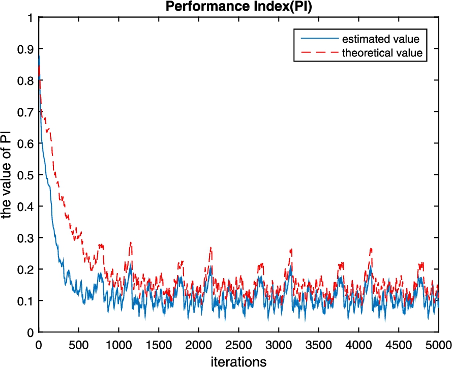
Fig. 1

Comparison of the estimation of PI[TeX:] $\mathit{PI}$ and the theoretical value of PI[TeX:] $\mathit{PI}$.

In order to verify the robustness of the new proposed calculation method for evaluating BSS, two simulation examples for comparison are presented. First, we use the natural gradient RLS algorithm mentioned in literature (Zhu and Zhang, 2002) as the BSS algorithm. The source signal vector is

St=[sign(cos(310πt)),sin(1600πt),sin(600πt+5cos(60πt)),sin(180πt)]T,[TeX:] \[ {\mathbf{S}_{t}}={\big[\operatorname{sign}(\cos (310\pi t)),\hspace{2.5pt}\sin (1600\pi t),\hspace{2.5pt}\sin (600\pi t+5\cos (60\pi t)),\hspace{2.5pt}\sin (180\pi t)\big]^{T}},\]

where the superscript T is the meaning of matrix transposition. In this experiment, the sampling rate is taken as 10 KHz. The number of sampling points is 5000. A is randomly generated by the function A=randn(4,4)[TeX:] $\mathbf{A}=\texttt{randn(4,4)}$ of MATLAB library. Let W=I[TeX:] $\mathbf{W}=\mathbf{I}$, where I is the unit matrix. Zero-mean independent Gaussian white noise is added to the mixtures, and the signal-to-noise ratio is 20 dB. The forgetting factor of the algorithm is 0.993. The proximity of the estimation of PI[TeX:] $\mathit{PI}$ calculated by our proposed algorithm and the theoretical value of PI[TeX:] $\mathit{PI}$ calculated by the conventional RLS algorithm is shown in Fig. 1, the value of the crosstalk error is the average of 500 Monte Carlo trials.

According to the initial conditions, the initial values of the estimated and theoretical values are 0.8669 and 0.8412, respectively. From Fig. 1, it is found that the difference between the estimated value and the theoretical value in the initial 500 iterations is obvious, but then the difference between them decreases with the increase of the number of iterations. Obviously, the trend of them is consistent and the estimated value of our proposed algorithm is more accurate than the theoretical value.

Fig. 2

The source signals.

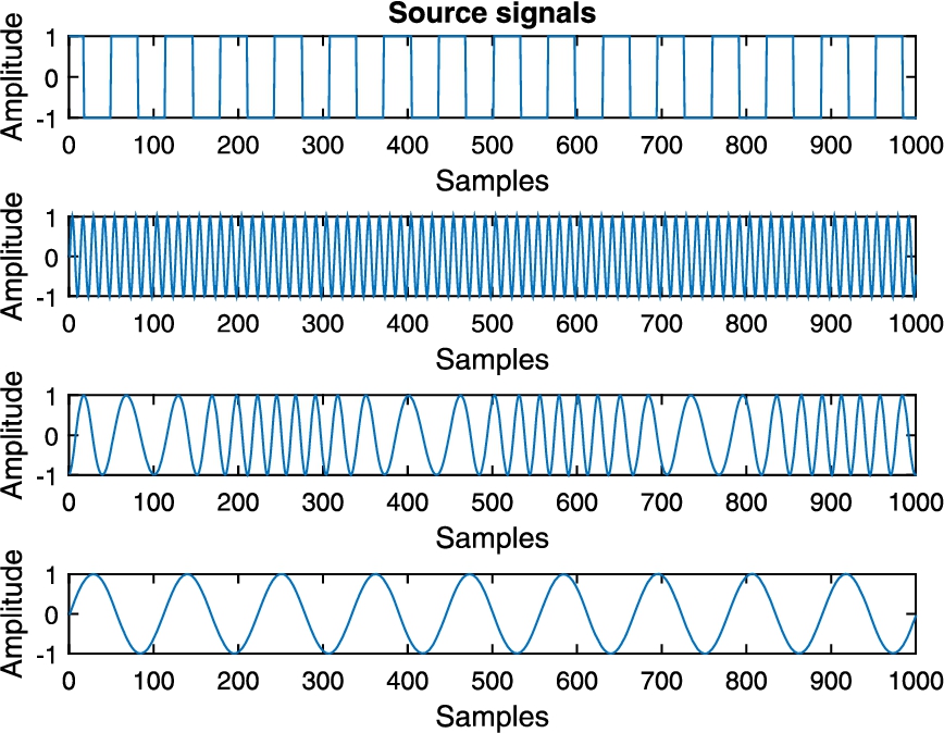
Fig. 3

The estimation of source signals.

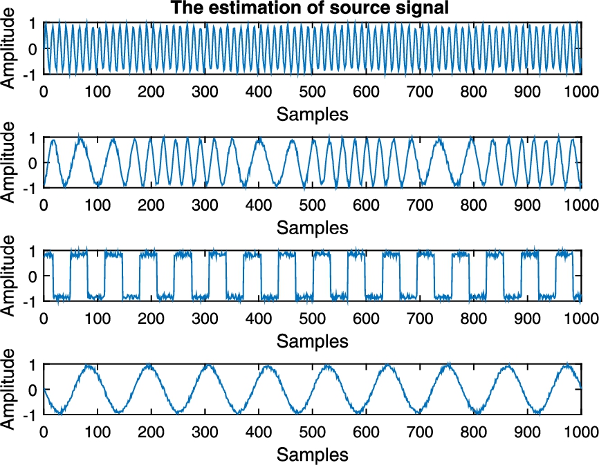
Figure 2 shows the source signal waveforms. Figure 3 shows the estimated signal waveforms of the source signals during the process. It can be clearly observed that the estimation of the source signals are quite similar to the source signals, which indicates the effectiveness of our proposed algorithm.

The former experiment was established under positive definite conditions. In this case, we evaluate the algorithm in over-determined conditions, and the source signal vector becomes:

St=[sin(1600πt),sin(180πt)]T.[TeX:] \[ {\mathbf{S}_{t}}={\big[\sin (1600\pi t),\hspace{2.5pt}\sin (180\pi t)\big]^{T}}.\]

The mixed matrix becomes A=randn(4,2)[TeX:] $\mathbf{A}=\texttt{randn(4,2)}$, and the number of samples is 16,000. The remaining experimental conditions remain unchanged. The 500 Monte Carlo trials are run, and convergence curves of the estimated value and the theoretical value of are shown in Fig. 4. As can be seen from Fig. 4, compared with the conventional algorithm, our proposed algorithm has a faster convergence rate and a smaller convergence value. Obviously, our proposed algorithm can still work well in the case of an over-determined model.

Fig. 4

Average performance index in an over-determined model.

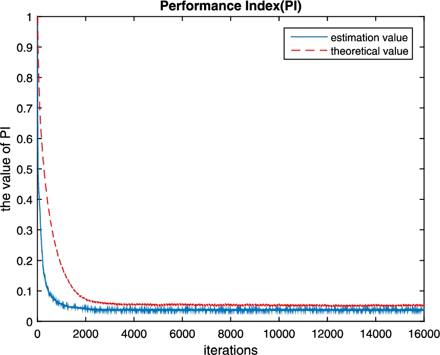
Fig. 5

Average performance index of the proposed algorithm and the conventional algorithm.

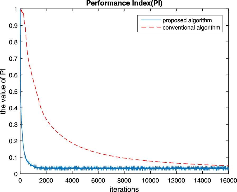
In order to indicate the advantage of our proposed algorithm in terms of convergence rate, we apply to the conventional algorithm proposed by Zhang et al. (2011) to the same data set. The 500 Monte Carlo trials are run, and the comparison curves of crosstalk error in iterative process is shown in Fig. 5. From Fig. 5, we can see that the conventional algorithm proposed by Zhang requires about 15,000 iterations to achieve convergence, but our proposed algorithm only requires about 1800 iterations. Obviously, our proposed algorithm increases the convergence rate more than eight times relative to the conventional algorithm proposed by Zhang.

4.2Real World Signals Experiments

In the real word signals experiments, a set of actual signals are used to test the proposed algorithm. The experimental environment is shown in Fig. 6. The signal transmission system consists of a signal generator and four transmitting antennas. The signal receiving system is made up of a signal receiver and four-element antenna array.

Fig. 6

The experiment setup.

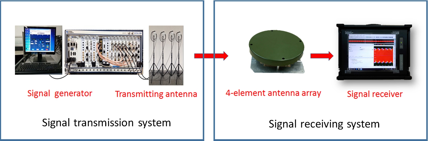
In the test, the signal generator generates single-frequency signals that are transmitted through the transmitting antennas, and then the signal receiver receives the mixed signals using the four-element antenna array. The sampling frequency is set to 62 MHz. We select 16,000 sampling points to compute the crosstalk error. The experimental result is shown in Fig. 7. It can be clearly observed that the convergence value of the proposed algorithm is smaller than that of the conventional algorithm and the convergence rate of the proposed algorithm is far better than the conventional algorithm. It demonstrates that the proposed algorithm is effective in practical experiment.

Fig. 7

Average performance index of the proposed algorithm and the conventional algorithm in a real world experiment.

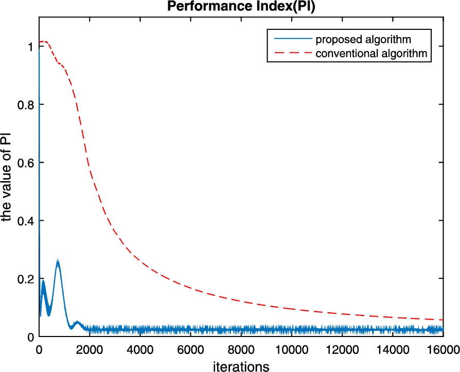
From the above experiments, we can know that the proposed algorithm for calculating the crosstalk error not only improves the robustness and the convergence rate of the crosstalk error greatly, but also deduces the crosstalk error to practical applications.

5Conclusion

At present, the crosstalk error is widely used to verify the validity and stability of the BSS algorithms in the simulation conditions. However, in the real application environment, it is impossible to know the global separation matrix of the signal in advance. Therefore, this criterion cannot be used in practice. In this paper, the crosstalk error calculation model is established based on the RLS algorithm, and the calculation method of the crosstalk error is deduced as an adaptive algorithm without prior knowledge by using real-time estimating of the global separation matrix. It can greatly extend the use scope of the crosstalk error. At the same time, a new crosstalk error definition is proposed to improve the robustness and convergence rate of the original crosstalk error. Finally, the experimental results show that the method proposed in this paper can predict the convergence trend of the crosstalk error well, which indicates the validity and robustness of the method proposed in this paper.

References

1 | Amari, S.I. ((1997) ). Neural learning in structured parameter spaces-natural Riemannian gradient. In: Advances in Neural Information Processing Systems, pp. 127–133. |
2 | Aroudi, A., Mirkovic, B., De Vos, M., Doclo, S. ((2016) ). Auditory attention decoding with EEG recordings using noisy acoustic reference signals. In: 2016 IEEE International Conference on Acoustics, Speech and Signal Processing (ICASSP). IEEE, pp. 694–698. |
3 | Basak, J., Amari, S.I. ((1999) ). Blind separation of uniformly distributed signals: a general approach. IEEE Transactions on Neural Networks, 10: (5), 1173–1185. |
4 | Bridwell, D.A., Rachakonda, S., Silva, R.F., Pearlson, G.D., Calhoun, V.D. ((2018) ). Spatiospectral decomposition of multi-subject EEG: evaluating blind source separation algorithms on real and realistic simulated data. Brain Topography, 31: (1), 47–61. |
5 | Choi, S., Cichocki, A. ((1997) ). August. Adaptive blind separation of speech signals: Cocktail party problem. In: International Conference on Speech Processing, pp. 617–622. |
6 | Cichocki, A., Amari, S.I. ((2002) ). Adaptive Blind Signal and Image Processing: Learning Algorithms and Applications, Vol. 1. John Wiley and Sons. |
7 | El-Sankary, K., Asai, T., Motomura, M., Kuroda, T. ((2015) ). Crosstalk Rejection in 3-D-Stacked Interchip Communication With Blind Source Separation. IEEE Transactions on Circuits and Systems II: Express Briefs, 62: (8), 726–730. |
8 | Grellier, O., Comon, P. ((1998) ). Blind separation of discrete sources. IEEE Signal Processing Letters, 5: (8), 212–214. |
9 | Jiang, X. ((2014) ). Blind signal separation for fault analysis of 400 Hz solid-state power supply. In: 2014 33rd Chinese Control Conference (CCC). IEEE, pp. 3213–3218. |
10 | Laheld, B., Cardoso, J.F. ((1993) ). Separation adaptative de sources en aveugle. Implantation complexe sans contraintes. In: Actes du XIVeme Colloque GRETSI, pp. 329–332. |
11 | Li, S., Sejnowski, T.J. ((1995) ). Adaptive separation of mixed broadband sound sources with delays by a beamforming Herault–Jutten network. IEEE Journal of Oceanic Engineering, 20: (1), 73–79. |
12 | Li, Z., Feng, Z.P., Chu, F.L. ((2012) ). A performance index of blind source separation based on improved crosstalk index. Zhendong yu Chongji (Journal of Vibration and Shock), 31: (18), 83–88. |
13 | Macchi, O. ((1993) ). Self-adaptive source separation by direct and recursive networks. In: Proceedings International Conference on Digital Signal Processing (DSP’93) Limasol, Cyprus, pp. 1154–1159. |
14 | Macchi, O., Moreau, E. ((1999) ). Adaptive unsupervised separation of discrete sources. Signal Processing, 73: (1–2), 49–66. |
15 | Mansour, A., Kawamoto, M., Ohnishi, N. ((2002) ). A survey of the performance indexes of ICA algorithms. In: Proc. IASTED Int. Conf. on Modelling, Identification and Control (MIC), pp. 660–666. |
16 | Mirzal, A. ((2017) ). NMF versus ICA for blind source separation. Advances in Data Analysis and Classification, 11: (1), 25–48. |
17 | Moreau, E., Macchi, O. ((1996) ). High-order contrasts for self adaptive source separation. International Journal of Adaptive Control and Signal Processing, 10: (1), 19–46. |
18 | Moreau, E., Macchi, O. ((1998) ). Self-adaptive source separation. II. Comparison of the direct, feedback, and mixed linear network. IEEE Transactions on Signal Processing, 46: (1), 39–50. |
19 | Nandakumar, M.M., Bijoy, K.E. ((2014) ). October. Performance evaluation of single channel speech separation using non-negative matrix factorization. In: 2014 National Conference on Communication, Signal Processing and Networking (NCCSN). IEEE, pp. 1–4. |
20 | Parra, L., Sajda, P. ((2003) ). Blind source separation via generalized eigenvalue decomposition. Journal of Machine Learning Research, 4: , 1261–1269. |
21 | Qian, X., Chunsheng, L., Jinfang, C. (2006). Adaptive algorithm for blind source separation from instantaneous noisy mixtures. Journal of Data Acquisition and Processing, 1–8. |
22 | Yang, H.H. ((1999) ). Serial updating rule for blind separation derived from the method of scoring. IEEE Transactions on Signal Processing, 47: (8), 2279–2285. |
23 | Yang, H.H., Amari, S.I. ((1997) ). Adaptive online learning algorithms for blind separation: maximum entropy and minimum mutual information. Neural Computation, 9: (7), 1457–1482. |
24 | Yatabe, K., Kitamura, D. ((2018) ). April. Determined blind source separation via proximal splitting algorithm. In: 2018 IEEE International Conference on Acoustics, Speech and Signal Processing (ICASSP). IEEE, pp. 776–780. |
25 | Zhang, T., Li, L., Zhang, G., Gao, C., Hou, R. ((2011) ). Use estimation of performance index to realize adaptive blind source separation. In: 2011 4th International Congress on Image and Signal Processing (CISP), Vol. 5: . IEEE, pp. 2322–2326. |
26 | Zhu, X.L., Zhang, X.D. ((2002) ). Adaptive RLS algorithm for blind source separation using a natural gradient. IEEE Signal Processing Letters, 9: (12), 432–435. |