
Simulation of diffusion using a modular cell dynamic simulation system
Abstract
A variety of mathematical models is used to describe and simulate the multitude of natural processes examined in life sciences. In this paper we present a scalable and adjustable foundation for the simulation of natural systems. Based on neighborhood relations in graphs and the complex interactions in cellular automata, the model uses recurrence relations to simulate changes on a mesoscopic scale. This implicit definition allows for the manipulation of every aspect of the model even during simulation. The definition of value rules ω facilitates the accumulation of change during time steps. Those changes may result from different physical, chemical or biological phenomena. Value rules can be combined into modules, which in turn can be used to create baseline models. Exemplarily, a value rule for the diffusion of chemical substances was designed and its applicability is demonstrated. Finally, the stability and accuracy of the solutions is analyzed.
1Introduction
The simulation of complex physical, chemical, and biological phenomena has become an important tool for the research in life sciences. Models that mimic the behavior of natural systems support the understanding and analysis of laboratory experiments [1]. In systems and cell biology such models are valuable for inferring the life-sustaining chemical transformations in cells [2], the self-organization of the cytoskeleton synthesis [3], and phenotypes of whole organisms [4]. Quantitative models are able to give actual predictions about the quantities in a system. Most models are generally systems of ordinary or partial differential equations (PDE). Such systems are composed of multiple equations, where each equation represents the concentration of a chemical compound. It is of high importance to model these equations as accurately as possible to correctly capture the phenomena observed on the biological level. Even small differences in the initial conditions may produce large discrepancies between the simulation and the experimental outcome [5]. Hence, each experimental model has to be addressed differently, and many parameters have to be measured and set to describe the phenomenon observed under specific conditions. While helpful for a small group of scientists, those models can rarely be adapted for problems that are the result of a similar underlying phenomenons [6]. Scientists can only observe consequences of physical and chemical laws that are entangled in complex systems such as cells and organisms. So it is no surprise, that most models do not describe the “real shape” of the problem and only characterize the guise of the phenomenon. For an illustration of the problem, consider a medical doctor who tries to cure an illness. Only by approaching and treating the underlying causes, he can hope to cure the patient. Treating the symptoms is only viable in the most severe cases. Similarly, if we are able to characterize the processes in a cell and know their interactions, it is possible to modify the system and obtain the behavior that is required. The creation of new fundamental laws is a large step in the development of systems biology [7]. Modeling those fundamental processes and combining them as system-theoretic concepts is still one of the greatest challenges in the field of systems biology [8, 9].
One technique to explore the general traits of interacting systems and spatio-temporal patterns are cellular automata (CA). Originated in the 1940s, CA are simulations discrete in time, space, and state. By applying a simple set of rules – which depend on automata elements, so-called cells, and their respective associations between each other – at each time-step, remarkably complex behaviors emerge from such automata [10, 11]. This discrete character to CA is tailored for the computation using traditional computers that operate at finite precision by design. Dynamic Cellular Automata, as an agent-based adaptation of CA, have been shown to describe a multitude of different cellular or biochemical processes [12]. Although CA have been used in many fields of biology [13], they played a minor role in recent years, because powerful tools such as ECell [14] and VCell [15] started to dominate the research field. Both tools and many others alike are based on PDEs that are composed and specified by the user of the software. With all reactions and processes defined, a numerical solution of the system of PDE is generated and calculated. The user is able to inspect the results and adjust parameters to fine-tune the model to fit the results gained via laboratoryexperiments.
Space is one of the key components when modeling the processes in cells. In the last decade simulations in systems biology have been moving from temporal-only models to spatio-temporal models [16]. An established practice for simulations with a spatial component is to partition the simulation space into smaller compartments that are able to exchange components or information. This holds true for CA, which are traditionally defined to handle spatial neighborhood relations on two- or three dimensional geometric tilings. The neighbors of each cell are defined by adjacent edges or corners.
Another approach to model natural systems are stochastic simulation algorithms (SSA) such as Chemical Master Equations (CME), which can be necessary when biological phenomena depend on stochastic fluctuations [17]. CME are able to model diffusion using particle position distributions – which are either compartment-based or reliant on Smoluchowski equations – and chemical reactions, based on probabilities of molecular reactions during a defined time period. Assuming a spatially homogeneous system the changes in concentration can be simulated.
PDEs, SSA and CA represent different techniques to explore the behavior of dynamic systems, all designed to define the change that occurs in events or time steps. In PDEs this change is explicitly defined from the starting point and for all following steps in time. Therefore it is possible to poll the state of the system by solving a single equation. In comparison, using CA, numerical methods, or SSE the next state of the system is implicitly defined by its current state, thus adjusting parameters or even states can be accomplished readily at every time step, but every state in between the current and the required time step has to be calculated [18, 19]. This leads to a consideration of the advantages and disadvantages of implicit definitions in opposition to explicit definitions. The updating procedure of explicit systems depends on the value of the previous time step, and may even be analytically formulated as a closed form solution. Therefore the determination of the updates is straightforward and computationally inexpensive. As a compromise, explicit methods are only conditionally stable, meaning errors at any stage of the computation or divergence in the starting conditions are amplified and not attenuated as the simulation progresses. Hence, explicit solutions require very small time steps, especially when there are major changes in a short time period. Implicit systems can include values of the current and previous time steps. The calculations performed in each time step are generally more difficult, resulting in a higher time complexity of the simulation. Nevertheless, implicit schemes are stable and can tolerate larger time steps than explicitly defined systems [20]. This also includes a robustness to unexpected changes. Especially in biological environments the ability to respond and adjust to spontaneous disturbances, such as molecular signals from other cells or changes in temperature is vital in order to create a realistic and robust model [21].
In 2001 Tomita proposed that systems biology should rise to a grand challenge of the 21st century [22]. The construction of a mathematical model of the whole cell is a key aspect in this challenge. In order to understand the complex system of the cell, the fundamental processes that govern its behavior have to be understood. A modular system that allows to easily add and remove certain aspects of a model is a possible approach to analyze the forces that drive biological systems. A seed model can be used as a basis to experiment with different pathways, reaction types, and parameter sets, without the need to modify the entire system due to adding a single component. To evaluate the possibilities that CA offer for modularized spatio-temporal modeling of natural systems, we define a graph-oriented CA and design a function to simulate diffusion processes. The diffusion of six different molecules within a rectangular shaped space is simulated with the model proposed in this paper and validated with a numerical approach. We discuss the stability of the solutions gained concerning different time and space resolutions and suggest a general guideline to select those parameters. In systems that simulate multiple chemical components and/or multiple phenomena, it can be difficult to select the best size for the time step. In numerical analyses different algorithms are available to estimate a stable step width, such as Ruge-Kutta methods [19]. With the proposed model it is possible to determine the time and spatial step size, without additional estimation methods. The user of the model has the freedom to weigh and choose between simulation accuracy, complexity, and stability before performing the simulation of the system.
2Methods
The concept of cellular graph automata has been pioneered by Angela Wu [23] in the late 1970s. The research with graph automata was mainly focused on investigating the properties of graphs and applications to graph grammars. Nevertheless, the dynamic definition of neighborhood in CA is a powerful aspect to capture geometries that cannot be defined easily by a static geometric definition.
2.1Modeling cellular graph automata
The definition of cellular d-graph automata proposed by Wu and Rosenfeld [23] has been adapted for this work. For reference purposes we will present a short informal definition. A d-graph Γ is a graph with labeled nodes and numbered edges. A distinguished label element # exists – if a node is not labeled with # it has exactly d edges emanating from it. Further a finite-state automaton M on d-graphs is defined as a double (Q, δ), where Q is a nonempty set of states and δ the transition function, which maps a new state to a node depending on the current state, the edge numbers and neighbor states. Further, the cellular d-graph automaton
For the adaption of cellular graph automata (CGA) presented here, we exchanged the definition of d-graphs with finite graphs, that are triplets (X, U, α) where X and U are two finite disjoint sets and α is a function [24]. This implies that nodes and edges are no longer labeled and do not rely on a bounded degree d. Additionally, the states Q is introduced at the level of CGA, because they are globally defined.
Definition 1 (Cellular Graph Automaton). Let a cellular graph automaton be a quadruple CGA = (V, E, Q, α), for which:
· V is a finite set of graph automaton cells,
· E is a finite set,
· Q is a finite set, and
· α : E ↦ V ∪ V is a partial function.
V, E, and Q are disjoint sets. The set V contains the nodes of the graph with elements denoted as v1, v2, …, vn and each element of this set is a graph automaton cell (see Definition 2). Elements e1, e2, …, eu originate from the set of edges E. The set Q = {q1, q2, …, qr} is the set of possible states. The number of elements in each set is given as n = |V|, u = |E|, and r = |Q|. The function α (ei) = (vj, vk) assigns the relation between a pair of nodes vj, vk ∈ V and an edge ei ∈ E. If such a relation exists between two nodes vj, vk they are called neighbors.
A graph automaton cell (GAC) is a modified version of the finite state automaton M, where we keep the essence of the transition function δ.
Definition 2 (Graph automaton cell). Let a graph automaton cell be a triple GAC = (p, δ, q), for which
·
· δ : Q* ↦ QCGA is a total function (the state rule), and
· q ∈ QCGA is the current state.
The position of a node in a space of dimension g is represented by the position
CGA are composed of nodes, and unlike CA, their neighborhood relations are based upon the connections represented by edges. Let dN be the neighborhood distance of two nodes. In other words: dN defines the number of edges on the shortest path between two nodes. Therefore the distance dN between two nodes vk, vj ∈ V, is dN (vk, vj) =1, if and only if there exists an edge e ∈ E such that α (e) = (vk, vj). Further, the distance dN between two distant nodes v1, vn ∈ V can be defined by the shortest path between them. Hence let (v1, v2, …, vn) ∈ V × V × ⋯ × V be the shortest path between two nodes, such that vi is neighbored to vi+1 for 1 ≤ i < n. The resulting distance will be dN (v1, vn) = n - 1. In contrast to CA, CGA do not define specific boundary conditions. Different pseudo boundaries can be created be adding new edges that specify the desired interactions.
While CA operate in a predefined tiling, GAC act depending on their neighbors, defined by α and represented by a multiset N. Let the multiset N, called neighbor states, be a double N = (Q, m), for which Q is the finite set of states and
The cardinality of the multiset is the sum of all multiplicity functions and equal to the degree deg of the node vk:
As an example consider a node vk in state q1 with three neighboring nodes in q3 and one neighbor also in state q1. The available states consist of QCGA = {q1, q2, q3}. The resulting multiset of neighbor states is Nvk = {q1, q1, q1, q3} and the appropriate functions are m (q1) =3, m (q2) =0 and m (q3) =1.
The transition of a node from one state q (t) at time t to the next state q (t + Δt) is defined by the state rule δ, which can be either deterministic or stochastic. The step size Δt is uniform. The domain Q* of δ is a multiset of states from QCGA that consists of the neighbor states Nvk, in addition to the state of node vk itself and maps to the next state q (t + Δt) of vk. An exemplary deterministic transition function would be:
This deterministic transition function determines the next state of a node, by the number of neighboring nodes in a certain state. If the number of nodes in state q1 is larger than the number of nodes in state q2 the next state of this node will be q1 and vice versa. The state q3 would be assigned if the number of nodes in q1 and q2 are exactly even.
With these definitions the state of a node can be set. Considering the initial representation of nodes as a segment of space inside of a biological system, possible states could be comprised of the environment or compartment a node is enclosing. In this context, the state of a node may be any organelle, such as chloroplast, endoplasmic reticulum, or Golgi apparatus. The states or objects can be allowed to move through the cell with rules adapted from the String definition in [26] or remain static. In order to handle continuous values, such as concentrations of species, the previous definition is augmented to Extended Graph Automaton Cells (EGAC), which are used to enrich the concept of CGA. Here, each node is able to accommodate a set of entities that represent its content.
The description species is used to generally refer to sets of atoms, molecules, molecular fragments, ions and similar entities, subject to a chemical process or to a measurement. Each species s ∈ S represents such a chemical compound. A value function
Definition 3 (Extended graph automaton cell). An extended graph automaton cell is a quintuple EGAC = (δ, Ω, q, W), for which
·
· δ : Q* ↦ QCGA is a total function (the state rule),
· Ω is a set of functions ω : W* × s ↦ W (the value rules),
· q ∈ QCGA is the current state, and
· W is the current value set.
The Definition 2 of GAC also applies to the multiset Q*, the transition function δ and the current state q. The value functions Ω and the current current value set W are new components to this definition. The value set W contains the sets of values defined by each value function
The domain W* of each value rule ω consists again of the neighboring value sets. Each value set Wvi of the nodes vi that share an edge with the node vk is included in the Mvk set.
The set of value rules Ω contains all value rules that are to be applied to the value set of the node vk. A single value rule ω maps from the set of multiple value sets W*, including neighbor value sets Mvk and the node vk itself, to the new value set W. A rule ω is used to calculate the change of any fi (t, v, s) of a species s, at node v and time t. For example, the arithmetic mean of the concentrations in a node can be assigned with:
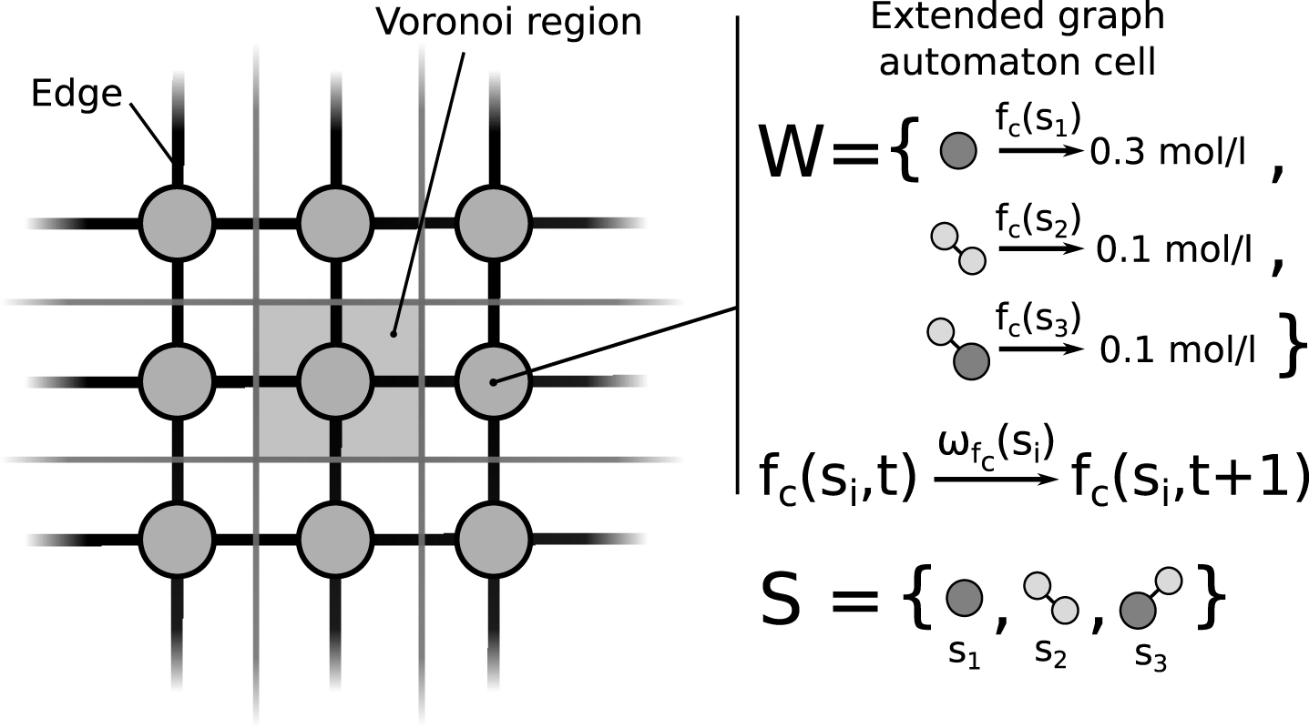
Fig.1
A section of a cellular graph automaton illustrating nodes, edges, and Voronoi regions. A set of species S is globally defined and a set of attributes can be assigned to every individual species. Each extended graph automaton cell (see Definition 3) contains the current concentration fc (si) of a species si. The species and values depicted were only chosen as an example. The value function ωfc (si) defines a rule for the change in concentration for each species.
The idea behind this definition is the creation of multiple value rules that represent natural phenomena inside of the cell. It is possible to define multiple value rules that modify the same value in a value set. For example, consider the diffusion of a species into neighboring compartments in addition to the conversion into another species during a chemical reaction. Both events would modify the concentration of the same species. In this case the sum of the changes for each species and value function will be applied to the node.
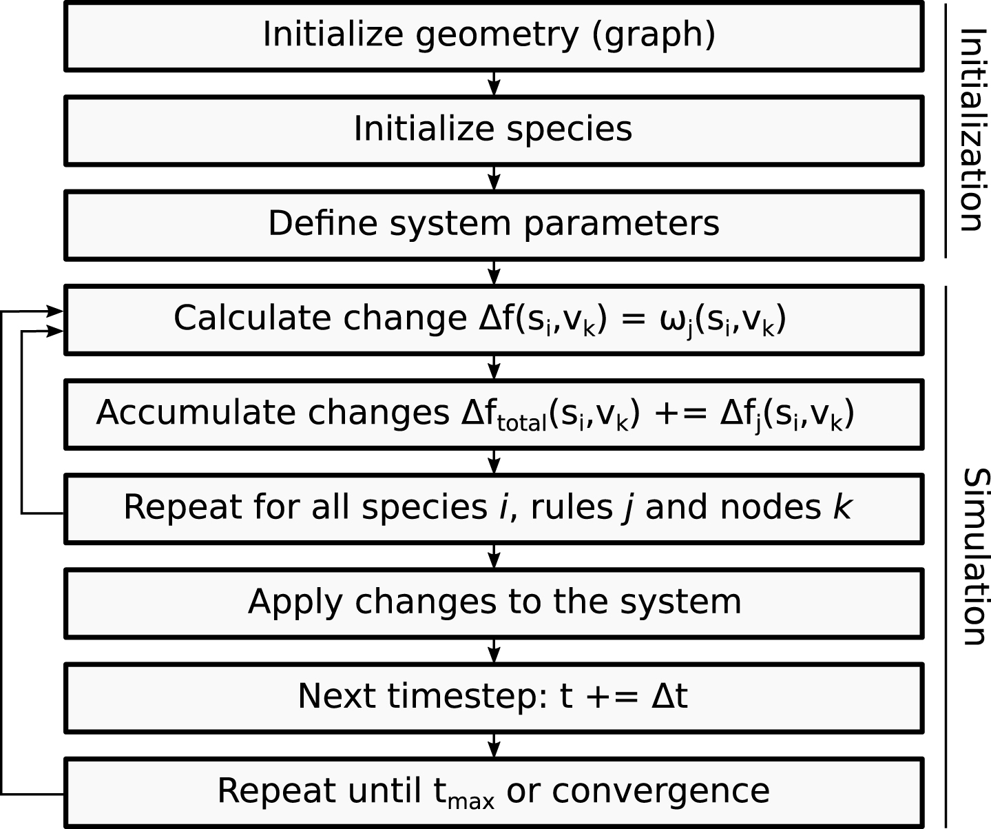
The size of the time step is uniform and can be parametrized as described in Section 2.3. This enables the simulation of multiple time scales depending on the phenomenon that is to be addressed. Additionally, the size of the time step provides the possibility to choose between a more accurate prediction (using numerous small time steps) or a faster simulation (using fewer large time steps). A schematic representation of the sequence of operations that are needed to setup and perform a simulation is depicted in Fig. 2.
Fig.2
The flowchart describes the general sequence of steps during the initialization process and actual simulation of CGA.
To evaluate the proposed model, the process of diffusion has been implemented as a value rule ωDif. Diffusion is one of the fundamental processes that governs the behavior of all natural systems on a molecular level. It is possible to derive an implicit value rule that is able to describe the flow of matter between the nodes in CGA. The derivation of this rule is presented in the following section.
2.2Modeling diffusion
Diffusion is a natural physical process in which molecules disperse from an area of high concentration proportional to a concentration gradient. This phenomenon is describes the random motion of all particles in solutions, called Brownian motion. Fick proposed the Second Law of Diffusion, in which the flux of matter in a liquid is proportional to the gradient of its concentration c scaled by a factor D [27]:
(1)
This equation needs to be transformed into a recurrence relation, which then enables the implementation into CGA. Using the finite differences method as shown in [20], the infinitesimal small steps in time ∂t and space ∂x can be formulated using finitely small steps Δt and Δx. The concentration was rewritten to c (t, x), to indicate its dependence on time t and the position x:
By calculating the limit with Δx, Δt → 0 of this function, it is possible to reformulate Fick’s second law in a discrete manner. The reformulation of the second space-derivative is performed specifically for CGA. Since the introduction of a neighborhood-oriented approach is required, it is necessary to distribute the spatial differences as uniformly as possible around the point of interest x, so that the isotropy of the geometric space is conserved. Subsequently, it is necessary to define the neighborhood of the current position x. Thus, let H = {h1, dotsb, hd} be the set of nodes that are adjacent to a node vk. This relationship is derived by collecting all nodes where dN (vk, hi) =1 (see Definition 1). In conclusion, position x will now be represented as a node vn and hi ∈ H are nodes, that have a distance of Δx = dN to vk. Since there is now a finite amount of neighbors, the concentration of each neighboring node needs to be considered:
Since the time scale of CGA is uniform and homogenous, it is possible to assume Δt = 1 and ΔdN = 1 without loss of generality if the nodes in the graph are arranged uniformly. When applying these terms, the previous equation results in:
Now it is possible to translate the equation to a value rule usable in CGA. The new concentration of a species s can be calculated with:
(2)
2.3Parameterizing and scaling
As mentioned in the definition of CGA, the spatial and time scales of CGA are dimensionless and uniform. The scaling factors that result from the true dimensionality of the system (time step size and node distance) have to be included in the value or transition rules, in order to affect the model system.
The diffusion coefficient D (s) represented by fd (s) is the only constant in the diffusion value rule ω (s) that connects the model system with specific characteristics of nature, and therefore provides an the opportunity to scale the diffusion value rule using node distance and the size of the time step. D is measured as a unit of area2 · time-1 and can be retrieved from literature or estimated from the molecular weight or volume. Hayduk and Laudie compiled a list of the diffusivities of 89 small molecules and developed a reliable correlation [28]. Young did the same for 143 proteins [29]. Using these correlations it is also possible to estimate the diffusion coefficient and in turn parametrize the simulation. In case of molecules the coefficient is often given in cm2 · s-1.
The distance between two nodes Δd and the length of a time step Δt has to be specified in order to simulate a defined environment (see Fig. 2). If these parameters are given, the diffusion constant D can be scaled to the size of the system. However, this requires the arrangement of nodes to be uniform across the covered space, so that dG (vj, vk) ∼ dN (vj, vk). We therefore propose the setup work flow depicted in Fig. 3. Ideally, the geometric distance dG is equal for all pairs of neighboring nodes and can therefore be used as Δd. The time step can be chosen depending on the environmental configuration. The final value of D, which is used and applied in CGA, is rescaled to represent Δt and Δd correctly. The scaled diffusivity
(3)
Fig.3
The first step to setup a simulation with cellular graph automata is to define the desired geometry of the system that one wants to simulate. Afterwards, the system is partitioned by covering it with a net-like graph. Each node is responsible for a subsection of space. Further adjustment methods can be applied to truncate and rearrange nodes, so that the true geometry is represented accurately. After the CGA has been adjusted to cover the simulation space, chemical species can be added to the system. Species and their attributes can be retrieved from databases such as ChEBI [35] or Pubchem [34]. For every node in the system the concentration can be set individually, a gradient qualitatively indicates nodes with a high concentration of a particular species in darker color and low concentrations in light color.
![The first step to setup a simulation with cellular graph automata is to define the desired geometry of the system that one wants to simulate. Afterwards, the system is partitioned by covering it with a net-like graph. Each node is responsible for a subsection of space. Further adjustment methods can be applied to truncate and rearrange nodes, so that the true geometry is represented accurately. After the CGA has been adjusted to cover the simulation space, chemical species can be added to the system. Species and their attributes can be retrieved from databases such as ChEBI [35] or Pubchem [34]. For every node in the system the concentration can be set individually, a gradient qualitatively indicates nodes with a high concentration of a particular species in darker color and low concentrations in light color.](https://ip.ios.semcs.net:443/media/isb/2017/12-3-4/isb-12-3-4-isb468/isb-12-isb468-g003.jpg)
2.4Verification
The viability of the simulated diffusion process, calculated by the implementation of the suggested model, is assessed in comparison to a numerical solution of the two-dimensional representation of the diffusion equation [30]. To compare the different approaches, the half-life τh was measured. In this context, τh is the time required for half of the concentration of the steady state to accumulate at a specified position. The half-life was used to contrast both approaches, since this measure is highly delicate and important to approximate the speed of the diffusion process [31]. Therefore, a good consensus between the predicted half-lives indicates a good overall compliance.
The sample system to be simulated was constructed as a square with a side length of 2500 nm. This square is partitioned into two rectangles with a width of 1250 nm (half of the system) and a height of 2500 nm. One of the rectangles is set up to have a starting concentration of 1.0 mol·l-1 and the other rectangle is set to a concentration of 0.0 mol·l-1. The system’s initial setup and progression is depicted in Fig. 4. Multiple species have been considered to assess the viability of the system. We have chosen some of the smallest molecules that may be of interest in cellular biology. Those species should be the most critical in the system because large quantities are moving between nodes. The diffusivity covers ranges from 4.40·10-5cm2·s-1 for hydrogen gas up to 6.40·10-6cm2·s-1 for ethane-1.2-diol (seeTable 1) [28].
Fig.4
A: The initial setup of the proposed experiment. A tube is filled with two solutions, separated by a central barrier. One half (indicated with light color) contains a high concentration of the proposed substance, the other half does not contain the solved substance. The distance between the barrier and the point of observation is the diffusion distance, for which the half life will be measured. To start the experiment the barrier is removed. Now the time is measured until half of the equilibrium concentration is reached at the point of observation. B: The initial setup of the rectangular graph automaton with twelve nodes side length. The nodes contain concentrations of 1.0 mol·l-1 (indicated with dark color) and 0.0 mol·l-1 (indicated with light color). C: A schematic depiction of the progression of the diffusion process of methanol at the point of observation. The half life is measured when the concentration reaches half of the equilibrium. This concentration of 0.25 mol·l-1 is indicated with a grey line. The coloring shown in the three boxes illustrate the state of the system at three points in time based on the experimental progression.
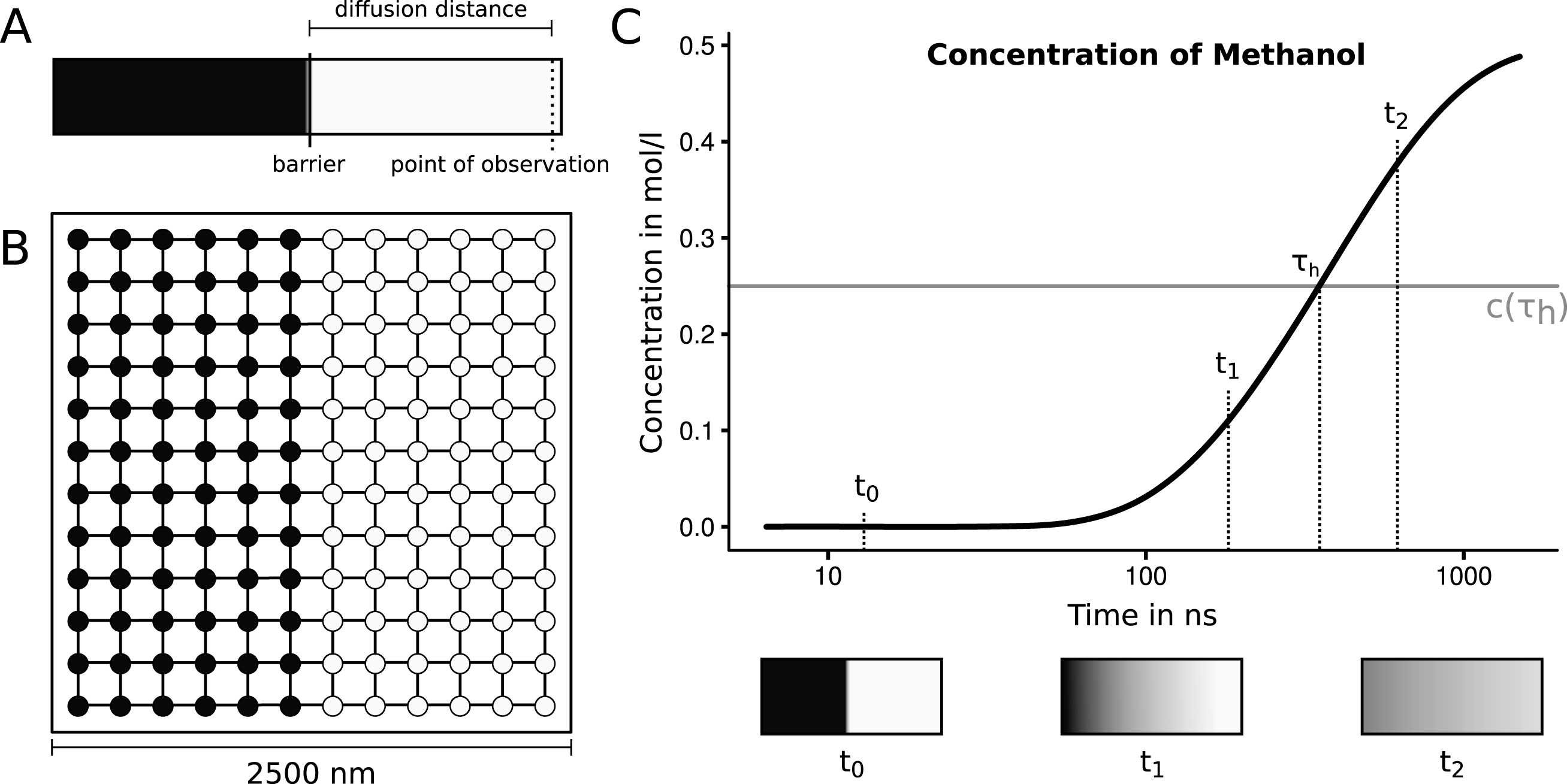
Table 1
Comparison of the simulation results
| Species | D (s) (
|
|
| Difference (ns / %) |
| Hydrogen gas | 4.40·10-5 | 135.9 | 131.8 | 4.1 / 3.07 |
| Ammonia | 2.28·10-5 | 262.2 | 254.3 | –7.9 / 3.09 |
| Methanol | 1.66·10-5 | 360.1 | 349.3 | –10.8 / 3.09 |
| Benzene | 1.09·10-5 | 548.4 | 532.0 | –16.4 / 3.08 |
| Succinic acid | 8.60·10-6 | 695.1 | 674.3 | –20.8 / 3.07 |
| Ethane-1.2-diol | 6.40·10-6 | 934.0 | 906.1 | –27.9 / 3.08 |
The graph automata simulation has been performed with 5 ns time steps and 40,000 nodes (200 x 200). The values for the diffusivity have been experimentally determined and are presented in [28].
Initially, a numerical approach was used to simulate the diffusion process in a closed system. This computation was performed using Octave [32]. The simulation uses an explicit finite difference method with a first order upwind in time and a second order central difference in space scheme [30, 33]. To specify the square shape of the simulation space, four reflecting Neumann boundaries were set. After specifying the systems boundaries, the kinematic viscosity of the system is set to exhibit the properties of the desired species ν = D (s). In the simulation, the concentrations of the far right side are observed and the system is simulated until it approaches the steady state c = 0.5 mol·l-1. Finally, the simulated half-life τh is measured.
Additionally, using the definition presented in this paper, a CGA is designed to simulate the same rectangular system (see Fig. 4B). The number of nodes at either side of the grid z is adjusted and the total number of nodes in the graph is |V| = z2. The global size of the system (2500 nm side length) will stay the same, only the distance between nodes Δd has to be recalculated for the scaling of the diffusion coefficient. Different automata were designed to assess the influence of node distance Δd and length of time steps Δt. Therefore 682 different systems have been simulated ranging from 10 to 70 nodes per side (using 31 samples in this range) and time steps of 10 ns to 1500 ns (using 22 samples in this range). Furthermore, these simulations have been performed for all mentioned species.
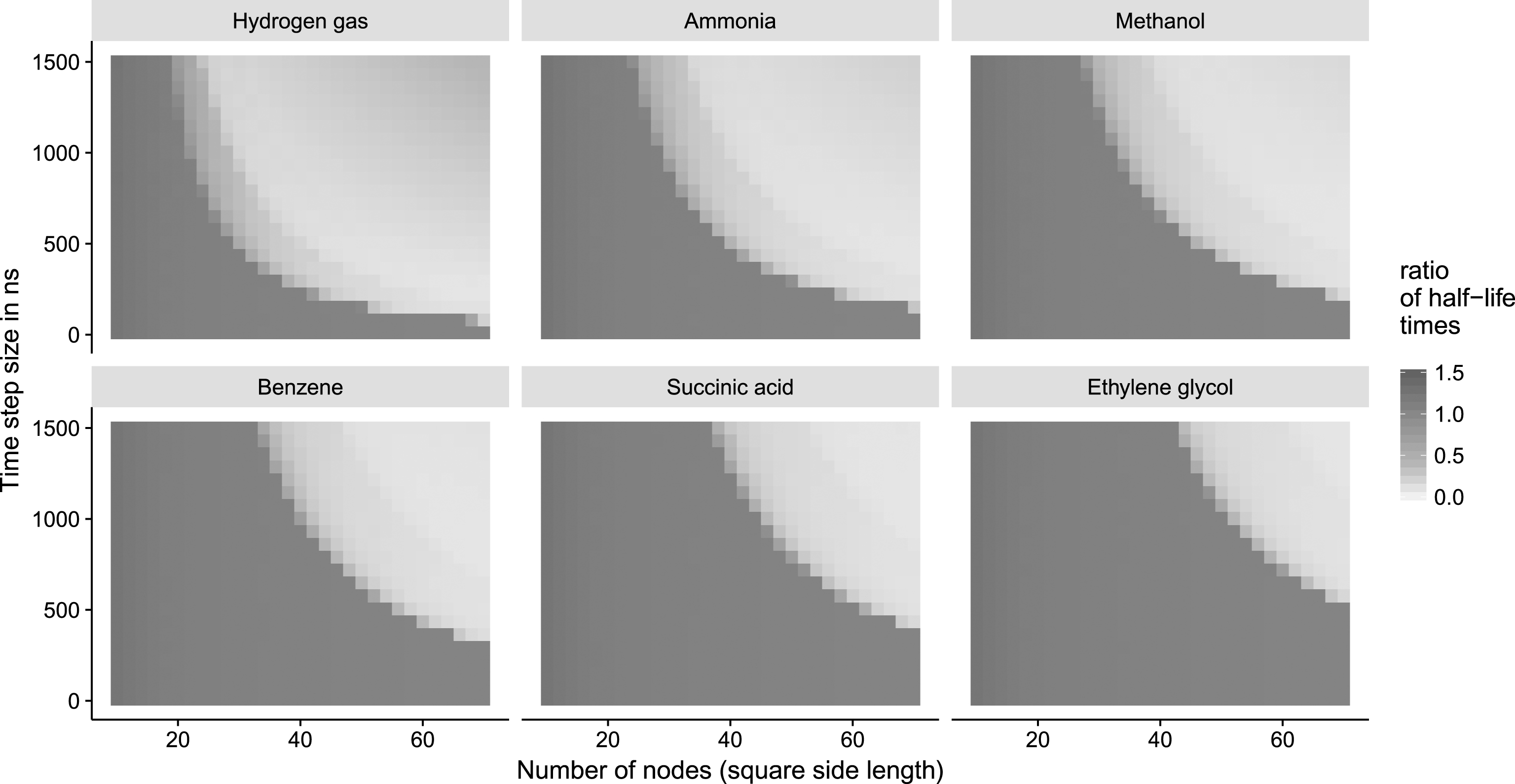
Fig.5
Simulations for six different substances. The number of nodes (side length of the square graph) ranges from 10 to 70 (implicitly changing the node distance Δd to maintain the overall simulation space) and the time step size Δt ranges from 10 ns to 1500 ns. Each dot corresponds to a simulation performed with different parameters for Δt and Δd. The ratio of the half life
3Results and discussion
A mathematical concept was developed that allows the simulation of multiple chemical species, subject to natural phenomena described by so-called value rules ω. The geometry of the model system is divided into multiple smaller subspaces that are simulated individually (see Fig. 3). Value rules are used to change the concentration of species inside of subspaces of the modeled system. The model itself is scale free, only the value rules have to be adjusted to the actual time and space regime of the simulation.
After the underlying geometry of the simulation is defined, chemical components can be added to each node of the system (see Fig. 3). Different attributes can be assigned to the chemical components that may be subject to change during the progression of the simulation. The diffusion requires the concentration and the diffusivity of each species. The concentration is node specific and will be changed during the simulation depending on the concentration of the surrounding cells, whereas the diffusivity is species specific and remains constant over time. The two global parameters that determine the scaling of the system are species and node independent. Those are the node distance ΔD (spatial step size) and the time step size Δt. Following the initialization of all required parameters, the simulation can be started. In each time-step the transition rules are applied and new values are set for the next iteration. A step-by-step progress of the setup of such a system is reenacted in Appendix A and another example for the implementation of value rules in the case of first order reactions is given in Appendix B.
The simulation system and model were implemented in order to verify their applicability. We developed the application programming interface Simulation of Natural Systems using Graph Automata (SiNGA) in the Java programming language. The source code is provided on GitHub under GNU General Public License Version 3 (see github.com/cleberecht/singa).
The results of an exemplary system (see Fig. 5) indicate, that the simulation using CGA with an increasing number of nodes and a decreasing time step size converge to the half life calculated with the numerical simulation. However, the graphs also show that the system is unstable when a large number of nodes (equivalent to small node distances Δd) is used in conjunction with large time steps. This is to be expected if the combined amount of concentration to be distributed among the neighbors in one time step is larger than the concentration a node currently contains. Hence, the time scale is underestimated and negative values ensue. Consequently, the initial setup of the system has to be done carefully. The dimensions of the system have to match the speed of the species with the highest diffusivity D (s). We derived the following threshold
(4)
that traces the arches that can be seen in Fig. 5. Here, let
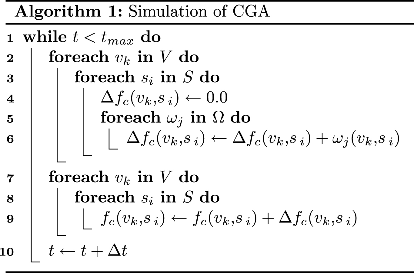
As depicted in the flowchart in Fig. 5 for every time step every node needs to be addressed at least once. The complexity of each time step is
4Conclusion
PDEs are an established strategy to simulate a variety of natural systems. In systems that have predictable behaviors and outcomes PDEs flourish to their full potential. In biology however, one often encounters systems that are very complex and influenced by multiple aspects. In these cases PDEs reach the limits of their applicability. Using implicit systems such as CA or CGA, it may be possible to simulate different systems that cannot be tackled efficiently using PDE.
With the proposed definition of CGA we have shown that it is possible to simulate diffusion of different chemical species to a high degree of accuracy. Diffusion is one of the most fundamental processes that many biological systems rely on. The system shown here is able to easily adjust to different time and space scales with little adjustments to the configuration of the system. Using the underlying structure of graphs it is possible to define different topologies. It is possible to add plenty of species to a simulation. Furthermore, the user is able to simulate and observe the system in order to improve the understanding of its current behavior. It is even possible to alter the concentration of a species at a specific node, or the structure of the graph at any point during the simulation, due to the implicit definition. Finally, not much mathematical understanding that is needed to set the system up (see setup process in Appendix A). As shown in Fig. 2, the user has to initialize the graph first, than choose the required species and finally define the systems parameters Δd and Δt. To guide the definition process of the parameters, the threshold (Equation 4) can be consulted. A trade-off can be chosen between accuracy and time complexity of the simulation. Hence, the end user can decide whether qualitative predictions are sufficient or precise simulations are required. Databases such as PubChem, ChEBI, or UniProt allow the automatic extraction of features for different species that are relevant for the estimation of critical parameters (such as the diffusivity) [34–36].
Computer simulations are able to act as a bridge between theory and experiment [37]. In the past the gap between theory and experiment for molecular behavior has been overcome by molecular dynamic simulations [38, 39]. However there is still a lot to be done to bring theory and experiment together when it comes to the dynamics of cellular processes. First steps were done by many researchers over the past centuries. Nevertheless, the gap between generalizable simulations and experimental outcome still needs to be closed. We hope that the different fields of science will work together to make a similar approach to “Cell Dynamic Simulations"possible.
In the near future, research will be directed towards the creation of value rules for different chemical reaction types and membrane transport. The setup process for simulations will be further simplified by providing possibilities to extract information from relevant databases and by offering visual feedback using the graphical user interface. Additionally the SiNGA application programming interface (available on GitHub github.com/cleberecht/singa) is under constant development.
Author contributions
All authors designed the research. C.L. designed and implemented the model and simulation strategy, and evaluated the performance. C.L. and F.H. wrote the paper.
Appendices
Appendix A. Simulation setup
Step 1: Definition of the target system. The layout of the underlying graph of the CGA is the first step in the setup of a simulation. The geometry and dimensionality of the target system has to be respected and eventually assumptions have to be made. A one dimensional system can be simulated by using a line of nodes, where each node is only connected to the next node. By also connecting the first and the last node of the system a periodic boundary condition in terms of regular cellular automata can be introduced. A two dimensional system can be composed in different ways, for instance by arranging four nodes around a central node (see example system in Fig. 4), a classical cellular automaton with a squared tiling can be recreated. It would also be possible to create a hexagonal tiling by introducing six neighbors to each node. Again, by connecting opposite sides of the system periodic boundary conditions are introduced. In theory the modeling of arbitrary dimensionalities should be possible depending only on the connection of nodes in the graph.
Example: For the purpose of this guide, a two dimensional system is chosen without periodic boundary conditions.
Step 2: Placement of the corresponding nodes. If the CGA should represent the actual geometry of a cell, a microscopic image can be used as a guideline to place the nodes of the graph. The number of nodes that are supplied in this step determine the accuracy of the system to a large extend. Each node is responsible for the simulation of a small region of space during the simulation. More nodes increase accuracy as well as runtime. Since the nodes need to be placed uniformly in the desired space a relaxation algorithms such as Lloyds Algorithm [40] should be applied and afterwards the nodes should be connected using a stringent distance cutoff. After this step the graph should uniformly span across the simulation space. Now the average distance between neighboring nodes is used to parametrize Δd.
Example: A simple square simulation space with an area of 100 mm2 is filled with 100 nodes. The large square is partitioned in 100 small squares, and at the center of each square a node is placed. Now the space is uniformly covered. Afterwards, neighboring nodes are connected and the distance between two nodes should be uniformly the same with Δd = 0.9 mm. The distance might seem surprising but is a result of the nodes being placed inside of the square and not on the border.
Step 3: Species selection and concentration assignment. Now the species of interest need to be specified and the concentrations have to be set. Each node requires a starting concentration.
Example: We might choose the molecule Benzene that has a concentration of 0.5 mol·l-1 in the two leftmost columns. Hence we set the value function fc (Benzene) = 0.5 for the corresponding nodes and fc (Benzene) = 0.1 for all remaining nodes.
Step 4: Choosing Δt and determining
Example: For the system that was introduced up to this point, the following threshold can be derived:
A node is neighbored to a maximum of four neighbors, the node distance has been set to 0.9 mm, and the maximal difference in concentration is 0.4 mol·l-1. Now the following three time steps will be considered: 1 s, 50 s and 100 s. To scale the experimentally determined diffusivity D (Benzene) = 1.09·10-5cm2·s-1 [28] to
Simulation. After the graph is constructed and the the time step size Δt, node distance Δd, and scaled diffusivity of all desired species are set, the simulation can begin. During simulation, the change for each node is calculated first using the the value rules ω. After all changes have been calculated, they are added to the previous values and the time step is increased.
Appendix B. Implementing value rules
The implementation of additional value rules is dependent on their requirement for neighboring values. If the value rule does not require information from neighboring values, its implementation is straight forward. As an example a simple case of chemical kinetics shall be demonstrated:
The general case of a first order reaction with two chemical species A and P and their stoichiometric coefficients a and p can be denoted in the form:
The reaction rate of a first-order reaction A → P can be described by:
• v is the reaction rate (in mol·l-1·s-1),
• c (S) is the concentration of a species s,
• k is the rate coefficient, and
• t is the time.
The differentials will be be transformed to discrete changes, to transition to CGA.
Further, the concentration will be rewritten to c (s, t), to describe c as a function depending on species and time:
Because of the uniformity of the time steps Δt can be set to 1:
Therefore the recurrence relation for the new concentration of a species S at t + 1 in a first-order reaction can be calculated with:
In this equation u (s) denotes the stoichiometric coefficient in the reaction that is to be simulated. The equation can be translated to a value rule in CGA notation, for which only the change is relevant:
Note that the rate of change is always calculated in dependence of the substrate concentration of the reaction sA, since if there is no actual substrate no reaction can occur. The rate coefficient k from literature or databases needs to be scaled to take the actual time step into account, that is to be applied in the concrete CGA with
Acknowledgments
This work was supported by the European Social Fund (ESF) and the Free State of Saxony, Germany. We would like to thank our colleagues, especially Sebastian Bittrich and Florian Kaiser, for thought-provoking impulses and fruitful discussions. Additional we thank Hannah Siewerts for proofreading and feedback on the manuscript.
References
[1] | Ventura B.D. , Lemerle C. , Michalodimitrakis K. and Serrano L. . Fromto in silico biology and back, Nature 443: (7111) ((2006) ), 527–533. |
[2] | Chassagnole C. , Noisommit-Rizzi N. , Schmid J.W. , Mauch K. and Reuss M. . Dynamic modeling of the central carbon metabolism of escherichia coli, Biotechnology and Bioengineering 79: (1) ((2002) ), 53–73. |
[3] | Nédélec F. , Surrey T. and Karsenti E. . Self-organisation and forces in the micro-tubule cytoskeleton, Current Opinion in Cell Biology 15: (1) ((2003) ), 118–124. |
[4] | Karr J.R. , Sanghvi J.C. , Macklin D.N. , Gutschow M.V. , Jacobs J.M. , Bolival B. , Assad-Garcia N. , Glass J.I. and Covert M.W. . A whole-cell computational model predicts phenotype from genotype, Cell 150: (2) ((2012) ), 389–401. |
[5] | Poincaré H. . Science and method. Courier Corporation, (2013) . |
[6] | Shuler M.L. , Leung S. and Dick C.C. . A mathematical model for the growth of a single bacterial cell, Annals of the New York Academy of Sciences 326: (1) ((1979) ), 35–52. |
[7] | Wolkenhauer O. and Mesarović M. . Feed-back dynamics and cell function: Why systems biology is called systems biology, Molecular BioSystems 1: (1) ((2005) ), 14–16. |
[8] | Mesarović M.D. . Systems theory and biology view of a theoretician, In Systems Theory and Biology, pages 59–87. Springer, (1968) . |
[9] | Villaverde A.F. and Banga J.R. . Reverse engineering and identification in systems biology: Strategies, perspectives and challenges, Journal of The Royal Society Interface 11: (91) ((2014) ), 20130505. |
[10] | Adami C. . Introduction to artificial life, volume 1: . Springer Science & Business Media, (1998) . |
[11] | Wolfram S. . A new kind of science, volume 5: . Wolfram Media Champaign, (2002) . |
[12] | Wishart D.S. , Yang R. , Arndt D. , Tang P. and Cruz J. . Dynamic cellular automata: An alternative approach to cellular simulation, In Silico Biology 5: (2) ((2005) ), 139–161. |
[13] | Ermentrout G.B. and Edelstein-Keshet L. . Cellular automata approaches to biological modeling, Journal of Theoretical Biology 160: (1) ((1993) ), 97–133. |
[14] | Tomita M. , Hashimoto K. , Taka-hashi K. , Shimizu T.S. , Matsuzaki Y. , Miyoshi F. , Saito K. , Tanida S. , Yugi K. , Venter J.C. . et al. E-cell: Software environment for whole-cell simulation, Bioinformatics 15: (1) ((1999) ), 72–84. |
[15] | Slepchenko B.M. , Schaff J.C. , Macara I. and Loew L.M. . Quantitative cell biology with the virtual cell, Trends in Cell Biology 13: (11) ((2003) ), 570–576. |
[16] | Lemerle C. , Ventura B.D. and Serrano L. . Space as the final frontier in stochastic simulations of biological systems, FEBS Letters 579: (8) ((2005) ), 1789–1794. |
[17] | Gillespie D.T. . Exact stochastic simulation of coupled chemical reactions, J Phys Chem 81: (25) ((1977) ), 2340–2361. |
[18] | Brin M. and Stuck G. . Introduction to dynamical systems. Cambridge University Press, (2002) . |
[19] | Mattheij R.M.M. , Rienstra S.W. and Thije Boonkkamp J.H.M.T. . Partial differential equations: Modeling, Analysis, Computation. Siam, (2005) . |
[20] | Johnson C. . Numerical solution of partial differential equations by the finite element method. Courier Corporation, (2012) . |
[21] | Csete M.E. and Doyle J.C. . Reverse engineering of biological complexity, Science 295: (5560) ((2002) ), 1664–1669. |
[22] | Tomita M. . Whole-cell simulation: A grand challenge of the 21st century, Trends in Biotechnology 19: (6) ((2001) ), 205–210. |
[23] | Wu A. and Rosenfeld A. . Cellular graph automata. i. basic concepts, graph property measurement, closure properties, Information and Control 42: (3) ((1979) ), 305–329. |
[24] | Rosenstiehl P. , Fiksel J.R. and Holliger A. . Graph theory and computing, chapter Intelligent Graphs: Networks of Finite Automata Capable of Solving Graph Problems, pages 219–265. Academic Press, (1972) . |
[25] | Aurenhammer F. . Voronoi diagrams – a survey of a fundamental geometric data structure, ACM Computing Surveys (CSUR) 23: (3) ((1991) ), 345–405. |
[26] | Chopard B. . A cellular automata model of large-scale moving objects, Journal of Physics A: Mathematical and General 23: (10) ((1990) ), 1671. |
[27] | Fick A. . Ueber diffusion, Annalen der Physik 170: (1) ((1855) ), 59–86. |
[28] | Hayduk W. and Laudie H. . Prediction of diffusion coefficients for nonelectrolytes in dilute aqueous solutions, AIChE Journal 20: (3) ((1974) ), 611–615. |
[29] | Young M.E. , Carroad P.A. and Bell R.L. . Estimation of diffusion coefficients of proteins, Biotechnology and Bioengineering 22: (5) ((1980) ), 947–955. |
[30] | Crank J. and Nicolson P. . A practical method for numerical evaluation of solutions of partial differential equations of the heat-conduction type, Advances in Computational Mathematics 6: (1) ((1996) ), 207–226. |
[31] | Axelrod D. , Koppel D.E. , Schlessinger J. , El-son E. and Webb W.W. . Mobility measurement by analysis of fluorescence photobleaching recovery kinetics, Biophysical Journal 16: (9) ((1976) ), 1055. |
[32] | Eaton J.W. , Bateman D. , Hauberg S. , Wehbring R. , GNU Octave version 4.0.0 manual: A high-level interactive language for numerical computations (2015) . |
[33] | LeVeque R.J. . Finite volume methods for hyperbolic problems, volume 31: , Cambridge university press, (2002) . |
[34] | Kim S. , Thiessen P.A. , Bolton E.E. , Chen J. , Fu G. , Gindulyte A. , Han L. , He J. , He S. , Shoemaker B.A. . et al. Pubchem substance and compound databases, Nucleic Acids Research, page gkv951, (2015) . |
[35] | Hastings J. , Matos P.D. , Dekker A. , Ennis M. , Harsha B. , Kale N. , Muthukrishnan V. , Owen G. , Turner S. and Williams M. . et al. The chebi reference database and ontology for biologically relevant chemistry: Enhancements for 2013, Nucleic Acids Research 41: (D1) ((2013) ), D456–D463. |
[36] | UniProt Consortium et al. Uniprot: A hub for protein information, Nucleic Acids Research, page gku989, (2014) . |
[37] | Allen M.P. . Introduction to molecular dynamics simulation, Computational Soft Matter: From Synthetic Polymers to Proteins 23: ((2004) ), 1–28. |
[38] | Karplus M. . Development of multiscale models for complex chemical systems: from h+ h2 to biomolecules (nobel lecture), Angewandte Chemie International Edition 53: (38) ((2014) ), 9992–10005. |
[39] | Levitt M. . Birth and future of multiscale modeling for macromolecular systems (nobel lecture), Angewandte Chemie International Edition 53: (38) ((2014) ), 10006–10018. |
[40] | Lloyd S. . Least squares quantization in pcm, IEEE Transactions on Information Theory 28: (2) ((1982) ), 129–137. |

