
Where Do CABs Exist? Verification of a specific region containing concave Actin Bundles (CABs) in a 3-Dimensional confocal image
Abstract
CABs (Concave Actin Bundles) are oriented against the scaffold transversally in a manner different from traditional longitudinal F-actin bundles. CABs are present in a specific area, and do not exist in random areas. Biologically, CABs are developed to attach cells to fibers firmly so that CABs are found near cells. Based on this knowledge, we closely examined 3D confocal microcopy images containing fiber scaffolds, actin, and cells. Then, we assumed that the areas containing high values of compactness of fiber, compactness of actin, and density of cells would have many numbers of CABs.
In this research, we wanted to prove this assumption. We first incorporated a two-point correlation function to define a measure of compactness. Then, we used the Bayes’ theorem to prove the above assumption. As the assumption, our results verified that CABs exist in an area of high compactness of a fiber network, high compactness of actin distribution, and high density of cells. Thus, we concluded that CABs are developed to attach cells to a fibrillar scaffold firmly. This finding may be further verified mathematically in future studies.
1Introduction
Jones et al. [1] investigated the in vitro interaction of both mature endothelial cells (ECs) and of less differentiated EC colony-forming cells to poly-ɛ-capro-lactone (PCL) fibers with diameters in 5-20μm range (scaffold micro-fibers (SMFs)). This range of diameters of fibers is within cell-size range.
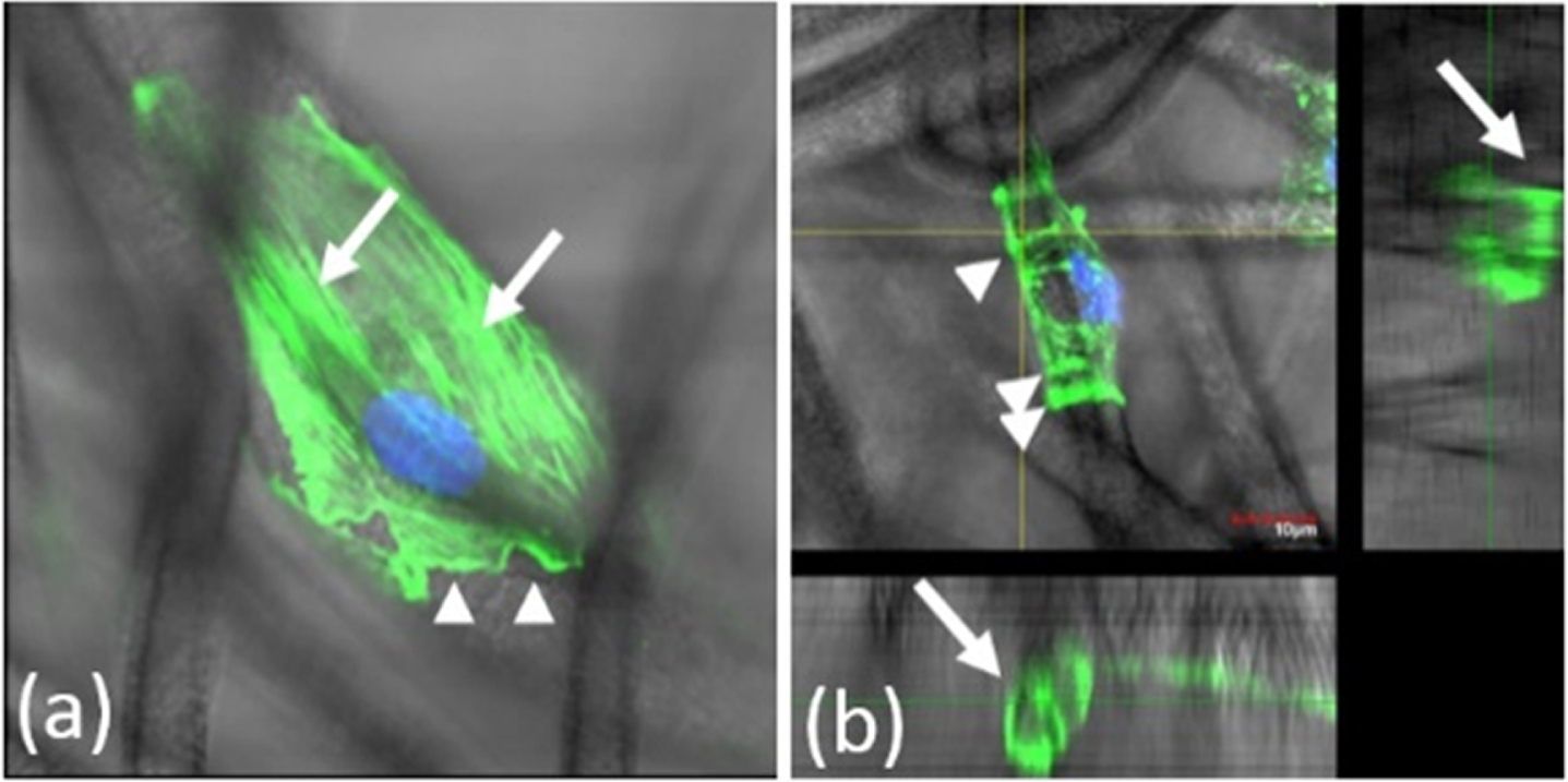
In their experiment, the researchers found that ECs wrap the SMFs completely, forming a cylindrical morphology. They further investigated the distribution of F-actin microfilaments in scaffold-wrapping ECs, to determine their circumferential extension. Figure 1 (a)-(b) shows cells incubated for a longer time with SMFs. They reported the full circumferential continuity of F-actin structures by unwrapping the image in Fig. 1 (c), which is shown as a ring-like pattern occasionally crossing the nuclei.
Fig. 1
Visualization of circular gripping of SMFs by F-actin in the human umbilical vein ECs (HUVECs) (Reproduced from [1]). (a)-(c) visualized F-actin in the HUVECS. (a) An original confocal image in 2D projection. A SMF portion containing F-actin bands of interest is marked by a yellow rectangle; (b) An enlarged image of the yellow rectangle in (a); (c) Left shows a vertically oriented image projection of (b). For comparison, we unwrapped the cylinder distribution of F-action to visualize full-circle continuity of F-actin around the SMF (right). Fig (d)-(f) are examples of F-actin rings in the interaction between a cell and a scaffold(s). (d) Full-wrapping of a fiber at the cell’s extremities (yellow line) by F-action bundles. The white scale is around 10μm; (e) F-actin in a SMF-attached cell. It contains AGs (arrowhead), an actin ruffle-like structure (arrow), and a blob with abundant actin (dashed arrow); (f) A cell is laid over three intertwining SMFs. The concentration of AGs is greater at all extremities than at the interior of the cell(arrowhead).
![Visualization of circular gripping of SMFs by F-actin in the human umbilical vein ECs (HUVECs) (Reproduced from [1]). (a)-(c) visualized F-actin in the HUVECS. (a) An original confocal image in 2D projection. A SMF portion containing F-actin bands of interest is marked by a yellow rectangle; (b) An enlarged image of the yellow rectangle in (a); (c) Left shows a vertically oriented image projection of (b). For comparison, we unwrapped the cylinder distribution of F-action to visualize full-circle continuity of F-actin around the SMF (right). Fig (d)-(f) are examples of F-actin rings in the interaction between a cell and a scaffold(s). (d) Full-wrapping of a fiber at the cell’s extremities (yellow line) by F-action bundles. The white scale is around 10μm; (e) F-actin in a SMF-attached cell. It contains AGs (arrowhead), an actin ruffle-like structure (arrow), and a blob with abundant actin (dashed arrow); (f) A cell is laid over three intertwining SMFs. The concentration of AGs is greater at all extremities than at the interior of the cell(arrowhead).](https://ip.ios.semcs.net:443/media/isb/2023/15-1-2/isb-15-1-2-isb210240/isb-15-isb210240-g001.jpg)
The median portion of cells often displayed only partial F-actin arcs, which are named “concave actin bundles” (CABs). In serial optical sections, CABs were found to co-exist with fully-wrapped F-actin bands, that were preferentially located towards cell margins (Fig. 1 (c)-(d)). CABs were either shorter than a half-circle and oriented obliquely to the axis of SMFs (Fig. 1 (d)), or longer than a semicircle and showing a more transversal positioning (Fig. 1 (e)), a grading that suggests their progression towards full circles. Where CABs represent full circles, they are named “actin grips” (AGs). Thus, AGs are special cases of CABs.
This wrapping is performed by adopting a cylindrical morphology, accompanied by the progressive reorganization of F-actin filaments in a ring-like pattern. This is a newly found type of organization of F-actin filaments mediating cell-matrix interactions. Thus, in the cells that intimately engaged individual SMFs, F-actin was distributed not only as classical stress fibers longitudinally aligned with the scaffold, but also as transversal rings, in a proportion that increased with the time in culture. Figure 2 shows these two types of organization of F-actin filaments. CABs (or AGs) are conspicuous F-actin bundles oriented transversally to scaffold’s fibers as shown in Fig. 2 (b) which is different from Fig. 2 (a).
Fig. 2
F-actin organization in cell-scaffold interaction. (a) An image of longitudinally aligned stress fibers (arrows). The arrowheads indicate F-actin containing ruffles. (b). A cross-sectional image of a supporting fiber. Concave actin bundles (CABs) (arrow) grip the fiber in a circular fashion. Green indicates F-actin. Blue indicates the nuclei.
Unlike stress fibers, CABs (or AGs) showed no co-localization with focal adhesions, or intermediate filaments. The grip formation depends on scaffold fiber diameter, with an optimum diameter around 10μm. Confocal and live-cell images showed that more grips were formed in cells which remained in culture longer, and that these cells were also less motile.
CABs helps understand how ECs solve their topological problem, when (literally) facing an unusual environment, and could also illuminate their behaviour in corresponding situations in vivo.
CABs are more dynamic structures than stress fibers. CABs also do not co-localize with the actin filaments oriented alongside the scaffold. Based on these observations, it was determined that CABs may contribute to the maintenance of an elongated endothelial morphology on the fibrillar support even in the absence of a FA-mediated adhesion, and that their dissolution may lead to cell shape modifications. These facts imply that CABs may supply (or replace) cells’ need for direct adherence, required for survival [2]. Further, CABs suggest a constrictive capacity, a function reserved only for cytokinesis furrows in ECs, and to the peri-vascular contractile cells (e.g. pericytes) [1].
Thus, CABs have multiple possible applications in tissue engineering, such as the stabilization of EC interaction with the scaffolds used as cell carriers, immuno-isolation of fibrillar scaffolds to mitigate their foreign body reaction, control of post-implantation immune responses, or controlling the differentiation of ECs via substrate-driven gene expression [1].
CABs are believed to exist for cell’s direct adherence to fibers, which provides to the attached cell essential mechanical properties. Thus, it seems that CABs exist around cells. However, we want to verity this fact, so that we may scrutinize an existential question: Where do CABs exist?
By closely probing 322 regions (which might contain a CAB) extracted by our previous algorithms described in [3] from 11 confocal image volumes (containing fiber scaffold, actin, and cells), we made a hypothesis of CABs’ existence: CABs exist largely in the area of high compactness of fibers, high compactness of actin, and high density of cells. In a confocal image volume, fibers were stained in red, actin in green, and cell in blue. We defined a fiber as a set of templates in our previous algorithms [3].
We calculated the density of fibers in the number of templates in a candidate CAB region. We calculated the density of actin as the number of green pixels in a CAB candidate region. Regarding cells, we segmented cells using the algorithm described in [4] and counted the number of pixels in the segmented cells. In the above hypothesis of CAB’s existence, if the number of templates, the number of green pixels, and the number of pixels in detected cells were above the experimental thresholds in a CAB candidate region in a confocal image volume, we defined the cases as ‘high’
If an area that has many numbers of fibers and those fibers cross each other intricately, the area has a high value of compactness of fibers. Similarly, if an area is widely and closely distributed with actin, the area has high value of compactness of actin. In addition, if an area contains many numbers of cells or large-sized cells or both, the area has Sa high value of intensity of cells.
For the purpose of proving the above hypothesis, we define a compactness measure. Using this compactness measure, we can estimate the compactness of a fiber network, and the compactness of the actin distribution in an area. The compactness measure is built on a two-point correlation function (TPCF) [5]. TPCF is the probability of both endpoints of a line segment landing in the same constituents (i.e. fibers, actin, cells, and back ground black space) of a 2D or 3D image space when a line segment of random length and orientation is placed in that image space (for details, see the Sections 4.1.1–4.1.3). Because our confocal microscopy image is in a 3-dimensional (3D) space, the line segment will be thrown into the 3D space.
Next, we calculate a probability according to the compactness of a fiber network, and the probability according to the compactness of actin distributions. We also calculate the probability distribution according to cell density. These probabilities are applied to the Bayes theorem, so that we can prove the hypothesis by comparing posterior probability to priori probability.
1.1Related works
TPCF is a simplified version of the N-point probability functions which were brought into the context of determining the effective transport properties of random media by [6]. Frisch et al. [7] and Torquator et al. [8] studied several general properties of the N-point probability functions. In addition, lower-order N-point probability functions were calculated for various sphere models [9–11].
There were several research studies using TPCF for segmentation purposes. R. Ridgway et al. [12] used TPCF for segmenting tissue regions of a mice placenta. They used a high-order SVD classifier for the segmentation. F.Janoos et al. [13] improved computational costs and accuracy of the segmentation by using the adaptive high-order SVD classifier on the TPCF feature space in a multi-resolution setting. K. Mosaliganti et al. [5] demonstrated that the TPCF produced notably better segmentation that both Haralick and Gabor features for the placenta tissue. L. Cooper et al. [14] suggested a new fast and deterministic method for TPCF feature computation which illustrated several fundamental aspects of TPCF feature space.
Bayes theorem has been often used for medical diagnoses. H. Sahai [15] illustrated the application of Bayes’ theorem in the context of medical diagnoses, and presented a brief overview of the computer programs to support them. N.T. De Silva et al. [16] employed a Bayesian framework for these diagnoses, so that they could perform them more accurately with the prior/conditional probabilities and compute the posterior probability using the Bayes theorem.
2Results (or proof)
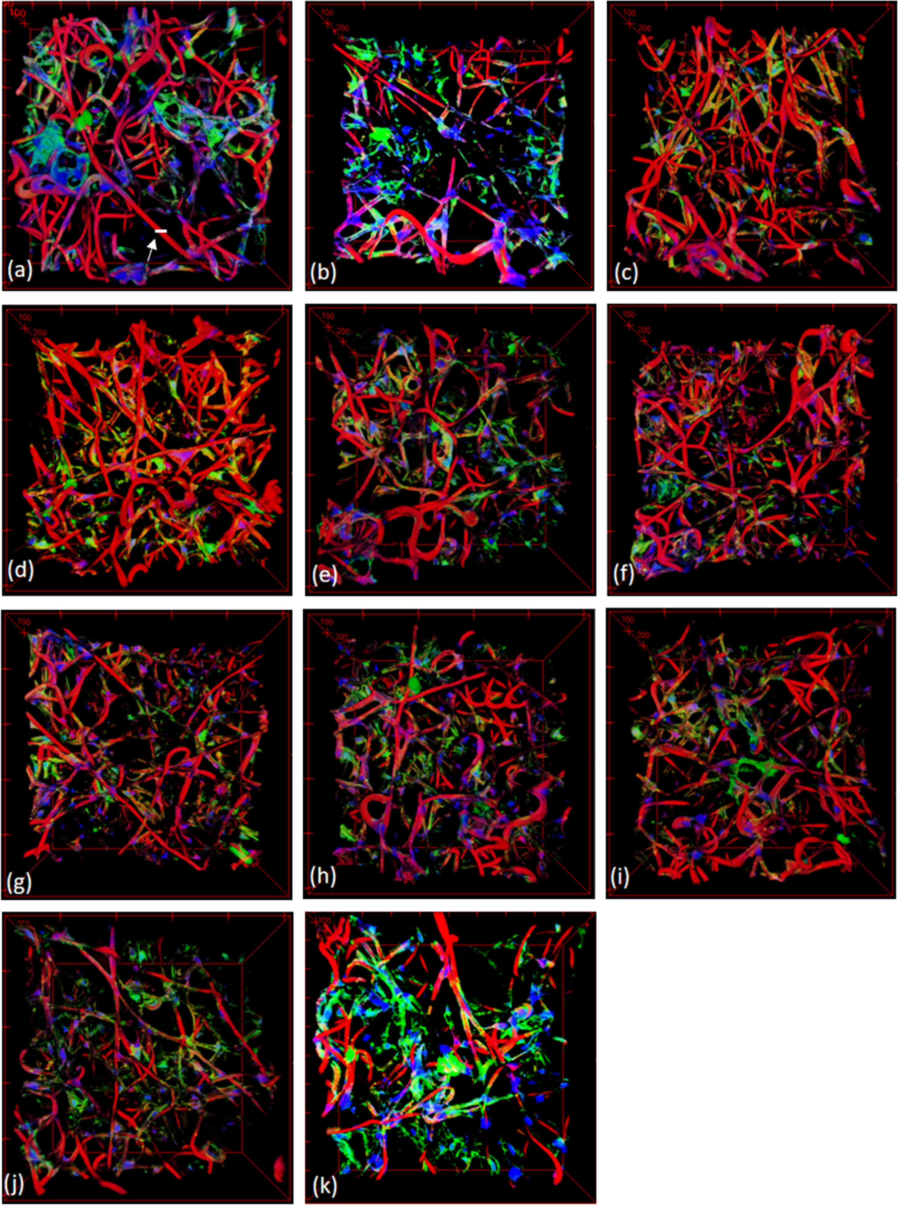
For the experiment, we have used 11 image volumes. We used a confocal microscope to obtain their original image volumes. Each voxel size of the 3D images was 1μm in the x-axis resolution, 1μm in the y-axis resolution, and 1.45μm in the z-axis resolution. The original image volumes were resampled so that the size of each voxel has the same resolution, but the number of the slices of an 3D image volume were adjusted so that it maintains the original image characteristics. The number of image slices in a 3D image volume was adjusted by multiplying the division of the z-resolution by the x-resolution to the original number of image slices for the purpose of image computation. Then, they were filtered with a Gaussian el to be resilient to noises. The volume visualized in Fig. 3(a) is of size 512×512×200, and that in Fig. 3(b) is of 512×512×322. For other cases shown in Fig. 3 (c)-(k), they were in a range between 200 and 350 in z-direction.
Fig. 3
3D confocal microscope images used for the experiment; the white scale bar designated by a white arrow in (a) is around 10μm.
After locating the upper left corner of a ω × ω × ω local widow Φ at the center of each template over all fibers in all 11 images, we calculated TPCF
Based on the calculated
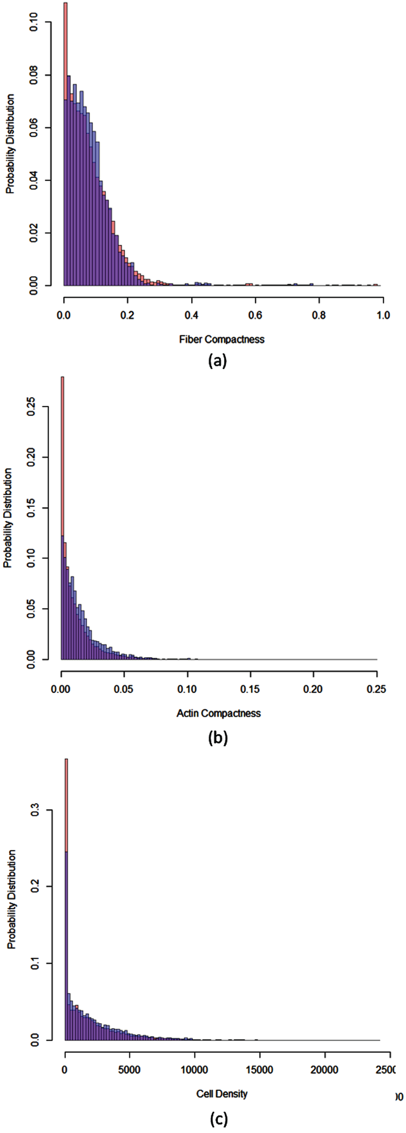
Figure 4 (a) shows the probability distribution of a fiber network compactness. Similarly, Fig. 4(b) is the probability distribution of actin compactness. Figure 4 (c) shows the probability distribution of cell density. In these probability distributions, the distribution over all templates (without considering if a template contains a CAB or not) in all 11 images is that in red. The distribution over templates containing CABs is in blue.
Fig. 4
Probability distributions. (a) The probability distribution of fiber network compactness; (b) the probability distribution of an actin distribution compactness; (c) the probability distribution of cell density. In these probability distributions, the distribution over all templates (without considering if a template contains a CAB or nor) is in red. The distribution over templates containing CABs is in blue.
In Fig. 4 (a), the distribution in red represents
In Fig. 4, the blue distribution covers the red distribution. This indicates that
Therefore, we conclude that
3Conclusion
In this research, we hypothesized that CABs would exist largely in the area with a high compactness of fibers, high compactness of actin, and high density of cells. For this purpose, we developed a compactness measure based on a two-point correlation function (TPCF). Next, we calculated the probability distribution of the compactness of a fiber network, the probability distribution of the compactness of an actin distribution, and the probability distribution of the density of cells in a local window. We then incorporated the famous Bayes theorem to those probability distributions. Finally, we verified the CAB’s existence with these processes.
We also proposed a local parameter that refers to the compactness of a local fiber network. Although the parameter is extensible over a whole fiber network in an image and its value is comparable to the value calculated from any other fiber network (i.e, which fiber network is more compact than the other), the parameter has a drawback to represent other statistical and topological meanings (e.g, centrality, clustering, of nodes in the graph representation of a fiber network). Thus, we plan to develop such a statistical and topological network parameter and then assess the statistical significance of the difference in comparison. We plan to develop a network parameter that contains more statistical and topological information and examine if this parameter brings meaningful improvements compared to the parameter used in this research through a statistical testing.
In the present study, we verified which type of regions contains CABs. We are still trying to explore why CABs exist in specific areas. Biologically, it seems that CABs are developed to attach cells to a fibrillar scaffold firmly. This biological observation needs to be verified mathematically as well.
4Method
4.1Two-point correlation function in 3-dimensional space
4.1.1Phase image
An image is composed of a certain number of discrete constituents. For example, 3-dimensional confocal microscopy image in Fig. 3 consists of 4 discrete constituents (i.e, fibers, actin, cells, and background black space). Each constituent defines a unique phase. Thus, the image in Fig. 3 has 4 phases. In this vein, we defined a phase image as a collection of discrete constituents. In other words, a phase image is partitioned into a certain number of disjointed phases. If a phase image I is composed of n phases from Pl to Pn, then
For each phase Pi, we define an indicator function for
(1)
4.1.2N-point Correlation Function (NPCF)
Suppose we have n points in a phase image I : x1, x2, …, xn. NPCF is defined as the probability that n points at positions x1, x2, …, xn land in the same phase Pi. It is the expectation of the product I(i) (x1) I(i) (x2) ⋯ I(i) (xn). Therefore, NPCF
(2)
4.1.2Two-point Correlation Function (TPCF)
As a specific case of the NPCF, the TPCF is defined as the probability that two points x1, x2 are in the phase i. Therefore, TPCF
(3)
If
Thus, in the case where a phase image is statistically homogenous and isotropic, TPCF
4.1.33D TPCF calculation
Kishore et al. [17] implemented a 2D version of TPCF for the segmentation with a 2D image. We extended it to a 3D version. A few modifications are required to implement 3D TPCF.
Given an L × M × N 3-dimensional phase image I, two-point correlation function
(4)
Let’s define
R(i) is normalized by an L × M × N matrix of ones in order to get probabilities
(5)
In order to get a homogeneous and isotropic TPCF, we need to sample circumferentially at a distance r from
(6)
4.1.4Example of TPCF distribution
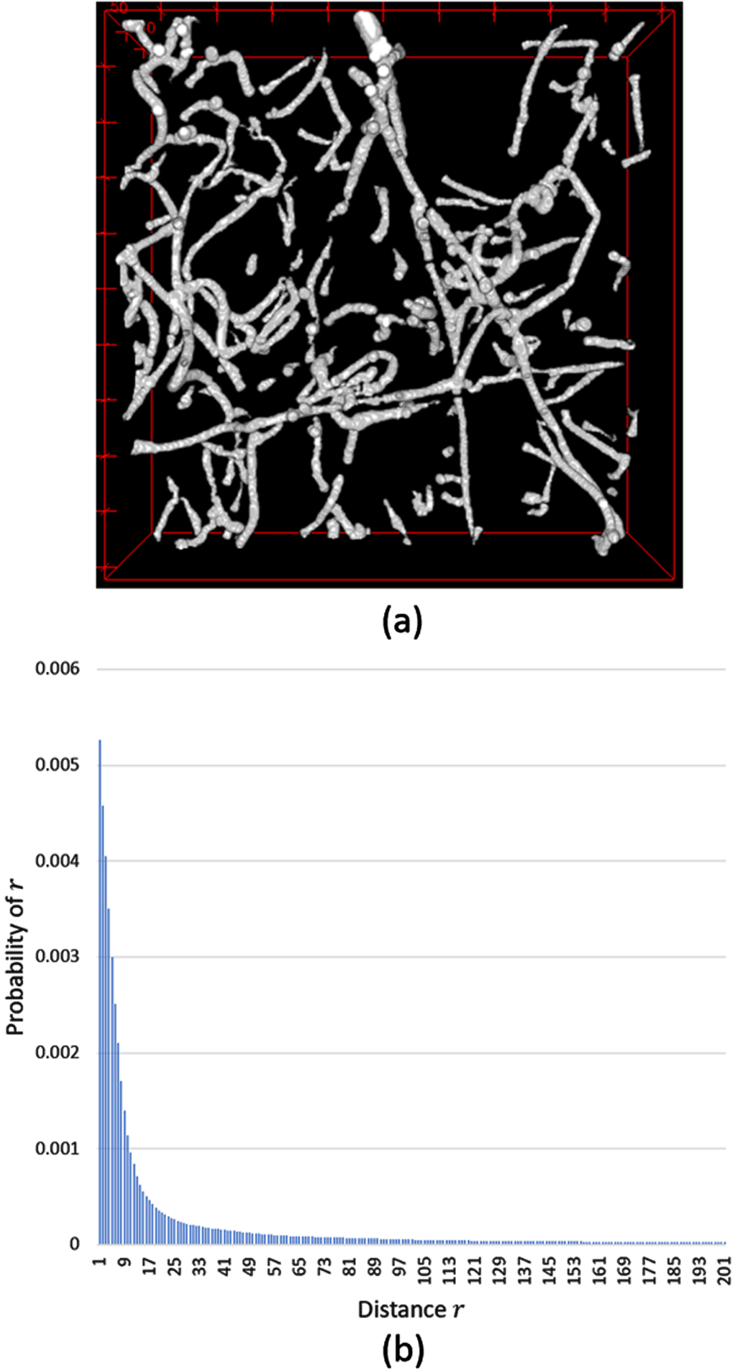
An example of the TPCF distribution according to the distance r is shown in Fig. 5 (b) for white area (a fiber network) in Fig. 5 (a). This distribution is calculated under the condition that, if we throw a needle of length r in the image Fig. 5 (a), both ends of the needle should be in that image space (that is, the needle cannot land outside the image). The distribution is the general shape of any fiber network (that is, it follows that the similar shape of poisson distribution has the shape parameter λ = 1).
Fig. 5
An example of the distribution of a two-point correlation function (TPCF) (a) The 3-dimensional image contains two phases (white phase: a fiber network, black phase: background). (b) The probability distribution of TPCF calculated from the image in (a).
4.2Compactness measure
We developed a measure that indicates the degree of compactness of a fiber network from a 3D confocal microscopy image containing fibers, actin, and cells. The fiber network in Fig. 5 (a) is represented in white phase.
Given an L × M × N 3-dimensional phase image I containing a fiber network in the white phase, assume that we throw a needle the length of r in the image I where 1 ≤ r ≤ max (L, M, N). If the probability that both ends of a needle have the length close to 1 and land over fibers is high, this indicates that the fiber network is compact. Based on this rationale and the fact that the shape of TPCF distribution over a fiber network has a similar shape of poisson distribution with the shape parameter λ = 1, we define the following compactness measure (mcompactness) as follows:
(7)
A as a normalization factor represents a case where an image of interest is filled with white phase. That is, the probability that both ends of a needle having any length land in the white phase is 1. This case is considered as the most compact one of a fiber network. Geometrically, mcompactness represents the portion of area enclosed by x-axis, y-axis, and the graph of
The measure mcompactness can be used to calculate the compactness of an actin distribution. If an actin distribution is wide and dense, the value of mcompactness produces a higher value.
4.3Bayes theorem
Hypothesis of CABs’ existence: It is more likely that CABs exist in an area of high compactness of a fiber network, high compactness of actin distribution, and high density of cells. (H.1)
In order to prove the above hypothesis, we applied the compactness measure (mcompactness) to a ω × ω × ω local region of interest (Φ) in the L × M × N 3-dimensional phase image I. The length ω of the local widow Φ is determined considering the diameter distribution of fibers so that the window Φ is not filled fully with a part of one fiber. In addition, the window Φ should not be filled fully with several fibers in the area having highly populated fibers. That is, the length ω should be determined for the window Φ to contain enough black phase.
We define
By the famous Bayes theorem, we have the following equations (8):
(8)
| Algorithm for Calculating Probability Distribution of Compactness and Density |
| For each image volume |
| For each fiber Fi |
| For each template tj in Fi |
| Put a local window Φ on tj |
| Compute the compactness (Cfn) of a fiber network in Φ |
| Compute the compactness (Cad) of an actin distribution in Φ |
| Compute the density (Dc) of cells in Φ |
| Store Cfn in a collection H(overall,Cfn) |
| Store Cad in a collection H(overall,Cad) |
| Store Dc in a collection H(overall,Dc) |
| If tj contains a CAB |
| Compute the compactness (Cfn) of a fiber network in Φ |
| Compute the compactness (Cad) of an actin distribution in Φ |
| Compute the density (Dc) of cells in Φ |
| Store Cfn in a collection H(CAB,Cfn) |
| Store Cad in a collection H(CAB,Cad) |
| Store Dc in a collection H(CAB,Dc) |
| End If |
| End For |
| Calculate two histograms: one from H(overall,Cfn), one from H(CAB,Cfn) and overlay them |
| Calculate two histograms: one from H(overall,Cad), one from H(CAB,Cad) and overlay them |
| Calculate two histograms: one from H(overall,Dc), one from H(CAB,Dc) and overlay them |
| End For |
| End For |
4.4Calculation of probability distribution of compactness and density
In this research, we hypothesized that CABs would exist largely in the area with a high compactness of fibers, high compactness of actin, and high density of cells. For this purpose, we developed a compactness measure based on a two-point correlation function (TPCF). Next, we calculated the probability distribution of the compactness of a fiber network, the probability distribution of the compactness of an actin distribution, and the probability distribution of the density of cells in a local window. We then incorporated the famous Bayes theorem to those probability distributions. Finally, we verified the CAB’s existence with these processes.
We defined a fiber as a set of templates in our previous algorithms [3] where a fiber is expressed as
(9)
The algorithm below shows the steps to compute the probability distribution over a collection of fiber network compactness, the probability distribution over a collection of actin compactness, and the probability distribution over a collection of cell densities.
References
[1] | Desiree J. , Park D. , Anghelina M. , Pecot T. , Machiraju R. , Xue R. , Lannutti J.J. , Thomas J. , Cole S.L. , Moldovan L. and Moldovan N.I. , Actin grips: Circular actin-rich cytoskeletal structures that mediate the wrapping of polymeric microfibers by endothelial cells, Biomaterials 52: ((2015) ), 395–406. |
[2] | Flusberg D.A. , Numaguchi Y. and Ingber D.E. , Cooperative control of Akt phosphorylation, bcl-2 expression, and apoptosis by cytoskeletal microfilaments and microtubules in capillary endothelial cells, Mol Biol Cell 12: ((2001) ), 3087–94. |
[3] | Park D.Y. , Jones D. , Moldovan N.I. , Machiraju R. , Pecot T. Robust detection and visualization of cytoskeletal structures in fibrillar scaffolds from 3-dimensional confocal images, In: IEEE Symposium on Biological Data Visualization, Atlanta, GA (2013), 25e32. |
[4] | Pecot T. , Singh S. , Caserta E. , Huang K. , Machiraju R. , Leone G. Non-parametric cell nuclei segmentation based on a tracking over depth from 3D fluorescence confocal images, Barcelona, Spain, IEEE Intl. Symposium on Biomedical Imaging (ISBI) (2012), |
[5] | Mosaliganti K. , Janoos F. , Sharp R. , Ridgway R. , Machiraju R. , Huang K. , Wenzel P. , deBruin A. , Leone G. and Saltz J. , Detection and visualization of surface-pockets to enable phenotyping studies, Medical Imaging IEEE Transactions 26: ((2007) ), 1283–1290 ISSN 0278-0062. |
[6] | Brown W.F. , Solid mixture permittivities, J. Chem. Phys 23: ((1955) ), 1514–1517. |
[7] | Frisch H.L. and Stillinger F.H. , Contribution to the statistical geometric basis of radiation scattering, –, J. Chem, Phys. 77: ((1982) ), 2071–2077. |
[8] | Torquato S. and Stell G. , Microstructure of two-phase random media, I. The-point probability functions, J. Chem, Phys 38: ((1982) ), 1982. |
[9] | Torquato S. and Stell G. , Microstructure of two-phase random media. III. The-point matrix probability functions for fully penetrable spheres, J. Chem Phys 79: ((1983) ), 1505–1510. |
[10] | Torquato S. and Stell G. , Microstructure of two-phase random media. IV. Expected surface area of a dispersion of penetrable spheres and its characteristic function, J. Chem Phys 80: ((1984) ), 878–880. |
[11] | Torquato S. and Stell G. , Microstructure of two-phase random media. V. The-point matrix probability functions for impenetrable spheres, J. Chem Phys 82: ((1985) ), 980–987. |
[12] | Ridgway R. , Irfanoglu O. , Machiraju R. , Huang K. Imagesegmentation with tensor-based classification of n-point correlationfunctions, Proceedings of the Microscopic Image Analysis withApplications in Biology (MIAAB) Workshop in MICCAI (2006). |
[13] | Janoos F. , Okan Irfanoglu M. , Mosaliganti K. , Machiraju R. , Huang K. , Wenzel P. , de Bruin A. , Leone G. , Multi-resolution image segmentation using the 2-point correlation functions, In Proceedings of IEEE International Symposium on Biomedical Imaging (2007), 300–303. |
[14] | Cooper L.A.D. , Saltz J.H. , Machiraju R. , Huang K. Two-pointcorrelation as a feature for histology images: feature spacestructure and correlation updating,Mathematical Methods in Bioimage Analysis Workshop, 23rd IEEEConference on Computer Vision and Pattern Recognition, SanFrancisco, CA (2010), 79–86. |
[15] | Sahai H. , Bayes’ theorem: some examples in computer-aided medical diagnosis, Int. J. Math. Educ. Sci. Technol 23: (2) ((1992) ), 257–266. |
[16] | De Silva N.T. and Jayamanne D. , Computer-aided medical diagnosis using bayesian classifier –decision support system for medical diagnosis, Int. J. Multidisciplinary Studies (IJMS) 3: (2) ((2016) ). |
[17] | Mosaliganti K. , Janoos F. , Sharp R. , Ridgway R. , Machiraju R. , Huang K. , Wenzel P. , deBruin A. , Leone G. and Saltz J. , Detection and visualization of surface-pockets to enable phenotyping studies, Medical Imaging IEEE Transactions 26: ((2007) ), 1283–1290. ISSN 0278-0062. |

