
Personalized statistical learning algorithms to improve the early detection of cancer using longitudinal biomarkers
Abstract
BACKGROUND:
Patients undergoing screening for early detection of cancer have serial biomarker measurements that are not traditionally being incorporated into decision making when evaluating biomarkers.
OBJECTIVE:
We discuss statistical learning algorithms that have the ability to learn from patient history to make personalized decision rules to improve the early detection of cancer. These artificial intelligence algorithms are able to learn in real time from data collected on the patient to identify changes in the patient that could signal asymptomatic cancer.
METHODS:
We discuss the parametric empirical Bayes (PEB) algorithm for a single biomarker and a Bayesian screening algorithm for multiple biomarkers.
RESULTS:
We provide tools to implement these algorithms and discuss their clinical utility for the early detection of hepatocellular carcinoma (HCC). The PEB algorithm is a robust, easily implemented algorithm for defining patient specific thresholds that can improve the patient-level sensitivity of a biomarker in many settings, including HCC. The fully Bayesian algorithm, while more complex, can accommodate multiple biomarkers and further improve the clinical utility of the algorithms.
CONCLUSIONS:
These algorithms could be used in many clinical settings and we aim to guide the reader on how these algorithms may improve the detection performance of their biomarkers.
1.Introduction
Artificial intelligence (AI) aims to create algorithms that have the ability to learn from large amounts of data and then used to make predictions about future states. This idea can be very useful in the context of developing biomarkers for early detection of cancer. Our goal is to understand the biomarker behavior in the early pre-clinical phase and hence learn how to differentiate between two types of patients at each cancer screening visit. Those who have asymptomatic cancer, which will be clinically diagnosed in the near future, compared to those who will remain cancer free at their next screening visit. Most AI algorithms that have been published to date have involved large databases in which an algorithm, such as a convolutional neural network, was used to learn the relevant information for predictions. However, the term AI could also be used to refer to more “traditional” statistical methods that in real time, learn from updated patient-level biomarker data over time to make new predictions about patient risk. These are the type of algorithms we will discuss here. There are two statistical approaches that have gained the most traction in early detection of cancer using longitudinal biomarker trajectories.
The parametric empirical Bayes (PEB) algorithm was first proposed by McIntosh and Urban using serial CA125 for ovarian cancer screening[1]. The PEB algorithm for a single biomarker is an AI algorithm in that instead of using the same biomarker threshold for each patient at every screening visit, the algorithm defines a patient specific threshold that updates at each screening visit to take into account the screening history of the patient. The threshold is a weighted average of the mean biomarker level in the population (based on a hierarchical model for the biomarker in cancer free patients in the target screening population) and the patients average biomarker level to date. At each screening visit, the current biomarker level is compared to the patient’s individualized threshold with the goal being to detect changes in biomarker level that are significant deviations for that patient in the context of their screening history. The distinctive AI features here are the personalized decision rule based on adaptive learning over time as data accumulates.
Skates et al. have proposed a fully Bayesian approach for early detection of cancer using a single biomarker, again in the context of ovarian cancer screening with CA125[2]. The fully Bayesian algorithm uses the posterior risk of cancer to make screening decisions at each visit. The posterior risk estimate is updated at each screening visit to take into account the longitudinal trajectory of the biomarker to date. The posterior risk is the ratio of two probabilities: probability the patient has cancer, given the biomarker trajectory, and the probability the patient remains cancer-free, given the biomarker trajectory. This risk estimate can then be used to make decisions about whether the patient has undetected cancer and should undergo further clinical work-up. The risk of ovarian cancer algorithm (ROCA) is the only longitudinal biomarker algorithm that has been studied prospectively[3, 4], however the added sensitivity provided by the algorithm when applied to longitudinal CA125 measurements demonstrates that this approach should be actively studied in other cancer screening settings.
More recently, these algorithms have been generalized to allow for screening with multiple biomarkers. It is unlikely that a single biomarker will have sufficient utility for early detection given the heterogenous nature of cancer and the risk settings from which it arises. Therefore, algorithms that allow for screening with multiple longitudinal biomarkers are necessary and an area of active research interest for us. Tayob et al. have proposed a generalized fully Bayesian screening algorithm where the posterior risk estimate is conditional on the longitudinal trajectory of multiple (potentially correlated) biomarkers[5]. This generalization requires additional algorithm complexity but increases the potential utility in changing clinical practice to improve early detection of cancer.
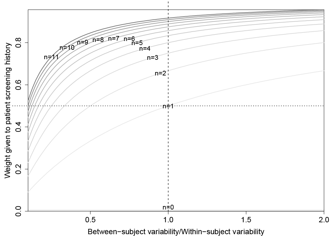
Figure 1.
Weighting of patient sample average in the personalized threshold defined by the parametric empirical Bayes algorithm. The weight is a function of the number of prior screens (
For a researcher with a novel biomarker, or biomarker panel, that has shown promise in early validation studies for differentiating clinically diagnosed cancer cases, particularly early-stage cancers, from cancer free patients in Phase 2 studies using EDRN 5-Phase terminology, the next step is often to study the biomarker(s) ability to detect pre-clinical disease, i.e. a Phase 3 study[6]. These evaluations require a longitudinal cohort study with an associated biospecimen database where the biomarker(s) can be retrospectively evaluated. When there is a serial blood collection in the cohort a researcher could ask the question, is it the absolute level of the biomarker or the trajectory of the biomarker that contains important information about cancer onset. If it is the case that the trajectory has key information, a biomarker algorithm that incorporates the longitudinal history should be considered to gain additional sensitivity for early detection. In this paper, we aim to guide the researcher on how these algorithms could be used to improve the detection performance of their biomarkers.
We start by reviewing longitudinal algorithms for a single biomarker. We introduce an online tool that we have created to assist in researchers in evaluating the PEB algorithm when applied to their biomarker of interest. We then discuss the longitudinal algorithm for multiple biomarkers. For all these algorithms, we discuss the properties of these algorithms that could guide researchers to better understand their utility in different contexts through both simulation studies and real data analyses. In this paper, our data analyses have focused on the early detection of hepatocellular carcinoma (HCC) where we have been able to evaluate these algorithms. In the discussion we review some other settings where these algorithms could be studied.
2.Parametric empirical Bayes algorithm
A key advantage of the PEB algorithm for a single biomarker is that it only requires specifying a model for the biomarker trajectory in the cancer free target screening population. Longitudinal cohort studies typically have a larger number of patients that are within the target screening population but remain cancer free for the duration of the study. These are patients for whom we have the most data to estimate the trajectory of a screening biomarker. We use a hierarchical model structure to allow each patient to have its own mean biomarker levels in the absence of cancer. This flexibility allows our model to accommodate the biomarker heterogeneity we observe in the screening populations. Clinical covariates could also be included at this stage as either time-varying or time-invariant to explain the additional heterogeneity we may observe in the biomarker levels that are unrelated to the onset of cancer. The algorithm will then identify significant deviations from expected behavior to select patients that we suspect have asymptomatic cancer and should receive additional follow-up testing, which may lead to a cancer diagnosis.
Without loss of generality, we assume the biomarker being evaluated increases with cancer onset. The methods can be easily adapted to biomarkers that decrease with cancer onset. Suppose we have a patient who has completed
The estimate of the expected biomarker levels is a weighted average of the population mean biomarker levels in the cancer-free target screening population and the sample average of prior
The PEB algorithm assumes that the biomarkers are normally distributed but for continuous biomarkers, a transformation is assured and since screening rules are invariant to monotonic transformations, we don’t lose generality based on this assumption. In practice the methodology is robust to deviations from normality by estimating the specificity without any distributional assumptions. To demonstrate this, we conducted a simulation study where we generated biomarkers from different distributions and compared the discriminatory performance of the PEB algorithm and a fixed threshold decision rule.
Standard definitions for sensitivity and specificity in receiver operating characteristic (ROC) curves are based on single time point evaluation of the biomarker. In our setting, where we have serial screening evaluations in the cohort, we have modified these definitions. We estimated the false positive rate (FPR) at the screening level, defined as the proportion of positive results among all the screenings conducted in the cancer-free patients within the cohort. This accounted for all false positive results in the screening program. The screening-level specificity was defined as 1-FPR. We estimated the true positive rate or sensitivity at the patient-level, defined as the proportion of cancer cases with at least one positive screening during the pre-diagnostic period.
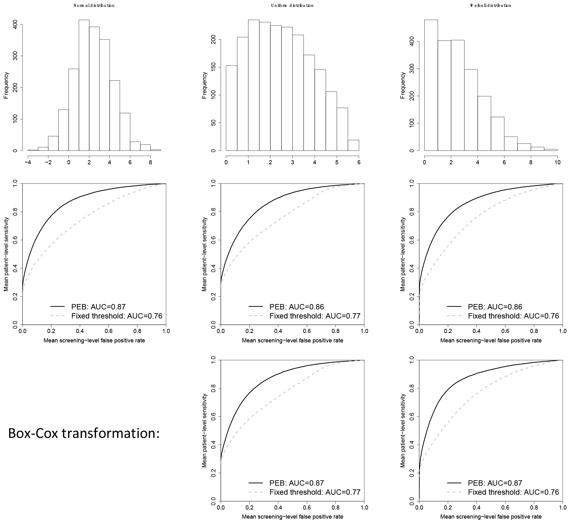
Our simulation study assumed we have a cohort of 400 patients that have been followed for every 6 months for up to 5 years, with 50 out of 400 patients developing cancer during follow-up. The biomarker is assumed to be stable prior to cancer onset and thereafter increases linearly but only in 50% of patients. For the remainder, the biomarker is non-informative for cancer onset and remains stable even after onset of cancer. The maximum preclinical duration was assumed to be 2 years and the average preclinical duration was set at 1 year. Additional details on the simulation study design can be found in Tayob et al. (2017)[5]. We generated 500 cohort studies, evaluated the PEB algorithm within each cohort and thereafter summarized the results observed across the studies to obtain the mean patient-level sensitivity and mean screening-level FPR. We considered three possible distributions for the biomarker: (1) normal distribution, (2) uniform distribution and (3) Weibull distribution. We applied the PEB algorithm without any transformation and after a Box-Cox transformation to the biomarker. In Fig. 2, we observe that for both the uniform distribution that has no distinct mode, or the Weibull distribution that has a heavy tail on the right, the PEB algorithm has improved discriminatory performance even without a transformation to normality. The area under the ROC curve (AUC) for the PEB algorithm is 0.87 when the biomarker is normally distributed and 0.86 for the uniform and Weibull distributions. The AUC improves to 0.87 for both distributions after a Box-Cox transformation of the data. Hence, the PEB algorithm is robust to the normality assumptions used in the algorithm development.
Figure 2.
Distribution of the biomarker in patients that remain cancer-free in the cohort (top row); mean receiver operating curves (ROC) for the parametric empirical Bayes algorithm (PEB), applied to the biomarker without any transformation, and a fixed threshold decision rule (middle row); ROC curve for the PEB algorithm after a Box-Cox transformation of the biomarker and a fixed threshold decision rule (bottom row). AUC: area under the ROC curve.
Another advantage of the PEB algorithm is the ability to learn from prior false positive screening. Patients with stable biomarker trajectories that are consistently higher than average, are identified and no longer indicated to have positive screening after a few false positives. A fixed threshold rule does not have this ability to adapt and will continue to indicate positive screens in patients with biomarker values that are persistently higher than the fixed threshold value even when the biomarker trajectories are stable. Each false positive result leads to further testing, which can be expensive and may lead to complications and anxiety. The ability to reduce the number of false positive results within each patient is a direct advantage of a personalized decision rule based on adaptive learning over time as patient screening history accumulates.
Figure 3.
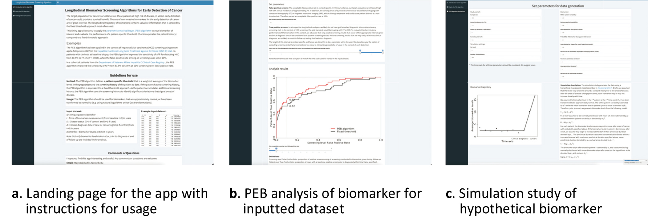
Parametric empirical Bayes (PEB) algorithm app (https://rconnect.dfci.harvard.edu/PEBalgorithm/).
2.1Steps to implement the PEB algorithm
1. Consider if a transformation of the biomarker is required.
a. Plot a histogram of the biomarker in patients that have not developed cancer.
b. Compare to histogram of the transformed biomarker (e.g. log transformation or a Box-Cox transformation with tuning parameter estimated using only patients that have not developed cancer)
2. Using only patients that have not developed cancer, fit a random intercept mixed model. If clinical covariates are being included, they can be included at this stage as either time-varying or time-invariant variables in the mixed model. Model estimation can be done in standard statistical software (e.g. lme in R, proc mixed in SAS).
3. Three parameter estimates are then extracted from this model.
4. If
And we define
5. The PEB rule is then:
while the fixed threshold decision rule is:
6.
While the steps of the algorithm are relatively simple to implement for those with programming skills, to further increase the utility of the PEB algorithm, we have developed a web-based Shiny App that allows a user to implement the PEB algorithm for their biomarker and explore the performance of the algorithm in different scenarios using simulations.
2.2Shiny App for PEB algorithm
The PEB algorithm app (https://rconnect.dfci.harvard. edu/PEBalgorithm/) allows a user to apply the PEB algorithm to a biomarker and evaluate the improvement in early detection performance when incorporating screening history compared to a single timepoint evaluation of the biomarker. The landing page, shown in Fig. 3a, includes guidelines on to use the app and an example of the data structure required for input.
The PEB algorithm is applied in longitudinal cohort datasets and therefore the input data requires both a subject identifier (ID) and a measurement time of the biomarker (
Once the analysis dataset has been assembled, it can be uploaded for analysis (Fig. 3b). The user then needs to select an acceptable false positive rate. The acceptable false positive rate is context specific. For example, in HCC screening the target population are those with cirrhosis of the liver that have annual incidences of approximately 1–3% and the consequences of a positive screen would be additional imaging with computed tomography (CT) or magnetic resonance imaging (MRI)[7]. Therefore, in HCC we set an acceptable false positive rate at 10%. Next, the user needs to define the pre-diagnostic period that is of interest when estimating the patient-level sensitivity. In retrospective longitudinal analyses, we likely do not have gold standard diagnostic information at every screening visit. In the context of HCC screening, the gold standard would be imaging with CT or MRI. To evaluate the discriminatory performance of the biomarker in this context, we advocate that only positive screening results that occur within appropriate intervals prior to clinical diagnosis should be considered true positive screening results. Positive screening results that are very early, relative to clinical diagnosis, are unlikely to result in follow-up testing that leads to a diagnosis. The app also allows the user the option of excluding screening tests that are considered too close to clinical diagnosis to be of value in the context of early detection. These are screening results that are unlikely to introduce a stage shift for the cancer diagnosed.
Lastly, the app allows a user to study the improvements in early detection performance when incorporating screening history, compared to a fixed threshold decision rule, of a hypothetical biomarker via a simulation study (Fig. 3c). Here the user can generate data from a hierarchical changepoint model described in Tayob et al.[5] and then evaluate the improvement of the PEB algorithm. The user can vary factors such as screening interval, within- and between-patient variability, preclinical duration, and biomarker slope after onset to examine their effect on the PEB algorithm performance.
3.Multivariate fully Bayesian screening algorithm
While the PEB algorithm is a useful and robust algorithm for incorporating patient history to obtain personalized, adaptive decision rules for screening, a key disadvantage of the algorithm is that it can only be used for a single biomarker. One approach to using the PEB algorithm with a biomarker panel is to first define a rule to combine the multiple biomarkers into a single continuous score (e.g. using logistic regression or a Cox proportional hazards model). The PEB can then be applied to the score with the assumption that the trajectory of the score contains the key information about onset of cancer. A weakness of this approach is that it assumes the biomarkers in the panel have a fixed relationship with each other that does not change over time and does not incorporate any variability in the relationship between the biomarkers in different patients.
We have developed a Bayesian model-based algorithm that utilizes the patient trajectory of multiple biomarkers to obtain a personalized screening decision rule based on the posterior risk estimate[5]. When we extended the algorithms to multiple biomarkers, we could no longer restrict algorithm development to only data from patients that have not developed cancer. Instead, we require a longitudinal training cohort, that includes patients that have developed cancer during the study and those that remain cancer-free, and therein we estimate the parameters of a model that describes the joint pre-clinical trajectory of the multiple biomarkers.
The personalized decision rule of the fully Bayesian algorithm is based on the posterior risk estimate after inputting the patient’s screening history to date on the multiple biomarkers. The posterior risk of cancer is the ratio of the probability that the patient has cancer knowing the biomarker trajectories that we have observed to date, to the probability the patient remains cancer-free. We use an application of Bayes rule to separate out this risk ratio into the product of two probability ratios that are easier to estimate. The first include the probabilities of observing the biomarker trajectory for that patient if a patient has cancer or if they remain cancer free, and the second ratio is the risk of having cancer or remaining cancer free regardless of the biomarker trajectories observed. We can represent this in mathematical notation as follows:
The probabilities of observing the biomarker trajectories if a patient has cancer or if they remain cancer free are estimated after specifying a model for the biomarker trajectory in those that remain cancer free and those that develop cancer. This demonstrates the additional complexity over the PEB algorithm, which only required a model for the biomarker trajectory in those that remained cancer free, when we generalize to multiple biomarkers in screening.
Figure 4.
Biomarker model structure assumed in the generalized fully Bayesian algorithm for screening with multiple biomarkers.
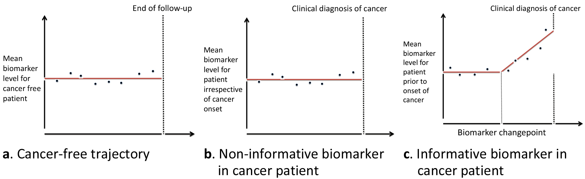
To maintain consistency, we assume the same model structure for the biomarker trajectories in those that remain cancer free. For each biomarker, we assume it has a stable flat trajectory prior to the onset of cancer using a hierarchical model structure (Fig. 4a). In those that develop cancer, we allow for two possible biomarker trajectories after onset. The first is that an individual biomarker is non-informative in that patient and remains stable after onset of cancer until clinical diagnosis (Fig. 4b). The second possible trajectory is that after onset of cancer, we observe a changepoint in the biomarker trajectory and the biomarker starts increasing linearly (Fig. 4c). Biomarkers that decrease after onset can easily be accommodated in the framework of the algorithm. Again, we assume a hierarchical model structure for each biomarker with each patient having its own mean biomarker level prior to onset, changepoint time, and rate of change after onset of cancer.
We connect the multiple biomarkers through the parameters that indicate whether we observed a changepoint for each biomarker by specifying a Markov random field (MRF) prior distribution on these parameters. Whether or not we observe a changepoint is a key component of identifying early onset of cancer and hence we focused on that component of the joint model to connect the biomarkers. The MRF prior assumes that the probability of observing a changepoint for any biomarker depends on how many changepoints were observed for other biomarkers in that patient. This allowed us to borrow information across biomarkers and defined a dependence structure helpful for detecting borderline changepoints. Additional details of the model specified in the fully Bayesian screening algorithm are included in the supplementary files provided.
The fully Bayesian screening algorithm is flexible and allows for biomarkers that are measured at different intervals and accommodates missing data. The posterior risk calculation used all the biomarker accumulated to date on the patient to make an updated prediction of risk of cancer. Also, by including model structure for the biomarkers during the preclinical period, we incorporate additional prior knowledge of the biomarkers when it’s available and increase the power of the algorithm to detect changepoints in biomarker trajectory that signal the onset of cancer. A disadvantage of the approach is that we require a sufficiently large longitudinal training cohort to estimate the model parameters, especially those related to the changepoints that occur during the preclinical period. This can be a limitation for the application of the algorithm for novel biomarkers in disease settings where appropriate biospecimen repositories are limited.
3.1Steps to implement the multiple biomarker screening algorithm
We are currently planning an update to the Shiny app (Fig. 3) to implement the fully Bayesian algorithm, but this is not a straightforward inclusion given the complexity of the multiple biomarker screening algorithm. At this time, researchers interested in implementing the algorithm for their biomarker panel can use the R code provided at https://github.com/ntayob/Multivariate-Fully-Bayesian-Longitudinal-Biomarker-Screening-Algorithm. The code provided allows the user to either apply the algorithm and evaluate its performance in an independent validation cohort or modify it as necessary for those with a background in Bayesian model fitting. We have provided example training and validation cohorts for the user to experiment with as they are learning to implement the algorithm.
A few key points, the fully Bayesian algorithm has underlying distributional assumptions for the joint biomarker model used. These need to be assessed for validity prior to implementing the algorithm in the validation cohort. As with the PEB algorithm, a transformation of the data to approximate normality improves the stability of the algorithm. The algorithm uses a Markov chain Monte Carlo algorithm to estimate the model parameters. We have found that running two chains with different starting points, removing the burn-in and thinning the chains to reduce autocorrelation were necessary. These steps have been implemented in the code provided and the user can modify them as necessary. We have also provided code to generate standard Bayesian diagnostic tools, such as trace plots and the Gelman-Rubin statistic to assess convergence of the chains.
The prior distributions specified for model parameters related to the biomarker changepoint, such as the MRF prior, require sensitivity analyses to ensure the results of the algorithm are robust to the prior distribution assumptions. These parameters are usually estimated with the least amount of data and therefore rely more on the model structure provided. It is important to understand how sensitive the conclusions of the algorithm are to the choice of these parameters. In our analysis we have found with cohorts of
Figure 5.
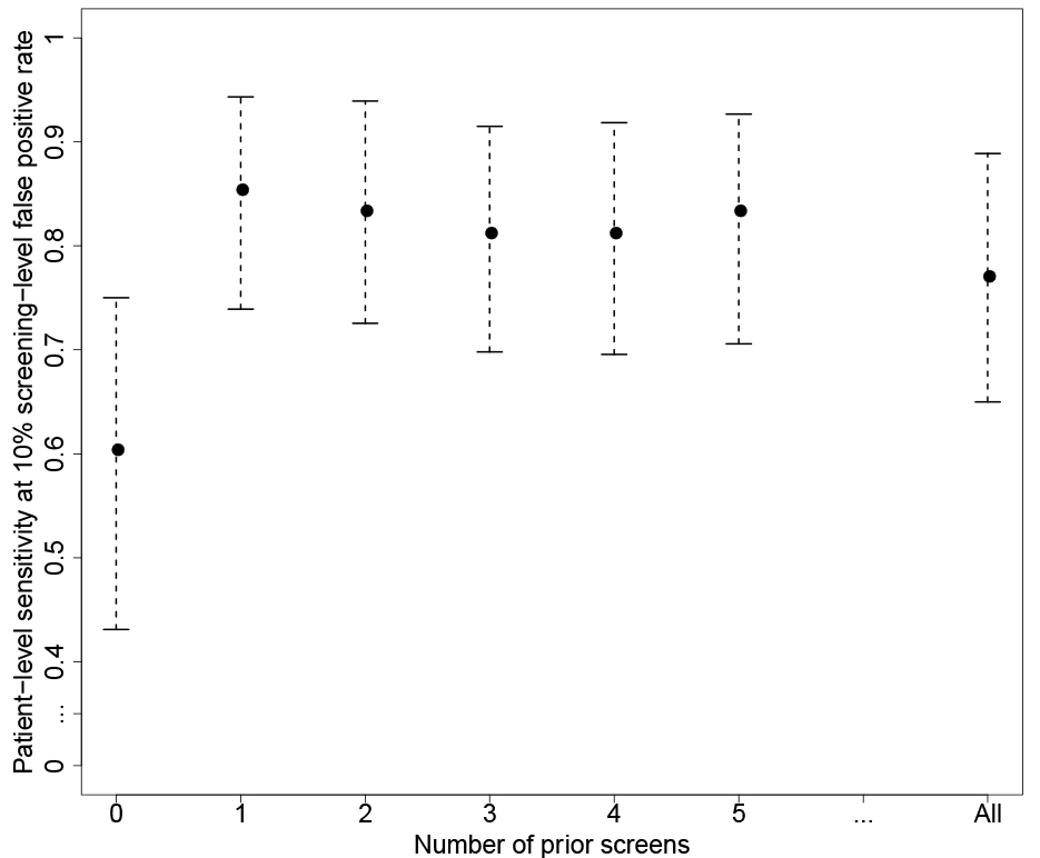
Patient-level sensitivity corresponding to 10% screening-level false positive rate (and associated 95% bootstrap confidence intervals) for varying number of prior screening results used in the parametric empirical Bayes algorithm applied to the patients with cirrhosis at baseline in the HALT-C trial.
4.Implementation of algorithms in the HALT-C trial
The Hepatitis C Antiviral Long-term Treatment against Cirrhosis (HALT-C) trial enrolled patients with either active hepatitis and either cirrhosis or advanced fibrosis at baseline[8]. The trial evaluated if long-term low dose pegylated interferon was a safe, efficacious treatment in preventing fibrosis progression and other clinical outcomes, including HCC, and found no reduction in the incidence of HCC compared with no treatment. Among the 427 patients with cirrhosis at baseline, 48 developed HCC during the follow-up period. We excluded 18 patients that did not develop HCC but had less than one year of follow-up to rule out undiagnosed HCC. Among the 621 patients with advanced fibrosis at baseline, 40 developed HCC during the follow-up period and 23 patients did not develop HCC but had less than one year of follow-up and were excluded. Patients enrolled in the trial had extensive follow-up, which makes this study a valuable resource for understanding HCC screening using longitudinal biomarkers. The median follow-up in the cohort was 76.4 months. We have studied the performance of the algorithms in both those with cirrhosis and advanced fibrosis at baseline but since current guidelines recommend HCC screening in those with cirrhosis [9], we discuss the performance of the algorithms in those with cirrhosis at baseline here.
Longitudinal algorithms are of great interest in HCC screening for a few key reasons. The American Association for the Study of Liver Diseases (AASLD) Guidelines recommend ultrasonography screening with or without serum
Blood-based biomarkers are a promising tool for more effective, widespread HCC screening. Des-
More recently, we have focused on applying the proposed algorithms to AFP and DCP measurements in the HALT-C trial and have demonstrated their potential clinical utility[5, 17]. Note that AFP-L3 was not evaluated in these analyses since the study included only measurements from an older version of the assay that differs from the FDA approved assay. Patients in the HALT-C trial had AFP levels measured at a local laboratory every three months during the first 42 months post randomization and every six months thereafter in the extended phase of the study. DCP was measured after the completion of the trial within the biomarker repository created that included specimens collected every three months during the first 42 months of the study. As noted earlier, at 10% FPR is considered acceptable in HCC screening due to the high-risk target population – reported specificity of AFP in clinical practice is 90%.[11]. We had previously reported that the patient-level sensitivity of the PEB algorithm applied to AFP was 77.1% at the 10% screening-level FPR, a significant improvement over AFP at a fixed threshold whose patient-level sensitivity at the 10% screening-level FPR was 60.4%[17].
In Fig. 5, we explored the performance of the PEB algorithm as we vary the maximum number of prior screening values included. When we don’t include any prior screenings, the PEB algorithm is equivalent to a fixed threshold decision rule for AFP. With just a single prior screening included, we observe an improvement in the patient-level sensitivity comparable to if we set no limits on the number of prior screening values. Thereafter, the estimates are stable for increasing the number of prior screening results included. This is likely due to the fact that in this cohort, the within-patient variance of AFP is 0.19 while the between-patient variance is 0.85. Therefore, of the total variance we observe in AFP, within-patient variance is less than 20% and having additional prior AFP screens after the first to estimate the patient mean does not further improve the performance of the PEB algorithm. In other settings this may not be the case and the PEB algorithm is relatively simple to implement when including all the prior screening results when required.
Table 1
Cross-validated patient-level sensitivity at 10% screening-level false positive rate in the HALT-C trial for the fully Bayesian algorithm applied to AFP and DCP, the parametric empirical Bayes algorithm applied to either AFP or DCP and a fixed threshold decision rule applied to either AFP or DCP
| Time period | Biomarker | Fully Bayesian algorithm | Parametric empirical Bayes algorithm | Fixed threshold |
|---|---|---|---|---|
| Any time prior to clinical diagnosis | log(AFP) | 89.5% | 77.0% | 60.4% |
| log(DCP | 60.5% | 56.2% | ||
| 2-years prior to clinical diagnosis | log(AFP) | 60.5% | 60.0% | 50.0% |
| log(DCP | 58.3% | 56.2% | ||
| 1-year prior to clinical diagnosis | log(AFP) | 59.5% | 57.0% | 46.8% |
| log(DCP | 56.5% | 50.0% |
We used 10-fold cross validation to compare the fully Bayesian screening algorithm applied to AFP and DCP jointly to the PEB algorithm applied to AFP or DCP alone and a fixed threshold approach for each. In Table 1, we observe that a joint screening approach with the two biomarkers combined resulted in increased patient-level sensitivity at 10% screening-level false positive rate of 89.5% compared to the PEB algorithm applied to either AFP or DCP alone (77.0% and 60.5%, respectively) at any time prior to HCC diagnosis[5]. The PEB algorithm itself had improved patient-level sensitivity compared to a decision rule based on a fixed threshold for either biomarker with larger gains observed for AFP compared to DCP. This is likely due to the increased variability observed in DCP, where the within-patient variance of DCP was 1.37 while the between-patient variance is 0.71. Therefore, 66% of the total variance we observe in DCP is within-patient variance.
The improvement in patient-level sensitivity was diminished in the 1-year and 2-year intervals prior to clinical diagnosis for HCC. It is not clear that this is a weakness of the algorithm or specifically due to the HALT-C study design wherein DCP was only measured in the first 42 months post randomization and therefore we do not have DCP measured at screening times leading up to clinical diagnosis for all the patients diagnosed in the extended phase of the study. While our fully Bayesian algorithm is flexible enough to accommodate this type of differential measurement of the biomarkers, it then becomes difficult to determine if the lack of improvement when adding longitudinal DCP to longitudinal AFP during key windows is due to the algorithm itself or insufficient data and further examination of these algorithms in other cohorts is required to understand the clinical utility of these multiple longitudinal biomarker screening algorithms.
5.Discussion
The use of biomarkers for early detection of cancer is an area of active research to improve patient outcomes across multiple cancer types. In this paper, we discussed longitudinal biomarker screening algorithms that could be used to further improve the early detection performance of these biomarkers by utilizing a personalized decision rule based on adaptive learning as patient data accumulates.
We have focused on the development of algorithms for early detection of HCC using serum biomarkers here, but these statistical learning algorithms are generally applicable across many different settings and these algorithms could be used for different types of biomarkers. For example, in breast cancer screening patients undergo biennial mammography for women aged 50 to 74 years([18]. There has also been work done to quantify the mammography images using radiomics features extracted[19]. These radiomics features could be used as biomarkers in a longitudinal algorithm to incorporate patient screening history and identify changes in the image that could signal onset of cancer.
The algorithms are not specific to the early detection of cancer but can also be used for updating risk prediction estimates, and for monitoring patients for cancer recurrence. The key principle is that we are able to measure a biomarker (or biomarker panel) longitudinally and significant deviation in the biomarker(s) signal a change in patient health status that is of interest. While the multiple biomarker algorithms do have greater complexity compared to the single biomarker algorithms, the incorporation of additional information to capture disease heterogeneity is likely to produce the greatest improvement in patient outcomes.
Author contributions
Both authors contributed to the conception, interpretation or analysis of data, preparation of the manuscript and revision for important intellectual content.
Supplementary data
The supplementary files are available to download from http://dx.doi.org/10.3233/CBM-210307.
Acknowledgments
Dr. Tayob is supported in part by NIH R01CA230503 and U24CA230144. Dr. Feng is supported in part by NIH R01CA230503, U24CA230144 and U24CA086368.
The content is solely the responsibility of the authors and does not necessarily represent the official views of the National Institutes of Health. The funding agency had no role in design and conduct of the study; collection, management, analysis, and interpretation of the data; or preparation of the manuscript.
References
[1] | M.W. McIntosh and N. Urban, A parametric empirical Bayes method for cancer screening using longitudinal observations of a biomarker, Biostatistics 4: (1) ((2003) ), 27–40. doi: 10.1093/biostatistics/4.1.27. |
[2] | S.J. Skates, D.K. Pauler and I.J. Jacobs, Screening based on the risk of cancer calculation from Bayesian hierarchical changepoint and mixture models of longitudinal markers, J Am Stat Assoc 96: (454) ((2001) ), 429–439. http://www.jstor.org/stable/2670281. |
[3] | U. Menon, S.J. Skates, S. Lewis et al., Prospective study using the risk of ovarian cancer algorithm to screen for ovarian cancer, J Clin Oncol 23: (31) ((2005) ), 7919–7926. doi: 10.1200/JCO.2005.01.6642. |
[4] | S.J. Skates, Ovarian cancer screening: Development of the risk of ovarian cancer algorithm (ROCA) and ROCA screening trials, Int J Gynecol Cancer 22: (Suppl 1) ((2012) ), S24–6. doi: 10.1097/IGC.0b013e318256488a. |
[5] | N. Tayob, F. Stingo, K.-A. Do, A.S.F. Lok and Z. Feng, A Bayesian screening approach for hepatocellular carcinoma using multiple longitudinal biomarkers, Biometrics (May (2017) ), 1–11. doi: 10.1111/biom.12717. |
[6] | M.S. Pepe, R. Etzioni, Z. Feng et al., Phases of biomarker development for early detection of cancer, J Natl Cancer Inst 93: (14) ((2001) ), 1054–1061. http://jnci.oxfordjournals.org/content/93/14/1054.short. |
[7] | A.G. Singal, Y. Hoshida, D.J. Pinato et al., International liver cancer association (ILCA) white paper on biomarker development for hepatocellular carcinoma, Gastroenterology (March (2021) ). doi: 10.1053/j.gastro.2021.01.233. |
[8] | A.S. Lok, J.E. Everhart, E.C. Wright et al., Maintenance peginterferon therapy and other factors associated with hepatocellular carcinoma in patients with advanced hepatitis {C}, Gastroenterology 140: (3) ((2011) ), 840–849. |
[9] | J.K. Heimbach, L.M. Kulik, R.S. Finn et al., AASLD guidelines for the treatment of hepatocellular carcinoma, Hepatology 67: (1) ((2018) ), 358–380. doi: 10.1002/hep.29086. |
[10] | A.G. Singal, H.S. Conjeevaram, M.L. Volk et al., Effectiveness of hepatocellular carcinoma surveillance in patients with cirrhosis, Cancer Epidemiol Biomarkers Prev 21: (5) ((2012) ), 793–799. doi: 10.1158/1055-9965.EPI-11-1005. |
[11] | J.A. Marrero, Z. Feng, Y. Wang et al., Alpha-fetoprotein, des-gamma carboxyprothrombin, and lectin-bound alpha-fetoprotein in early hepatocellular carcinoma, Gastroenterology 137: (1) ((2009) ), 110–118. doi: 10.1053/j.gastro.2009.04.005. |
[12] | P.J. Johnson, S.J. Pirrie, T.F. Cox et al., The detection of hepatocellular carcinoma using a prospectively developed and validated model based on serological biomarkers, Cancer Epidemiol Biomarkers Prev 23: (1) ((2014) ), 144–153. doi: 10.1158/1055-9965.EPI-13-0870. |
[13] | H.B. El-Serag, F. Kanwal, J.A. Davila, J. Kramer and P. Richardson, A new laboratory-based algorithm to predict development of hepatocellular carcinoma in patients with hepatitis C and cirrhosis, Gastroenterology 146: (5) ((2014) ), 1249–55.e1. doi: 10.1053/j.gastro.2014.01.045. |
[14] | N. Tayob, P. Richardson, D.L. White et al., Evaluating screening approaches for hepatocellular carcinoma in a cohort of HCV related cirrhosis patients from the veteran’s affairs health care system, BMC Med Res Methodol 18: (1) ((2018) ), 1. doi: 10.1186/s12874-017-0458-6. |
[15] | N. Tayob, I. Christie, P. Richardson et al., Validation of the hepatocellular carcinoma early detection screening (HES) algorithm in a cohort of veterans with cirrhosis, Clin Gastroenterol Hepatol (December (2018) ). doi: 10.1016/. |
[16] | N. Tayob, D.A. Corley, I. Christie et al., Validation of the updated hepatocellular carcinoma early detection screening algorithm in a community-based cohort of patients with cirrhosis of multiple etiologies, Clin Gastroenterol Hepatol (August (2020) ). doi: 10.1016/j.cgh.2020.07.065. |
[17] | N. Tayob, A.S.F. Lok, K. Do and Z. Feng, Improved detection of hepatocellular carcinoma by using a longitudinal alpha-fetoprotein screening algorithm, Clin Gastroenterol Hepatol 14: (3) ((2016) ), 469–475.e2. doi: 10.1016/j.cgh.2015.07.049. |
[18] | A.L. Siu, U.S. Preventive Services Task Force. Screening for Breast Cancer: U.S. Preventive Services Task Force Recommendation Statement, Ann Intern Med 164: (4) ((2016) ), 279–296. doi: 10.7326/M15-2886. |
[19] | H. Li, K.R. Mendel, L. Lan, D. Sheth and M.L. Giger, Digital mammography in breast cancer: additive value of radiomics of breast parenchyma, Radiology 291: (1) ((2019) ), 15–20. doi: 10.1148/radiol.2019181113. |


