
Correlation between corrosion level and fatigue strength of high-strength galvanized steel wires used for suspension bridge cables
Abstract
This study investigated the relationship between “rust color distribution ratio,” “corrosion surface shape,” and “fatigue strength” of high-strength galvanized steel wires used in cable supported bridges. The study utilized a digital image color analysis system to classify the rust color distribution rate and categorize corrosion levels based on the distribution ratio. The relationship between cross-sectional loss rate and corrosion depth tendency was visually and quantitatively comprehended from the categorized corrosion levels. The study found that fatigue and tensile strengths of the specimens from the corrosion levels set in this study were equivalent to or higher than those of new wires. However, the possibility of variations due to the small number of specimens or insufficient corrosion progress cannot be ruled out.
1Introduction
In cable supported bridges such as suspension bridges and cable-stayed bridges, cables serve as lifelines and are the most important structural elements. Bridge cables consist of numerous high-strength steel wires but have a weakness that is susceptible to corrosion. Therefore, usually, galvanization is applied to the steel wires to improve their corrosion resistance. However, cables are often exposed to harsh corrosion environments, and many cases of corrosion, breakage, and even bridge collapses have been reported all over the world [1] through [8]. Preventative maintenance for corrosion and breakage of suspension-type bridge cables is essential, but effective measures have not yet been established, and it is necessary to advance inspection and repair techniques to prevent impending bridge collapse accidents [8].
The purpose of this study is to clarify the potential correlation between the “rust color distribution rate,” “corrosion surface shape,” and “fatigue strength” of high-strength galvanized steel wires used in suspension-type bridge cables.
This study is structured as follows: In Chapter 2, the specifications and testing methods used in this study to create high-strength galvanized steel wires corroded in a laboratory environment are described. Additionally, an explanation is provided for the rust color distribution rate analysis and corrosion level evaluation conducted. Chapter 3 describes the surface shape measurement conducted and its measurement method. Chapter 4 explains the testing method for the fatigue strength testing conducted. Chapter 5 summarizes the main findings obtained in this study.
2Rust color distribution rate
2.1Specimen
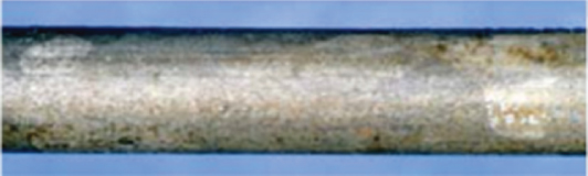
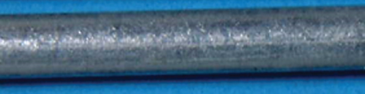
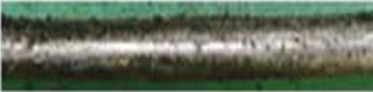
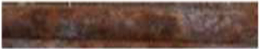
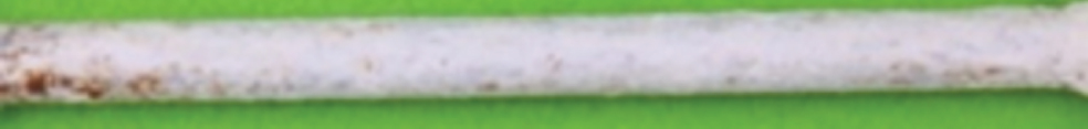
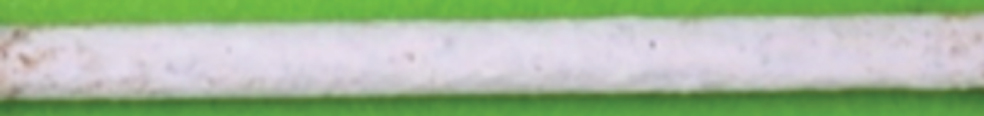
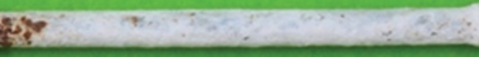
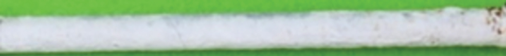
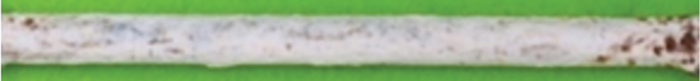
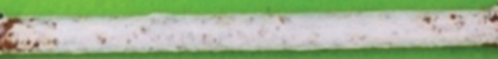
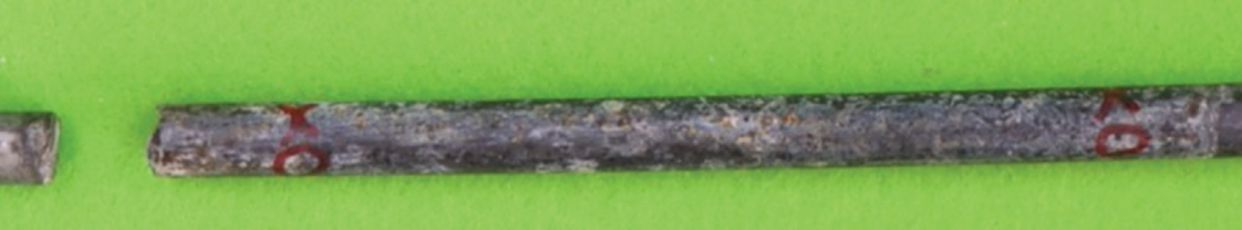
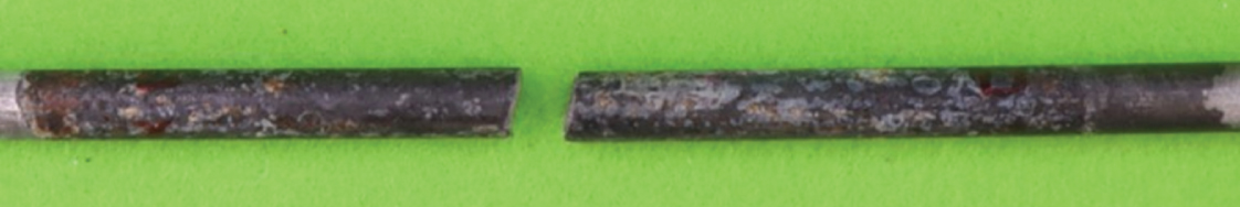
The specimens used in the test were high-strength galvanized steel wires used for cable-stayed bridges. The specimens were high-strength galvanized steel wires (hereinafter referred to as “wire”) with a diameter of 7 mm and a tensile strength of 1570 MPa, and a zinc coating of 331 g/m2 (equivalent to a plating thickness of about 50μm) was adhered to the surface of the wire. These specifications are identical to those mainly used for cable supported bridges with middle/long-span. The appearance of the wire before the corrosion acceleration test is shown in Fig. 1.
Fig. 1
High-strength galvanized steel wire.

The length of the specimens used in this study was 380 mm (chuck part for fatigue test 280 mm, corrosion part 100 mm), and a total of 8 specimens were used (6 for fatigue tests and 2 for tensile tests), and 13 new wires were used (11 for fatigue tests and 2 for tensile tests).
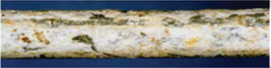
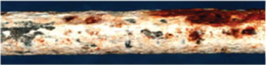
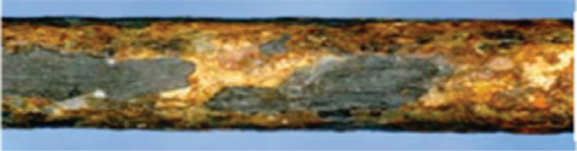
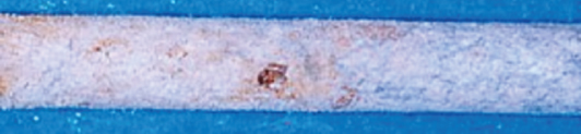
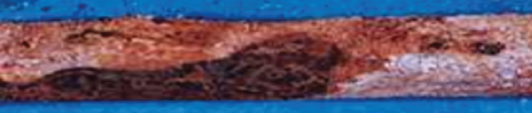
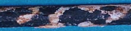
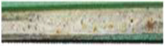
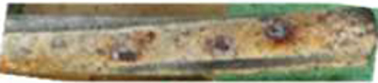
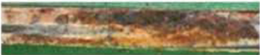
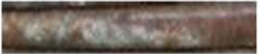
To manufacture corroded wires, a corrosion acceleration test was conducted. The corrosion acceleration test was carried out using the salt spray test method. The corrosion environment during the test was set to a constant temperature of 35C and humidity of 95%, and a 5% concentration of sodium chloride solution was sprayed [9]. Figure 2 shows the appearance of the test conditions. The test duration was 8,300 hours. Table 1 shows the results of the accelerated corrosion test. On the surface of the specimen after corrosion, white rust peculiar to the corrosion product of zinc and red rust peculiar to the corrosion product of the base iron were confirmed.
Fig. 2
Salt spray test.
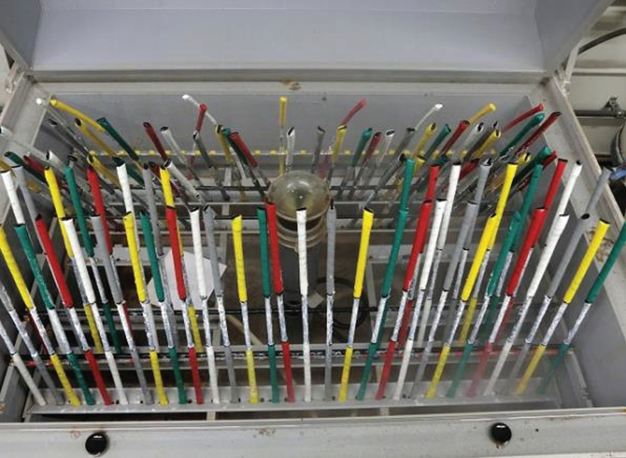
Table 1
Results of the accelerated corrosion test
| Specimen No. | Appearances |
| 1 | F 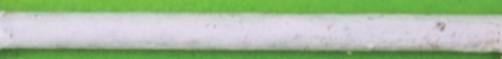 |
B 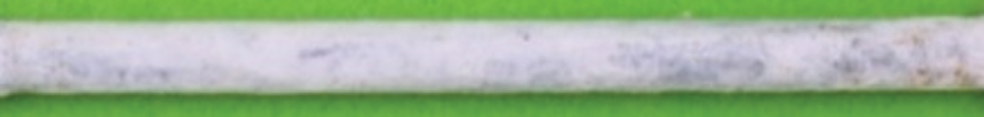 | |
| 2 | F  |
B 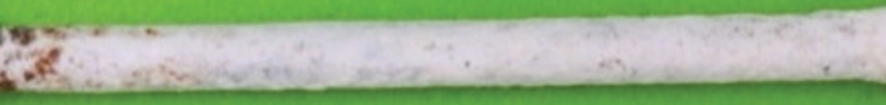 | |
| 3 | F 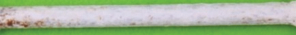 |
B  | |
| 4 | F 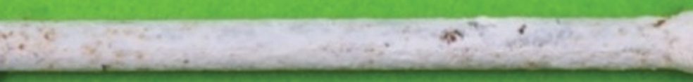 |
B 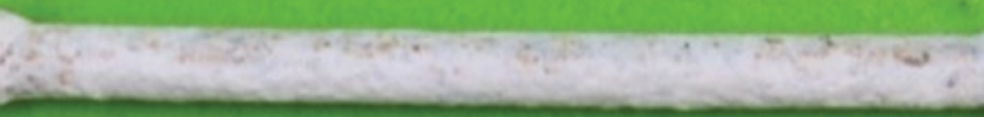 | |
| 5 | F  |
B 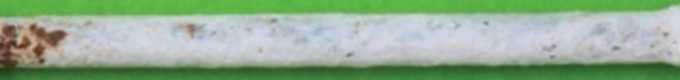 | |
| 6 | F  |
B  | |
| 7 | F  |
B  | |
| 8 | F  |
B 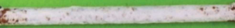 |
2.2Analysis methods
The object was captured, and the rust distribution ratio of each object was quantitatively grasped by digital image color analysis software from the captured image. The corrosion level of each object was classified based on the proportion of white rust specific to zinc and red rust specific to iron. After the corrosion acceleration test, the distribution and classification of the target rust color in the image of the appearance photograph of the corroded wire captured by a digital camera were displayed using the digital image color analysis system Feelimage Analyzer (Manufactured by Viva Computer, Inc.). The digital single-lens reflex camera (manufactured by Canon Inc., EOS Kiss X10) and the standard light source D65 [10] (Manufactured by Luci Co., Ltd.) specified by the International Commission on Illumination (CIE) were used for the shooting method, and it was installed as shown in Fig. 3.
Fig. 3
Shooting method.
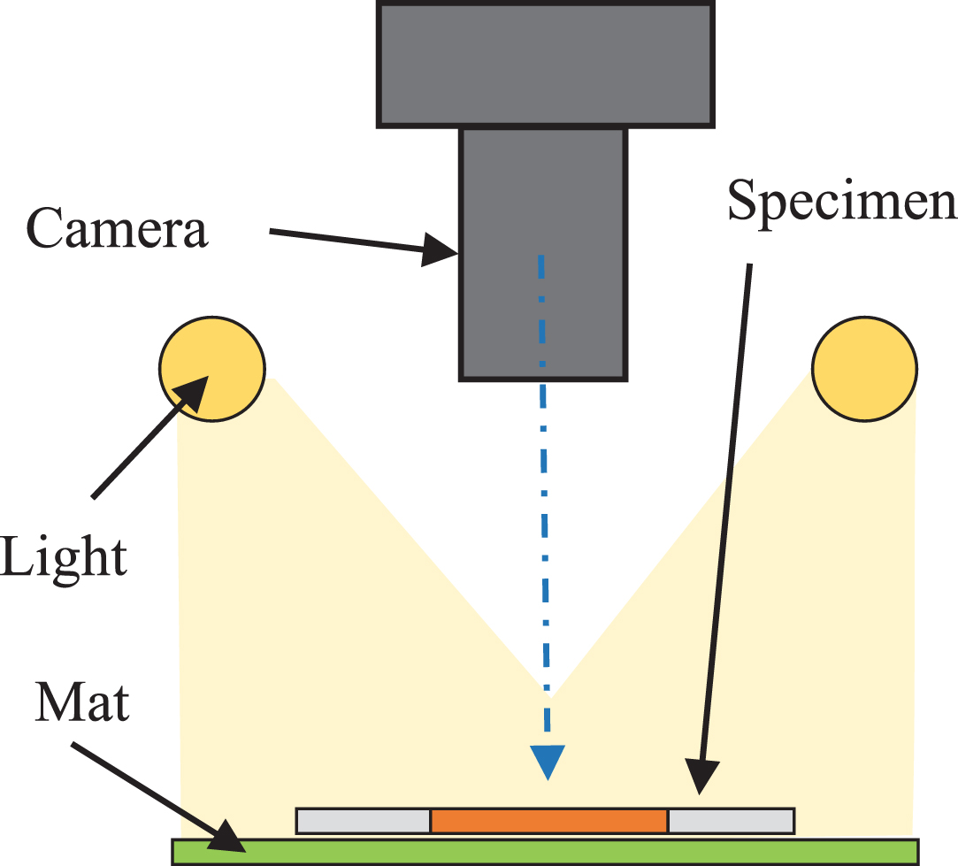
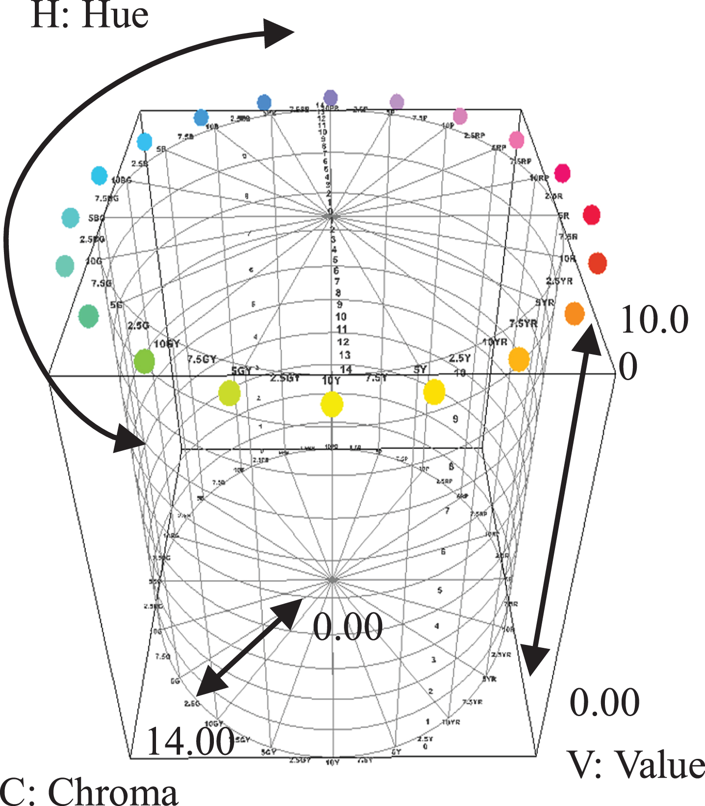
The camera shooting conditions were set to a shutter speed of 1/100 second, F-value of 22, and ISO sensitivity of 100, and each object was captured under the same conditions. In this analysis system, all pixels in the image are represented in a quantitative color system known as the Munsell color system, consisting of three dimensions: Munsell hue (H), Munsell value (V), and Munsell chroma (C) (as shown in Figure X). The analysis method involves setting a range of color hues, values, and chromas in the image and quantitatively classifying the amount of rust color present to categorize it.
Munsell hue (H) represents the difference in color tone. The system uses the five basic hues of red, yellow, green, blue, and purple (represented by R, Y, G, B, and P respectively), as well as the intermediate hues of yellow-red (YR), yellow-green (GY), blue-green (BG), blue-purple (PB), and red-purple (RP), resulting in a total of ten hues. Each hue is further subdivided into 100 levels ranging from 0.01 to 10.00 in the Munsell system.
Munsell value (V) represents the degree of brightness. Ideal white is represented by 10.00 and ideal black by 0.00, with brightness changing uniformly between them, and values are expressed in increments of 10. Since it is not possible to achieve ideal black and white, the darkest value is represented as 1, and the brightest value as 9.5.
Munsell chroma (C) indicates the degree of color saturation, with the distance from the achromatic color being represented. The higher the chroma, the more vivid the color, and the lower the chroma, the more achromatic the color. Chroma is expressed on a scale of 0.00 to 14.00, with a chroma of 0 indicating an achromatic color.
2.2.1Classification of background area and specimen area
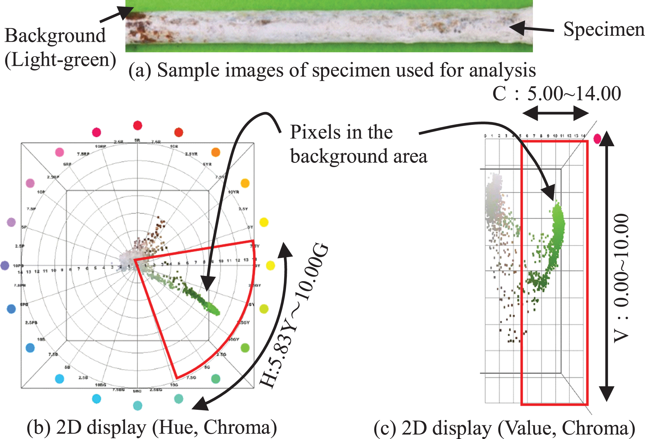
Firstly, the rust color observed on the test object was classified into two types: white rust, which is specific to zinc plating on wire surfaces, and red rust, which is specific to ground iron. When capturing images of the test object, a yellow-green background was set up in contrast to the above-mentioned rust color, making it easy to classify the rust color and background color. An example of analysis using a digital image color analysis system is shown in Fig. 4.
Fig. 4
Mansell color system.
The analysis procedure is explained using an image of a corroded wire (surface of specimen) that was captured. When the image to be analyzed is inserted into the system, it is displayed as a group of pixels in three dimensions on the Mansell scale. First, based on the two-dimensional representation of hue H and chroma C, as well as the two-dimensional representation of lightness V and chroma C, a color area such as that shown in the background color was subjectively selected, which was then designated as the background area. The color range of the background area was determined to be hue H: 5.83Y-10.00 G, lightness V: 0.00-10.00, chroma C: 5.00–14.00 (Fig. 5).
Fig. 5
Example of analysis using a digital image color analysis.
2.2.2Classification of white rust and red rust area
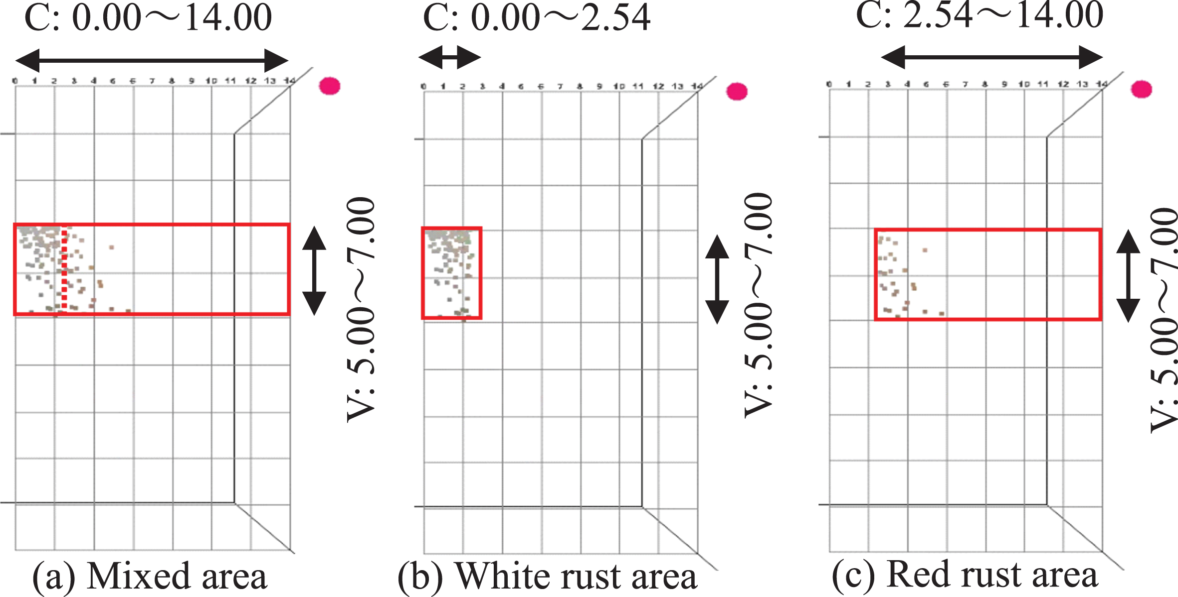
Next, subjectively classify the white rust and red rust areas by excluding the background area. As shown in Fig. 6, the white rust area is represented by the two-dimensional display of color phase H and color saturation C, where colors that are thought to be white rust are displayed throughout the color phase, so the white rust area was selected by choosing color phase H: 5.00 R to 5.00 R. Additionally, in the two-dimensional display of brightness V and color saturation C, brightness V: 7.00 to 10.00 and color saturation C: 0.00 to 5.00 were selected. As shown in Fig. 7, the red rust area was determined by the two-dimensional display of color phase H and color saturation C, where the color of red rust contrasts with the background color, and thus color phase H: 10.00 G to 5.83Y was selected. Additionally, in the two-dimensional display of brightness V and color saturation C, brightness V: 0.00 to 5.00 and color saturation C: 0.00 to 14.00 were selected. However, with the above area settings, a mixed area of white rust and red rust occurs, as shown in Fig. 8. Therefore, even within this area, white rust and red rust areas were subjectively classified. In the mixed area of white rust and red rust, the color of white rust and red rust changes depending on the degree of color saturation C. Thus, the white rust area was selected with brightness V: 5.00 to 7.00 and color saturation C: 0.00 to 2.54, and the red rust area was selected with brightness V: 5.00 to 7.00 and color saturation C: 2.54 to 14.00.
Fig. 6
White rust area setting.
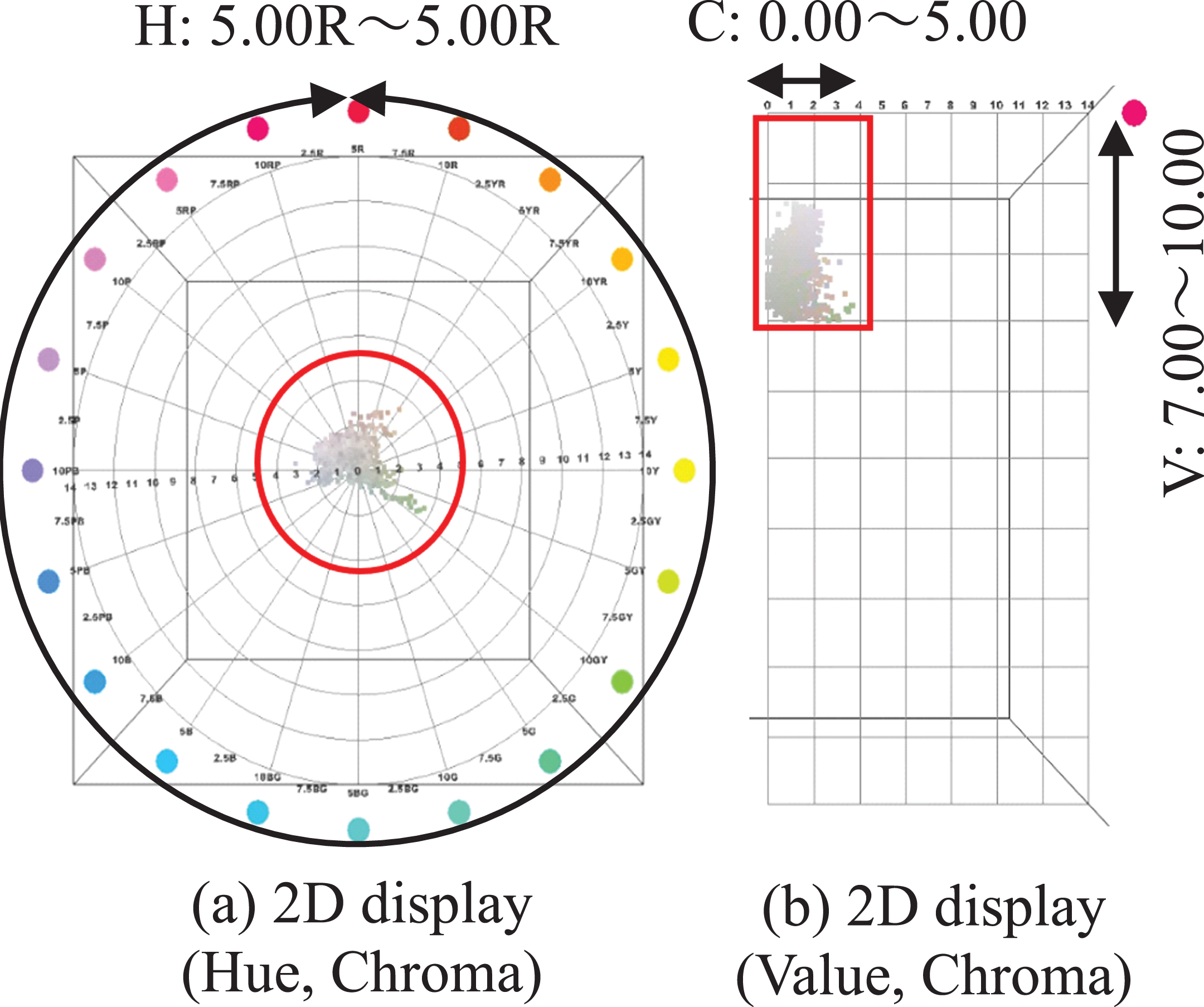
Fig. 7
Red rust area setting.
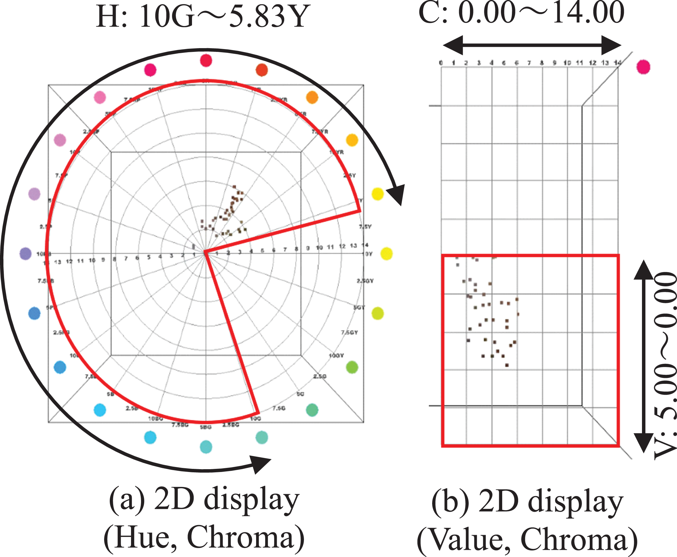
Fig. 8
Setting of mixed white/red rust area.
The color phase H was selected as in the above white rust and red rust area settings. Table 2 shows the color range setting values of color phase H, brightness V, and color saturation C in the background, white rust, red rust, and mixed areas. Table 3 shows corrosion classification schemes per [12], and [13].
Table 2
Setting range of hue H, Value V, and Chroma C
| Color area | H(Hue) | V(Value) | C(Chroma) |
| Background area | 5.83Y 10.00G | 0.00 10.00 | 5.00 14.00 |
| White rust area | 5.00R 5.00R | 7.00 10.00 | 0.00 5.00 |
| Red rust area | 10.00G 5.83Y | 0.00 5.00 | 0.00 14.00 |
| Mixed area (white rust) | 5.00R 5.00R | 5.00 7.00 | 0.00 2.54 |
| Mixed area (red rust) | 10.00G 5.83Y | 5.00 7.00 | 2.54 14.00 |
2.3Corrosion level setting
Inspections of actual stay and suspension cable bridge wires have revealed that deterioration starts with the depletion of the zinc coating, followed by mechanisms that involve surface corrosion and the formation of localized pits and transverse cracks. Based on field observations, wire corrosion has been categorized visually in four stages, as per [11]:
1 Stage 1— spots of zinc oxidation on the wires.
2 Stage 2— zinc oxidation on the entire wire surface.
3 Stage 3— spots of brown rust covering up to 30% of the surface of a 75–150 mm length of wire.
4 Stage 4— brown rust covering more than 30% of the surface of a 75–150 mm length of wire.
On the other hand, in accordance with the categorization proposed in [12], four corrosion levels can be distinguished:
1 Initial Stage — nearly initial condition of galvanized steel wire with almost no corrosion.
2 Level 1— wire covered by zinc-specific white rust and dots in places with iron-specific red rust.
3 Level 2— wire covered by white rust and locally red rust spread.
4 Level 3— corrosion in wire further progressed and red rust generation area increased.
Furthermore, a corrosion evaluation criterion, based on the rust color and its associated rust composition obtained from the appearance of the suspension bridge’s main cable, which has been in service for over 50 years, was proposed in [13]. In this context, the corrosion level has been subdivided into six stages:
1 Initial stage— At this stage, the galvanized steel wire is almost free from corrosion, and in its nearly initial condition. However, a black residue was observed on the surface of the wire, primarily on the center strand. Analysis of this residue revealed the presence of hydrocarbons, confirming it to be an oil-based component.
2 Level 1- This stage is characterized by the presence of zinc-specific white rust, accompanied by iron-specific red rust dots in some areas. Zinc carbonate, which is highly effective in preventing corrosion, was predominantly identified on the white rust.
3 Level 2- In this stage, the surface is covered by white rust with locally spread red rust. In addition to the features of Level 1, α-FeOOH, a stable rust with low activity, was also identified.
4 Level 3- Corrosion has progressed further, and there is an increased area of red rust generation. Along with the characteristics of Level 2, Fe3O4, a stable rust with low activity, has also been identified.
5 Level 4- Corrosion has further advanced, and there is an increased area of red rust generation. Additionally, zinc oxide with low anticorrosive properties has been identified, along with the features of Level 3.
6 Level 5- In this stage, corrosion has significantly progressed, with a large area of red rust generation. In addition to the characteristics of Level 4, γ-FeOOH, an active rust, has been identified.
As can be seen in Table 3, which compares the three categorization schemes, the development of the corrosion phenomenon appears to be quite similar.
However, it is important to note that the above assessment is based on visual observation, which may be subjective. In this study, therefore, a corrosion evaluation criterion based on image analysis techniques was investigated, considering above assessment. Table 4 shows the corrosion levels established in this study.
Table 4
Corrosion level setting in this study
| Corrosion level | White rust (%) | Red rust (%) |
| 0 | 0 | 0 |
| 1 | 100∼97 | 0∼3 |
| 2 | 97∼70 | 3∼30 |
| 3 | 70∼40 | 30∼60 |
| 4 | 40∼ | 60∼ |
2.4Analysis results
Based on the results of the analysis of the rust color distribution rate of the specimens analyzed in the previous process, the corrosion level was classified based on the proportion of white rust rate and red rust rate. The evaluation results of the rust color distribution rate and corrosion level are shown in Table 5. From these results, it became possible to quantitatively grasp the rust color distribution rate in each specimen. Furthermore, corrosion levels equivalent to corrosion levels 1 and 2 were confirmed, and the average rust color distribution rate and standard deviation at corrosion level 1 were white rust: 98.9±0.56%, red rust: 1.04±0.56%, and the average rust color distribution rate at corrosion level 2 was white rust: 95.3±0.67%, red rust: 4.65±0.67%.
Table 5
Evaluation results of the rust color distribution rate and corrosion level
| Specimen No. | Appearances | White rust (%) | Red rust (%) | Corrosion level | |
| 1 | F |
 | 99.7 | 0.27 | 1 |
| B |
 | ||||
| 2 | F |
 | 94.8 | 5.21 | 2 |
| B |
 | ||||
| 3 | F |
 | 98.2 | 1.78 | 1 |
| B |
 | ||||
| 4 | F |
 | 99.2 | 0.81 | 1 |
| B |
 | ||||
| 5 | F |
 | 95.0 | 4.98 | 2 |
| B |
 | ||||
| 6 | F |
 | 96.5 | 3.49 | 2 |
| B |
 | ||||
| 7 | F |
 | 98.7 | 1.31 | 1 |
| B |
 | ||||
| 8 | F |
 | 95.1 | 4.93 | 2 |
| B |
 |
3Corrosion surface shape
3.1Measurement method
In this section, the corrosion-generated products of the corroded test specimens were removed, and the quantitative measurements of the diameter, cross-sectional loss rate, and pit depth of each corrosion section of the specimens were obtained through the corrosion surface shape analysis and measurement method. As a measurement method, a general-purpose nylon brush and rust removal agent (abrasive) was used to remove the corrosion-generated products, taking care not to damage the plating or the base iron parts. At this time, the removal was carefully performed to ensure that there were no differences in the degree of removal for each test specimen.
Subsequently, the rust on the surface was removed after analyzing the rust distribution rate, and the surface characteristics of the corroded wire were measured using a handheld 3D scanner. The scanner used was the Artec Space Spider manufactured by Artec (California, USA, Fig. 9), which measures the object’s 3D surface features as if ironing the object. No markers need to be attached to the object as the handheld 3D scanner automatically captures the unique surface shape of the object and creates a 3D surface model by synthesizing it.
Fig. 9
Scan measurement.
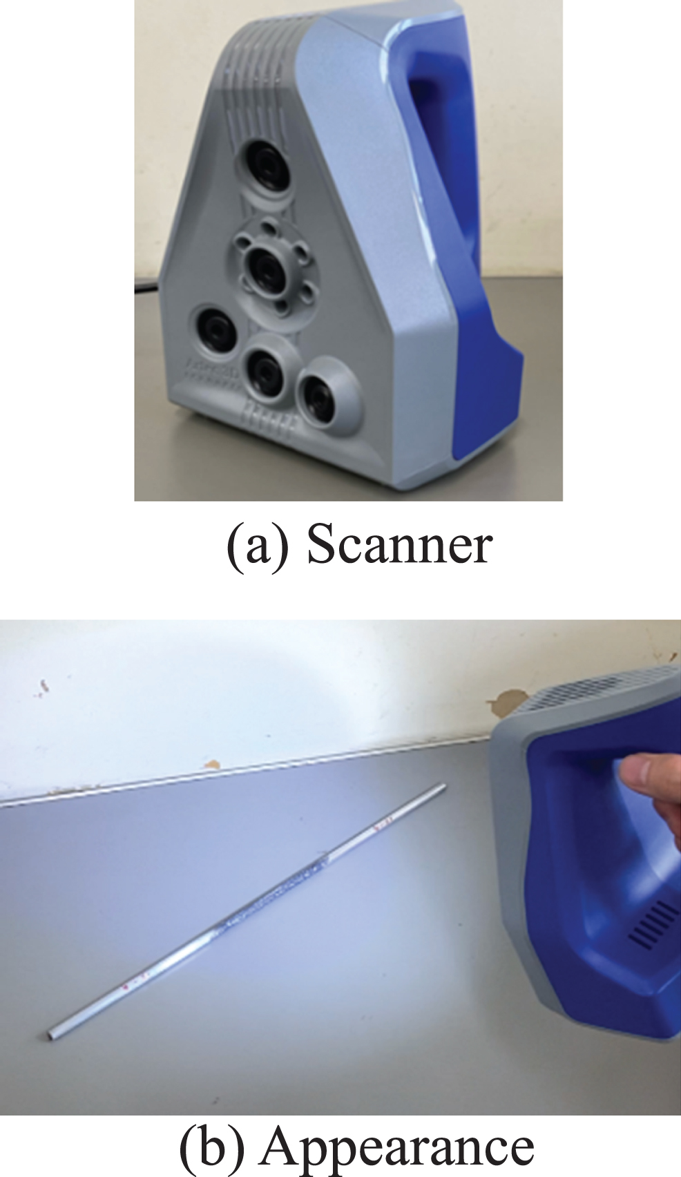
The object can be scanned while being held by hand, achieving a precision of 0.05 mm or less even in areas that are in shadow. The scanner captures images continuously while rotating at a speed of 15 images per second, and it can scan objects from those that fit in the palm of the hand to those that are several meters in size, measuring the entire object in a short time. Length measurement and cross-section creation are possible with the created model.
3.2Analysis method
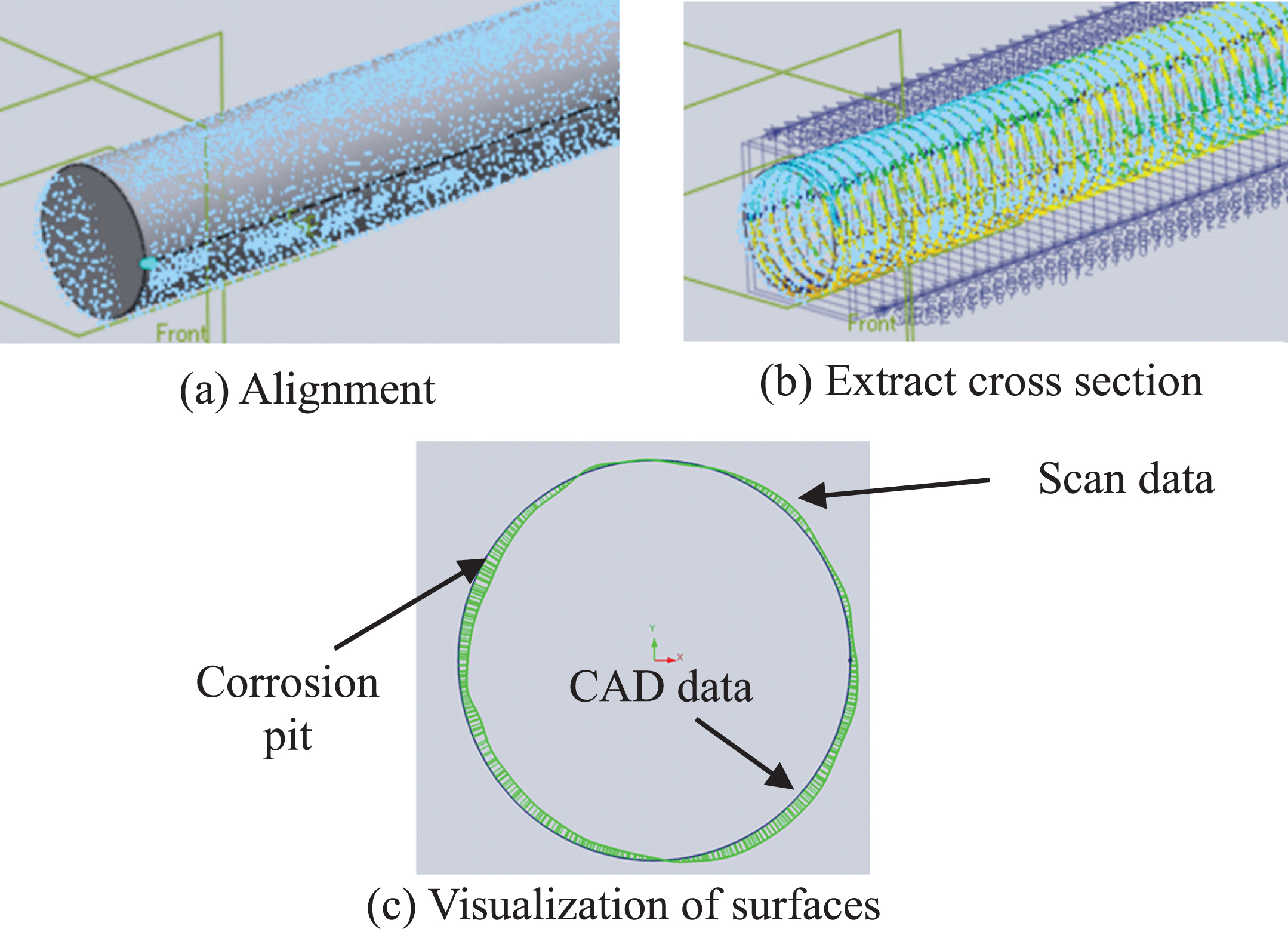
After scanning the test object, we analyzed the 3D corrosion wire surface shape (Scan data) using QA-Scan (Next Engine) to understand corrosion surface shape, area loss, corrosion depth, distribution, etc. By aligning Scan data and corrosion-free wire data generated by CAD (CAD data) on the same coaxial axis, we visualized the surface shape due to corrosion from the deviation between the data (Fig. 10). The cross-section of the test object’s corroded portion 101 times at 1 mm pitch along the length of the 100 mm length of the test object was analyzed. Next, using the corrosion wire surface measurement method proposed in [14], the area loss rate and the change in corrosion pit depth were calculated for each cross-section from the optimized Scan data. Furthermore, it should be noted that the wire used in this study has a zinc galvanizing thickness of approximately 50μm (0.05 mm). Therefore, the corrosion surface characteristics of corroded wires were adjusted by considering the subtraction of zinc galvanizing thickness.
Fig. 10
Surface profile measurement.
3.3Measurement results
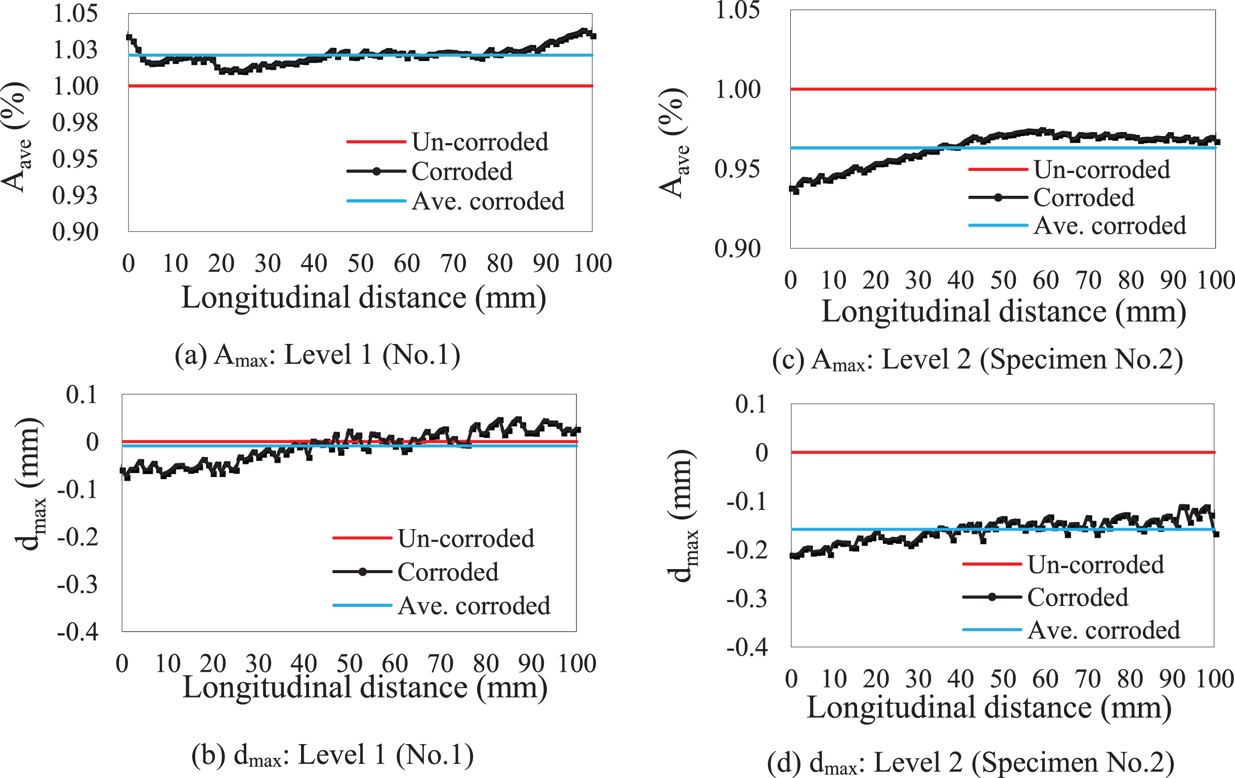
The analysis results are shown in Table 6. For corrosion level 1, the average cross-sectional loss rate Aave was – 0.4±1.1% (=– 1.5 0.7%), and the maximum corrosion pit depth dmax was 0.119±0.034% mm (= 0.085 0.153 mm). On the other hand, for corrosion level 2, the average cross-sectional loss rate Aave was 1.3±1.8% (=– 0.5 3.1%), and the maximum corrosion pit depth dmax was 0.231±0.053% mm (= 0.178 0.284 mm).
Table 6
Analysis results
| Specimen No. | Corrosion level | Aave
(%) | Amax( %) | dave
(mm) | dmax
(mm) |
| 1 | 1 | –2.1 | –1.0 | 0.009 | 0.073 |
| 3 | 1 | 1.0 | 4.2 | 0.047 | 0.135 |
| 4 | 1 | –0.2 | 1.5 | 0.084 | 0.164 |
| 7 | 1 | –0.2 | 3.3 | 0.016 | 0.103 |
| Ave. | –0.4 | 2.0 | 0.039 | 0.119 | |
| S.D. | 1.1 | 2.0 | 0.030 | 0.034 | |
| 2 | 2 | 3.7 | 6.4 | 0.158 | 0.211 |
| 5 | 2 | –0.8 | 3.3 | 0.169 | 0.313 |
| 6 | 2 | 2.2 | 5.9 | 0.076 | 0.168 |
| 8 | 2 | 0.1 | 4.7 | 0.086 | 0.231 |
| Ave. | 1.3 | 5.1 | 0.122 | 0.231 | |
| S.D. | 1.8 | 1.2 | 0.042 | 0.053 |
Figure 11 shows representative analysis results for corrosion levels 1 and 2. The results for the maximum cross-sectional area loss rate Amax and the maximum corrosion pit depth dmax, respectively, are shown in the longitudinal distance. When comparing corrosion levels 1 and 2, it can be quantitatively determined that corrosion level 2 has an approximately 0.9% higher average surface loss rate and a maximum corrosion pit depth about 0.112 mm deeper than corrosion level 1, indicating more advanced corrosion. Furthermore, similar trends were observed in other specimens at corrosion levels 1 and 2.
Fig. 11
Calculation method of section loss rate and corrosion pit depth.
4Fatigue strength
4.1Test method
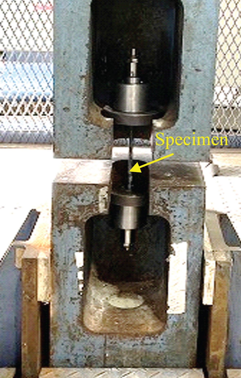
Finally, fatigue tests were carried out to investigate the influence of each corrosion level and corrosion roughness, as shown in sections 2 and 3, on the fatigue strength of each test specimen. After measuring the corrosion surface shapes, fatigue tests were conducted on both the corroded wire used in this study and the new wire to investigate the impact of corrosion on fatigue strength. Figure 12 shows the appearance of the test. The fatigue test was performed using an Electromagnetic resonance fatigue testing machine (Simadzu Co.), with a test specimen fixed to the testing machine. The minimum stress was set at 500 MPa, and the stress range was 600–700 MPa with a frequency of 10 Hz. In addition, fatigue tests were performed at three levels (700, 650, 600 MPa), with one test specimen per level, and the fatigue limit was performed at 2x10⁶ cycles, as proposed in [15].
Fig. 12
Fatigue test.
4.2Test results
The appearance of the fractured test specimens due to fatigue testing is shown in Table 7. In addition to the relationship between the stress range and the number of cycles leading to fracture (S-N curve), the relationship between rust color distribution rate and corrosion surface characteristics is summarized in Table 8.
Table 7
Appearance of specimen fracture in fatigue test
| No. | Appearances | Fracture position |
| 1 |
 | Corroded part |
| 2 |
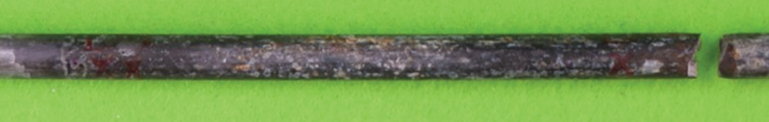 | Corroded part |
| 3 |
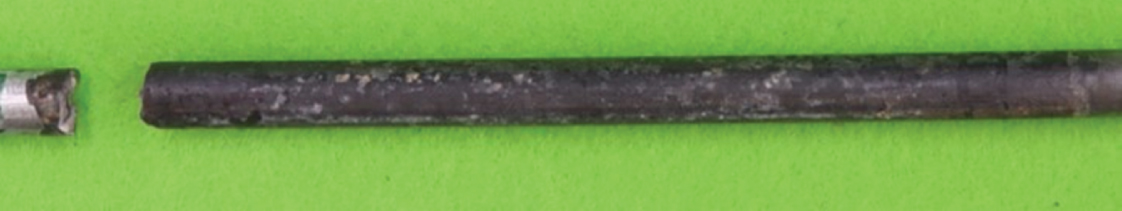 | Corroded part |
| 4 |
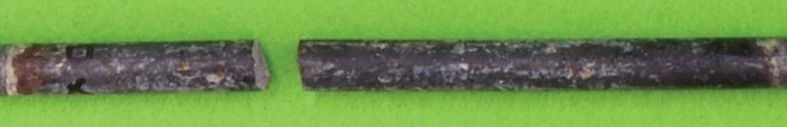 | Corroded part |
| 5 |
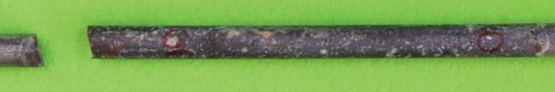 | Corroded part |
| 6 |
 | Corroded part |
Table 8
Relationship between rust color distribution, corrosion surface features, and fatigue strength
| Specimen | White rust | Red rust | Corrosion | Aave | Amax | dave | dmax | S | N |
| No. | (%) | (%) | level | (%) | (%) | (mm) | (mm) | (MPa) | (Cycles) |
| 1(new) | 0 | 0 | 0 | 0 | 0 | 0 | 0 | 700 | 9900 |
| 2(new) | 0 | 0 | 0 | 0 | 0 | 0 | 0 | 650 | 112000 |
| 3(new) | 0 | 0 | 0 | 0 | 0 | 0 | 0 | 650 | 94000 |
| 4(new) | 0 | 0 | 0 | 0 | 0 | 0 | 0 | 650 | 90000 |
| 5(new) | 0 | 0 | 0 | 0 | 0 | 0 | 0 | 650 | 75282 |
| 6(new) | 0 | 0 | 0 | 0 | 0 | 0 | 0 | 650 | 75000 |
| 7(new) | 0 | 0 | 0 | 0 | 0 | 0 | 0 | 600 | 924000 |
| 8(new) | 0 | 0 | 0 | 0 | 0 | 0 | 0 | 600 | 869000 |
| 9(new) | 0 | 0 | 0 | 0 | 0 | 0 | 0 | 600 | 472000 |
| 10(new) | 0 | 0 | 0 | 0 | 0 | 0 | 0 | 600 | 102000 |
| 11(new) | 0 | 0 | 0 | 0 | 0 | 0 | 0 | 600 | 65000 |
| No.1 | 99.7 | 0.27 | 1 | –2.1 | –1.0 | 0.009 | 0.073 | 700 | 313000 |
| No.4 | 99.2 | 0.81 | 1 | –0.2 | 1.5 | 0.084 | 0.164 | 650 | 153000 |
| No.3 | 98.2 | 1.78 | 1 | 1.0 | 4.2 | 0.047 | 0.135 | 650 | 142000 |
| No.2 | 94.8 | 5.21 | 2 | 3.7 | 6.4 | 0.158 | 0.211 | 700 | 69000 |
| No.6 | 96.5 | 3.49 | 2 | 2.2 | 5.9 | 0.076 | 0.168 | 650 | 608000 |
| No.5 | 95.0 | 4.98 | 2 | –0.8 | 3.3 | 0.169 | 0.313 | 650 | 521000 |
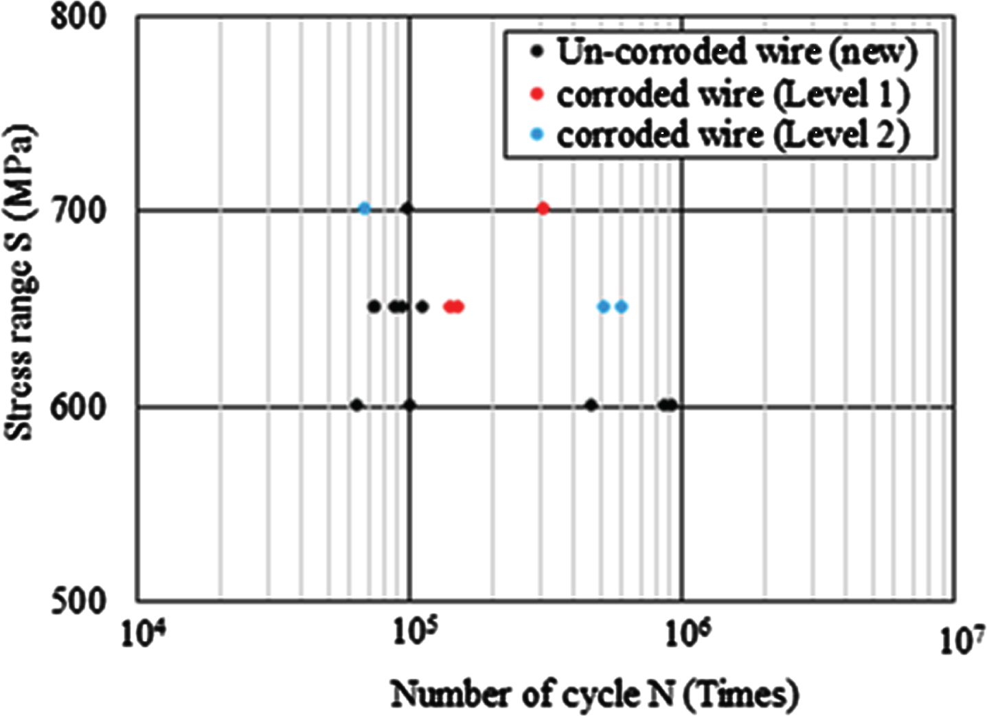
The S-N relationship of the new wire and corroded wires were shown in Fig. 13, from which it is evident that the fatigue strength of corroded wires exceeds that of new wires. This may be attributed to the inadequate consideration of variations caused by the small number of specimens tested, but it is also possible that corrosion did not progress to the extent of affecting wires made of steel with sufficient strength.
Fig. 13
S-N curve of new and corroded wire.
As part of the above-mentioned cause investigation, tensile tests were performed on the corroded wire and the new wire at corrosion levels 1 and 2, with one test specimen per level. The results of the tensile test are shown in Table 9. This indicates that all specimens exhibited a tensile strength of approximately 1570 MPa, and it is believed that the corrosion levels (1 and 2) set in this study may not sufficiently affect the fatigue strength.
Table 9
Tensile strength
| Corrosion level | Tension (MPa) |
| 0 | 1567 |
| 1 | 1567 |
| 2 | 1588 |
5Conclusions
This study examined the potential correlation between the “rust color distribution ratio,” “corrosion surface shape,” and “fatigue strength” of high-strength galvanized steel wires used in suspension bridge cables. The obtained results are summarized below.
• By introducing a digital image color analysis system in this study, the white rust unique to zinc and the red rust unique to iron from corroded wires and quantitatively grasp the rust color distribution rate were able to classify. Furthermore, by setting corrosion levels based on rust color distribution ratio, it has become possible to quantitatively categorize the levels.
• Additionally, from the quantitatively categorized corrosion levels, it has become possible to comprehend the relationship visually and quantitatively between cross-sectional loss rate and corrosion depth tendency, based on the increase or decrease in the rust rate.
• In the specimens obtained from the corrosion levels set in this study, fatigue strength showed results that were equivalent to or higher than those of new wires. The tensile strength also showed similar results. Therefore, it is considered that the corrosion levels (1 and 2) set in this study may not have a significant impact on fatigue strength. However, it should be noted that this may be due to insufficient consideration of variations resulting from the small number of specimens or the possibility that corrosion did not progress sufficiently to affect fatigue strength.
As a future research direction, it is imperative to augment the corrosion evaluation criteria of corroded galvanized steel wires by expanding the number of test specimens and to identify the criteria for strength degradation that occurs at corrosion level 1.
Moreover, although this study restricted its focus to corrosion levels 1 and 2, accruing more data by advancing the degree of corrosion in the test specimens can pave the way to establish precise indicators that account for the correlation of “rust color distribution rate,” “corrosion surface shape,” and “fatigue strength”.
Acknowledgements
In this study, the authors would like to acknowledge the support of the JSPS KAKENHI (Grant No. JP20K14810) and Tokyo Rope MFG. Co., Ltd. In addition, the authors would like to acknowledge the anonymous reviewers for their constructive comments and suggestions.
References
[1] | Stahl FL , Gagnon CP . Cable Corrosion, ASCE Press, (1996) . |
[2] | Betti R , Yanev B . Conditions of Suspension Bridge Cables, The New York City Case Study, Transportation Research Board Record (1999) ; 105–12. |
[3] | Mahmoud KM . Fracture strength for a high strength steel bridge cable wire with a surface crack, Theoretical and Applied Fracture Mechanics (2007) ; 48. |
[4] | Kameyama S , Hiramatsu T . Reinforcement work and long-term monitoring of steel suspension bridges due to partial breakage of main cables, 18th Civil Engineering Construction Management Technology Papers (2013) ; 111–4. |
[5] | Colford BR . Forth Road Bridge – maintenance and remedial works, Proceedings of the Institution of Civil Engineers, Bridge Engineering (2008) ;161: :125–32. |
[6] | Mahmoud KM . NYSDOT Report C-07-11, New York State Department of Transportation (NYSDOT), BTC method for evaluation of remaining strength and service life of bridge cables, NYSDOT, cosponsored by FHWA and New York State Bridge Authority. (2011) . |
[7] | U.S. Federal Highway Administration. Primer for the inspection and strength evaluation of suspension bridge cables, FHWA, Washington, DC, FHWA Report No. FHWA-IF-11-045. (2012) . |
[8] | Nakamura S , Miyachi K . Ultimate Strength and Chain-Reaction Failure of Hangers in Tied-Arch Bridges, Structural Engineering International. (2020) ;31: :136–46. |
[9] | JIS Z 2371: Methods of salt spray testing, (2015) . |
[10] | ISO 11664-2. CIE standard illuminants. (2007) . |
[11] | NCHRP Report 534. Guidelines for Inspection and Strength Evaluation of Suspension Bridge Parallel Wire Cable. (2004) ;17–25. |
[12] | Nakamura S , Suzumura K . Experimental Study on Fatigue Strength of Corroded Bridge Wires, Journal of Bridge Engineering. ASCE. (2013) ;18: (3):200–9. |
[13] | Kinoshita K , Yano Y , Hatasa Y , Hasuike R , Miyachi K . Examination of corrosion evaluation criteria based on rust composition analysis in corrosion investigation of actual suspension bridge main cables, Journal of Structural Engineering. (2020) ;66A: :431–42. |
[14] | MiyachiK, ChryssanthopoulosM, NakamuraS. Experimental assess-ment of the fatigue strength of corroded bridge wires using non-contact mapping techniques, Corrosion Science. (2021) ;178: . Available from: DOI: 10.1016/j.corsci.2020.109047. |
[15] | Japanese Society of Steel Construction. Cable-staye Steel Bridge, Steel Structures Series (1990) ;5: :40–45. |


