A top-level model of case-based argumentation for explanation: Formalisation and experiments

1.Introduction

There is currently an explosion of interest in automated explanation of machine-learning applications [2,26,31]. Some explanation methods explain the entire learned model (global explanation) while other methods explain an output in a specific case (local explanation). Also, some methods assume access to the model (model-aware explanation) while other methods assume no such access (model-agnostic explanation). This paper presents a model-agnostic method for (locally) explaining outcomes of learned classification models and evaluates it experimentally with three data sets. Our model-agnostic approach is motivated by the fact that access to a learned model often is impossible (since the application is proprietary) or uninformative (since the learned model is not transparent). We will only assume access to the training data and the possibility to observe a learned model’s output given input data. There are several model-agnostic explanation methods, including example-based methods, which explain a decision for a case by comparing it to similar cases in the training set [35]. We take a similar approach, drawing on AI & law research on argumentation with cases, which models how lawyers draw analogies to past cases and discuss their relevant similarities and differences. A case-based approach is natural since the training data of machine-learning algorithms can be seen as collections of cases. The resulting explanation model does not explain how a learned model reached a decision (it cannot do so since it has no access to the learned model) but under which assumptions the decision can be justified in terms of an argumentation model. Our explanation model thus not only provides better understanding of the decision but also grounds to critique it.

Our explanation model is top-level in that it itself gives no reasons for why differences between cases matter or can be downplayed but can be extended with more refined accounts of similarities or differences between cases in which such reasons are given. The model is formally defined as an instance of Dung’s well-known theory of abstract argumentation frameworks [24]. The results of our experimental evaluation studies indicate that our model is to some extent feasible in practice, but further development and more experimental studies, especially with human users and with extensions of our top-level model, are needed to confirm its usefulness as an explanation model. While our approach is motivated by legal decision making, it also applies to other kinds of decision making, such as commercial decisions about loan applications or employee hiring, as long as the outcome is binary and the input conforms to this paper’s factor- or dimension format.

There is so far little work on argumentation for model-agnostic explanation of machine-learning algorithms but recent research suggests the feasibility of an argumentation approach. We are inspired by the work of Čyras et al. [20,21], also applied by [18,19]. They define cases as sets of binary features plus a binary outcome (in [20] also a case’s ‘stages’ are considered, but for present purposes these can be ignored). Then they explain the outcome of a ‘focus case’ in terms of a graph structure that essentially utilises an argument game for grounded semantics of abstract argumentation semantics [24,32]. We want to use the latter idea while overcoming some limitations of Čyras et al.’s approach. First, they do not consider the tendency of features to favour one side or another, while in many applications information on these tendencies will be available. Second, their features are binary, while many realistic applications will have multi-valued features. Finally, they leave the precise nature in which their graph structures explain an outcome somewhat implicit. We want to address all three limitations in terms of recent AI & law work on case-based reasoning. A more detailed comparison with [20] will be given in Section 8.

As suggested by [31], good explanations are selective, contrastive and social. That an explanation is selective means that only the most salient points relevant to an outcome are presented. That an explanation is contrastive means that it not just explains why the given outcome was reached but also why another outcome was not reached. Finally, that an explanation is social means that in the transfer of knowledge, assumptions about the user’s prior knowledge and views influence what constitutes a proper explanation. In Section 10 we will argue that our model satisfies these criteria in several respects.

This paper is organised as follows. We present preliminaries in Section 2 and outline our general approach and its underlying assumptions in Section 3. We then present a boolean-factor-based definition of case-based explanation dialogues in Section 4 and extend it to multi-valued factors or ‘dimensions’ in Section 5. In Section 6 we report on experiments with datasets to evaluate our approach and in Section 7 we briefly discuss how our top-level model can be extended with more refined accounts of similarities and differences between cases. We then discuss related research in Section 8 after which in Section 9 we discuss in a more general sense whether our method is an explanation method or something else. We conclude in Section 10. Sections 2–5 are an extended and somewhat revised version of [37] while Section 6 is adapted from [41].

2.Preliminaries

In this section we describe some preliminaries. After a brief overview of AI & law research on case-based reasoning, we briefly summarise the theory of abstract argumentation frameworks and outline the factor-based theory of precedential constraint. The dimension-based version of the latter theory will be discussed later in Section 5.

2.3.Factor-based precedential constraint

For describing factor-based models of precedential constraint we first recall some notions concerning factors and cases often used in AI & law (e.g. in [27,28,43]), although sometimes with some notational differences. Let o and o′ be two outcomes and Pro and Con two disjoint sets of atomic propositions favouring, respectively, outcome o and o′. The variable s (for ‘side’) ranges over {o,o′} and s‾ denotes o′ if s=o while it denotes o if s=o′. We say that a set F⊆Pro∪Con favours side s (or F is pro s) if s=o and F⊆Pro or s=o′ and F⊆Con. For any set F of factors the set Fs⊆F consists of all factors in F that favour side s. A fact situation is any subset of Pro∪Con. A case is then a triple (pro(c),con(c),outcome(c)) where Pro≠∅ and outcome(c)∈{o,o′} (where we call pro(c)∪con(c) the fact situation of c). Moreover, pro(c)⊆Pro if outcome(c)=o and pro(c)⊆Con if outcome(c)=o′. Likewise, con(c)⊆Con if outcome(c)=o and con(c)⊆Pro if outcome(c)=o′. Finally, a case base CB is a set of cases.

Note that given the way the tendency of factors towards a particular outcome is defined, we cannot model dependency relations between factors. For example, we cannot model that one factor is pro an outcome only if another factor is present. In AI & law research on case-based reasoning with factors or dimensions there is a general assumption that factors or dimensions are independent from each other but this assumption may not always be warranted. The assumption also means that our model may be less suitable for explaining non-linear decision-making models.

We next summarise Horty’s [27] factor-based ‘result’ model of precedential constraint (the differences with his ‘reason model’ are irrelevant for present purposes, and hence not discussed here).

Definition 1

Definition 1(Preference relation on fact situations [27]).

Let X and Y be two fact situations. Then X⩽sY iff Xs⊆Ys and Ys‾⊆Xs‾.

X<sY is defined as usual as X⩽sY and Y≰sX. This definition says that Y is at least as good for s as X iff Y contains at least all pro-s factors that X contains and Y contains no pro-s‾ factors that are not in X.

Definition 2

Definition 2(Precedential constraint with factors [27]).

Let CB be a case base and F a fact situation. Then, given CB, deciding F for s is forced iff there exists a case c=(X,Y,s) in CB such that X∪Y⩽sF.

Horty thus models a fortiori reasoning in that an outcome in a focus case is forced if a precedent with the same outcome exists such that all their differences make the focus case as least as strong for their outcome as the precedent.

Definition 3.

A case base CB is inconsistent if and only if it contains two cases c and c′ with respectively, fact situations X and Y and outcomes s and s‾ such that X⩽sY (In that case deciding Y for both s and s‾ is forced). And CB is consistent if and only if it is not inconsistent.

As our running example we use a small part of the US trade secrets domain of the HYPO and CATO systems. We assume the following six factors along with whether they favour the outcome ‘misuse of trade secrets’ (π for ‘plaintiff’) or ‘no misuse of trade secrets’ (δ for ‘defendant’): the defendant had obtained the secret by deceiving the plaintiff (π1) or by bribing an employee of the plaintiff (π2), the plaintiff had taken security measures to keep the secret (π3), the information is obtainable elsewhere (δ1), the product is reverse-engineerable (δ2) and the plaintiff had voluntarily disclosed the secret to outsiders (δ3). We assume the following precedents:

c1(π):deceivedπ1,measuresπ3,obtainable-elsewhereδ1,disclosedδ3c2(δ):bribedπ2,obtainable-elsewhereδ1,disclosedδ3

Clearly, deciding a fact situation F for π is forced iff it has at least the π-factors {π1,π3} and at most the δ-factors {δ1,δ3} (by precedent c1), since then we have {π1,π3}⊆Fπ and Fδ⊆{δ1,δ3}. Likewise, deciding a fact situation for δ is forced iff it has at least the δ-factors {δ1,δ3} and at most the π-factor {π2} (by precedent c2).

Consider next the following fact situation:

F1:bribedπ2,measuresπ3,reverse-engδ2,disclosedδ3

Comparing F1 with c1 we must check whether {π1,π3,δ1,δ3}⩽π{π2,π3,δ2,δ3}. This is not the case, for two reasons. We have {π1,π3}⊈F1π={π2,π3} and we have F1δ={δ2,δ3}⊈{δ1,δ3}. Next, comparing with precedent c2 we must check whether {π2,δ1,δ3}⩽δ{π2,π3,δ2,δ3}. This is also not the case for two reasons. We have {δ1,δ3}⊈F1δ={δ2,δ3} and we have F1π={π2,π3}⊈{π2}. So neither deciding F1 for π nor deciding F1 for δ is forced. Henceforth we will assume it was decided for π.

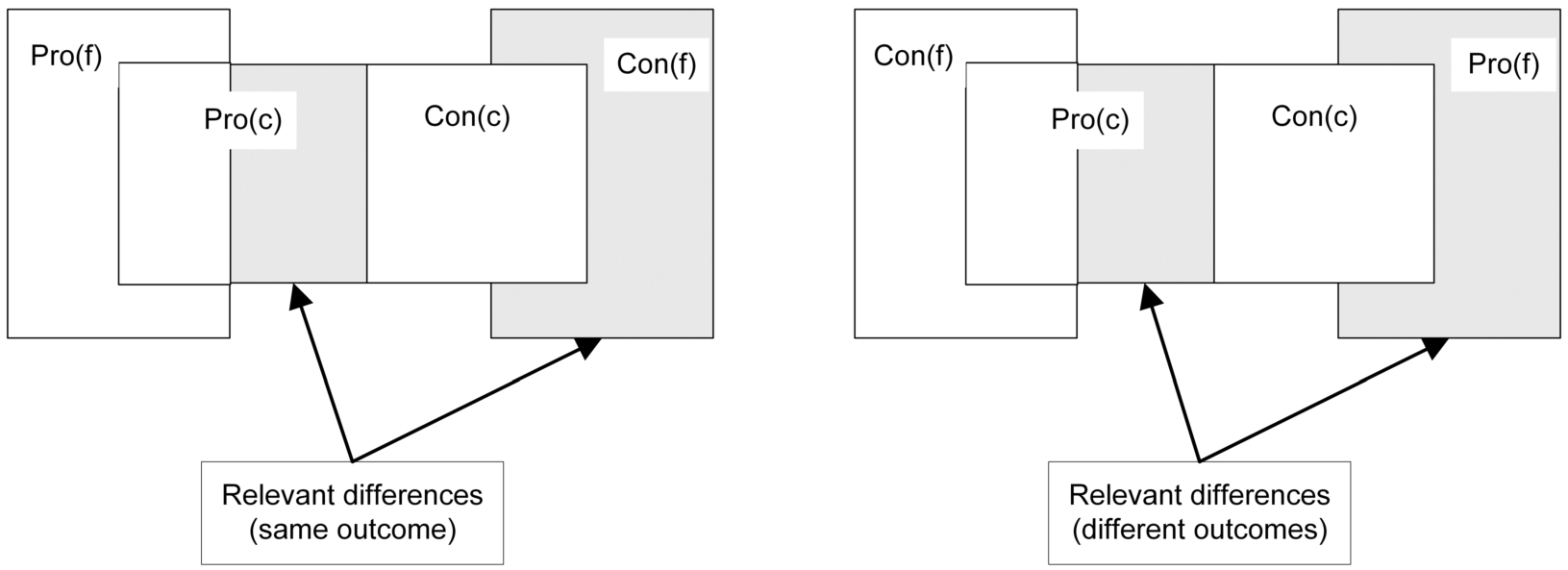
We finally recall some ideas and results of [38] and add a new result to them. In [38] a similarity relation is defined on a case base given a focus case and a correspondence is proven with Horty’s factor-based model of precedential constraint. The similarity relation is defined in terms of the relevant differences between a precedent and the focus case. These differences are the situations in which a precedent can be distinguished in a HYPO/CATO-style approach with factors [3,5], namely, when the new case lacks some factors pro its outcome that are in the precedent or has new factors con its outcome that are not in the precedent. To define the similarity relation, it is relevant whether the two cases have the same outcome or different outcomes.

If they have the same outcome, then a factor in the precedent that lacks in the focus case is only relevant if it is pro that outcome; otherwise its absence in the focus case only makes the focus case stronger than the precedent. Likewise, an additional factor in the focus case is only relevant if it is con the outcome. If the focus case and the precedent have opposite outcomes, then this becomes different. If the precedent has an additional factor that is pro the outcome in the precedent (so con the outcome in the focus case), then its missing in the focus case makes the focus case stronger than the other case, so it is a relevant difference. However, if the additional factor in the precedent is con the outcome in that case, then its missing in the focus case as (as a factor pro its outcome) makes the focus case weaker compared to the precedent. So this is not a relevant difference. On the other hand, if the focus case has an additional factor pro its outcome, then its addition to the precedent (as a factor con its outcome) might have changed its outcome, so this is a relevant difference between the cases. Finally, if the additional factor in the focus case is con its outcome, then adding it to the precedent (as a factor pro its outcome) strengthens the precedent, so this is not a relevant difference between the cases.

Definition 4

Definition 4(Differences between cases with factors [38]).

Let c and f be two cases. The set D(c,f) of differences between c and f is defined as follows.

• (1) If outcome(c)=outcome(f) then D(c,f)=pro(c)∖pro(f)∪con(f)∖con(c).

• (2) If outcome(c)≠outcome(f) then D(c,f)=pro(f)∖con(c)∪pro(c)∖con(f).

Figure 1 illustrates this definition.

Fig. 1.

Relevant differences D(c,f).

Consider again our running example and consider first any focus case f with outcome π and with a fact situation that has at least the π-factors {deceivedπ1,measuresπ3} and at most the δ-factors {obtainable-elsewhereδ1,disclosedδ3}. Then D(c,f)=∅. Likewise with any focus case f with outcome δ and with a fact situation that has at least the δ-factors {obtainable-elsewhereδ1,disclosedδ3} and at most the π-factor {bribedπ2}. Next, let f be a focus case with fact situation F1 and outcome π. We have

D(c1,f)={deceivedπ1,reverse-engδ2}D(c2,f)={measuresπ3,obtainable-elsewhereδ1}

The following result, which yields a simple syntactic criterion for determining whether a decision is forced, is proven in [38].

Proposition 1.

Let CB be a case base CB and F a fact situation. Then deciding F for s is forced given CB iff there exists a case c with outcome s in CB such that D(c,f)=∅, where f=(Fs,Fs‾,s).

We call a case citable given f iff it shares at least one factor pro its outcome with f and they have the same outcome [5]. Then clearly every case c such that D(c,f)=∅ is citable (recall that every case contains at least one factor pro its outcome).

As a new result, it can be proven that for any two cases with opposite outcomes that both have differences with the focus case, their sets of differences with the focus case are mutually incomparable (as with c1 and c2 in our running example). The proofs of all results in this paper are given in Appendix A.1.

Proposition 2.

Let CB be a case base, f a focus case and c and c′ two cases with opposite outcomes and with non-empty sets of differences with f. Then D(c,f)⊈D(c′,f) and D(c′,f)⊈D(c,f).

3.Approach and assumptions

We next sketch our general approach and its underlying assumptions. For a given classification model resulting from supervised learning we assume knowledge of the set of the model’s input features, i.e., factors or dimensions and a binary outcome, plus the ability to observe the output of the learned model for given input. We also assume knowledge about the tendency of the input factors or dimensions towards a specific outcome, plus access to the training set from which the classification model was learned (data plus label). We then want to generate an explanation for a specific input-output pair of the classification model (the focus case) in terms of similar cases in the training set. Later, in Section 7, we will briefly discuss a more general task where further domain specific information may be used to generate the explanation. It should be noted that there is one important difference between our approach and the ‘traditional’ case-based argumentation models described above in Section 2.1: in our approach the outcome of the case to be explained is given as input while in traditional approaches the outcome of the new case is an output of the model.

Since we have no access to the classification model, we do not know how the decision makers reasoned when deciding the cases in the training set. All we can do is generate the explanations in terms of a reasoning model that is arguably close to the domain, such as the above-described AI & law models of case-based argumentation. Accordingly, our aim is to investigate to what extent an explanation can be given in terms of these argumentation models.

There are a few important differences between our approach and more familiar model-agnostic local explanation techniques. Feature summary approaches, such as LIME [42], explain a prediction in terms of the contribution of features to the model’s decision. Our approach offers more context by explaining the decision relative to other instances (cases) in the data set. Providing this context can help answer contrastive questions, such as: ‘Why did c have outcome x rather than y?’.

A second important difference is that our model does not explain how the learned model reached its decision but how this decision can be justified in terms of another model. It may happen that the outcomes of a black-box classification model and the argumentation-based model of precedential constraint disagree for a given input in that the output given by the classification model is not forced by the argumentation model. Such a discrepancy does not imply that the argumentation model is wrong. It may also be that the learned classification model is wrong, since such models are rarely 100% accurate. If the two models disagree, it may be informative to show the user under which assumptions the outcome of the learned model is forced according to the argumentation model. The user can then decide whether to accept these assumptions. Accordingly, the information our explanations should provide is twofold: whether the focus case is forced, and if not, then what it takes to make it forced. Our explanation model can thus not only provide better understanding of the decision but also grounds to critique it. In Section 9 we will discuss these points in more detail.

4.Explanation with factors

We now present our top-level model for case-based explanation dialogues with factors, formalised as an application of the grounded argument game to a case-based abstract argumentation framework. The model is top-level in that it gives no reasons for why differences between cases matter or can be downplayed. In Section 7 we briefly discuss how our top-level model can be extended with more refined accounts of similarities and differences between cases in which such reasons can be given. The idea of our model is that the proponent starts a dialogue for the explanation of a given focus case f by citing a most similar precedent in the case base CB with the same outcome as the focus case. Then the opponent can cite counterexamples and can distinguish the initial precedent on its differences with the focus case. The proponent then replies to the distinguishing moves with arguments why these differences are irrelevant and to the counterexamples in a way explained below. An explanation then amounts to a winning strategy for the proponent in the argument game that defines explanation dialogues; such a winning strategy shows how all possible attacks of the opponent on the initial citation can be counterattacked.

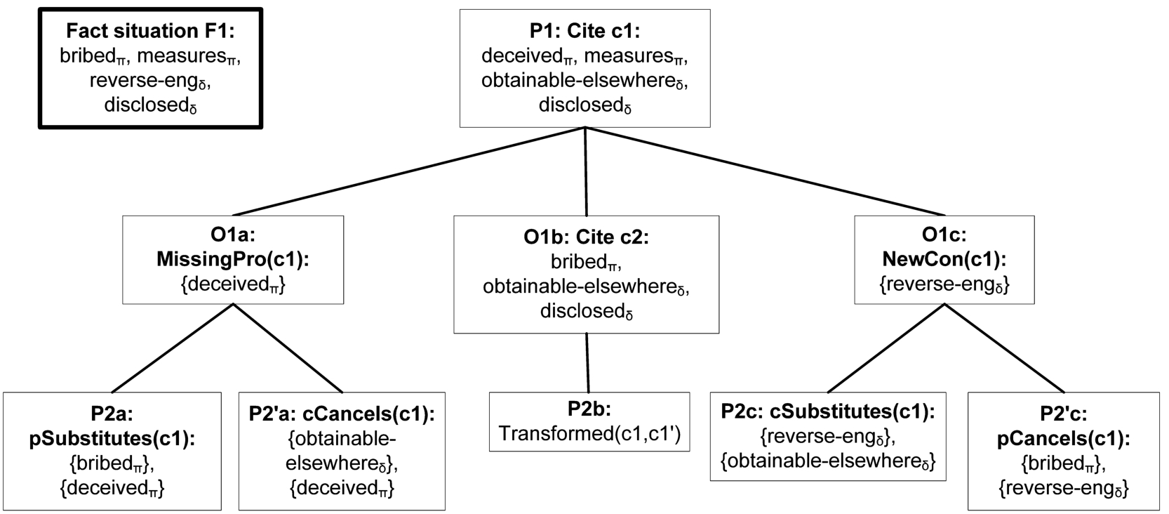
Definition 5 formalises these ideas in the form of a specification of a set of arguments plus an attack relation. We first informally introduce the definition. Figure 2 informally displays the two distinguishing moves and all ways to downplay them, while Fig. 3 shows how these moves can be used in our running example. Further example explanations (with both factors and dimensions) are given in Appendix A.2.

Fig. 2.

Distinguishing and downplaying distinctions.

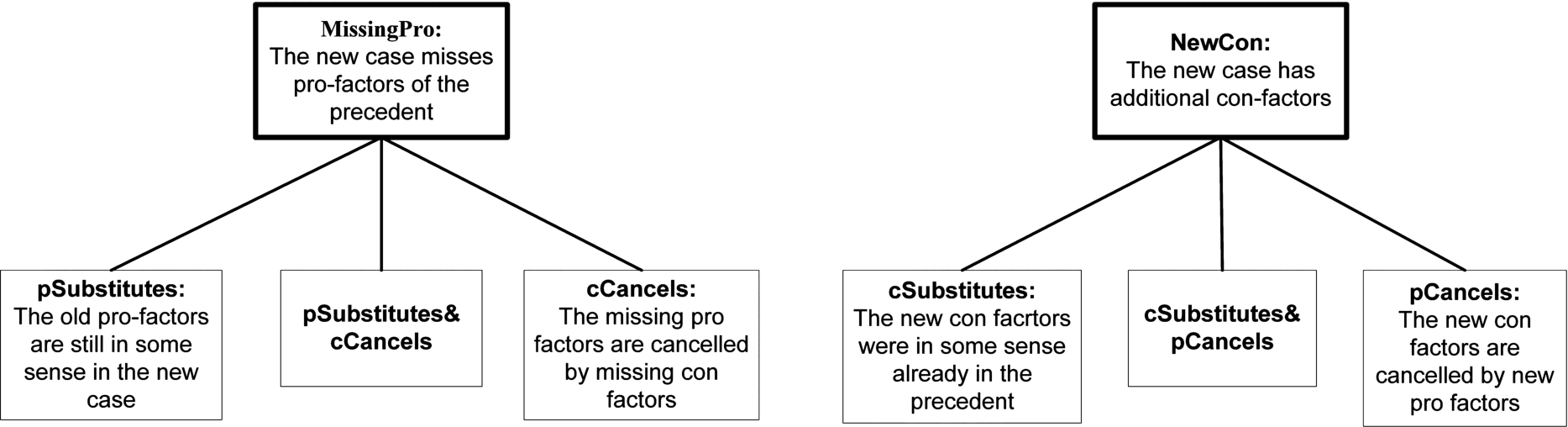
Fig. 3.

Example dialogue game tree.

The set A of arguments consists of a case base of precedents assumed to be citable given a focus case, plus a set M of arguments about precedents. Conflicts between precedents with opposite outcomes are resolved by using the similarity relation between precedents as a preference ordering between the precedents in A. The attack relations from members of M on members of A or M implicitly define the flow of the dialogue. The first two moves in M are meant as ‘distinguishing’ attacks on an initial citation of a precedent c. A MissingPro(c,x) move says that the focus case f lacks pro-s factors x of precedent c, while NewCon(c,x) says that the focus case f contains new con-s factors x that are not in precedent c. These moves correspond to the two ways of distinguishing a case in [3,5]. In our running example a citation of c1 can be a attacked by MissingPro(c1,{deceivedπ1}) and by NewCon(c1,{reverse-engδ2}).

The next six moves are meant as replies to such distinguishing moves. They are inspired by the ‘downplaying a distinction’ moves from [3] (although that work does not contain counterparts of our cSubstitutes and cCancels moves). The first two downplay a MissingPro move. First, a pSubstitutes(y,x,c) move says that the missing pro-s factors x are in a sense still in f, since they can be substituted with the new, similar pro-s factors y, so that the old preference in c for pro(c) over con(c) also holds for pro(f) over con(c). For example, in the US trade secrets domain both bribing an employee of the plaintiff and deceiving the plaintiff are questionable means to obtain the trade secret [3]. So in our running example the proponent can reply with pSubstitutes({bribedπ2},{deceivedπ1},c1). Second, a cCancels(y,x,c) reply says that the negative effect of the missing pro-s factors x in f is cancelled by the positive effect of the missing con-s factors y in f, so that the old preference in c for pro(c) over con(c) still holds for pro(f) over con(f). For example, the MissingPro(c1,{deceivedπ1}) attack can be counterattacked with cCancels(c1,{obtainable-elsewhereδ1},{deceivedπ1}).

There are also two ways to downplay a NewCon distinction. The cSubstitutes(y,x,c) move says that the new con-s factors y in f are in a sense already in the old case since they are similar to the old con-s factors x in c, so that the old preference in c for pro(c) over con(c) also holds for pro(c) over con(f). This move mirrors a p-substitutes move. In the US trade secrets domain, the two pro-δ factors that the information is obtainable elsewhere and that it was reverse-engineerable can both be seen as cases where the piece of trade information was known or elsewhere available [3]. So in our running example the proponent can reply with cSubstitutes({reverse-engδ2},{obtainable-elsewhereδ1},c1). Second, pCancels(y,x,c) says that the negative effect of the new con-s factors x in f is cancelled by the positive effect of the new pro-s factors y in f, so that the old preference in c for pro(c) over con(c) also holds for pro(f) over con(f). This moves mirrors a c-cancels move. For example, the NewCon(c1,{reverse-engδ2}) attack can be counterattacked with pCancels(c1,{bribedπ2},{reverse-engδ2}).

For now all these moves will simply be formalised as statements. Later, in Section 7, we briefly discuss how full-blown arguments can be constructed with premises supporting these statements. To this end, our formal definition of the set of arguments assumes an unspecified set sc of definitions of p- and c-substitution and p- and c-cancellation relations, as placeholders for explicit accounts of these notions. Note that all downplaying moves allow the factor sets used to downplay a distinction to be empty, as ways of saying that the differences between the precedent and the focus case do not matter.

A complication is how to handle that a MissingPro or NewCon argument can be attacked in different ways on different subsets of the missing pro-s or new con-s factors. For instance, two different missing pro factors may be p-substituted with two different new pro factors, or one subset of the missing pro factors can be p-substituted by new pro factors while another subset can be c-cancelled by missing con-s factors. The first situation can be accounted for in definitions in the set sc and will therefore be left implicit below. To deal with the second situation, the downplaying attacks will be formalised as combinations of an elementary p(c)-substitutes and/or c(p)-cancels move.

The last move is meant as a reply to a counterexample. For now its underlying idea can only be outlined. It is meant to say that an initial citation of a most similar case for the outcome of f can be transformed by the downplaying moves into a case with no relevant differences with f and which can therefore attack the counterexample. A more formal explanation can only be given after Definition 8.

Henceforth the arguments that attack a MissingPro or NewCon move are sometimes called downplaying moves.

The grounded argument game now directly applies. The idea (inspired by [20,21]) is to explain the focus case f by showing a winning strategy for the proponent in the grounded game, which guarantees that the citation of the focus case is in the grounded extension of the argumentation framework defined in Definition 5. Such a winning strategy shows how all possible attacks of the opponent on the initial citation can be counterattacked. In our approach, an explanation dialogue should start with a ‘best’ citable precedent c in CB with the same outcome s as the focus case f (best in that there is no c′∈CB with the same outcome as f and such that D(c′,f)⊂D(c,f)). Moreover, any Transformed(c,c′) move must have as c the dialogue’s initial move and as c′ a transformation of c into c′ during the dialogue according to Definition 8 below. Any strategy for the proponent that satisfies these constraints is an explanation for f. As will become clear below, these further constraints do not affect the existence of a winning strategy for at least one citation for the outcome of f.

Recall that a strategy for a player can be displayed as a tree of dialogues which only branches after that player’s moves and which contains all attackers of this move. A strategy for a player is then winning if all dialogues in the tree end with a move by that player; cf. [32].

One idea of our approach is that all moves in an explanation receive their meaning from (or are thus justified by) the formal theory of precedential constraint. To make this formal, we now specify the following operational semantics of the downplaying arguments in M as functions on the set of cases. The idea is that together these moves modify the root precedent of a strategy for the proponent into a case that makes f forced. Below Sy/x stands for the set obtained by replacing subset x of S with y.

In our running example we henceforth assume that O1a is attacked with P2a and O1c with P2c. Then c1 is transformed into a case c1′ as follows. First, pSubstitutes({bribedπ2},{deceivedπ1},c1) yields

Note that Lemma 3 justifies that a Transformed move attacks a citation of a counterexample, since it says that the moves in an explanation dialogue that downplay a distinction transform the initially cited case in the dialogue to a case with no relevant differences with the focus case. This means that the counterexample to the initial citation moved by the opponent loses its force, since it is not a counterexample to the transformed case. This is one illustration of the idea that an explanation dialogue identifies the assumptions that have to be accepted to justify a predicted outcome of the focus case.

One underlying reason that Proposition 4 holds is that a substituting or cancelling set can be empty, which is necessary to make the proponent win if the opposite outcome of the focus case is forced. Admittedly, such a justification of the outcome of the focus case is weak, but at least it informs a user that justifying the outcome of the focus case requires making the case base inconsistent. In all other cases where the outcome of f is not forced, the following proposition tells us that a winning strategy in fact transforms the initial precedent into a precedent that does control the focus case.

Together, our results formally capture the sense in which an explanation according to Definition 7 explains the focus case. If the focus case is forced, then any precedent with no relevant differences explains the focus case; if neither outcome is forced, then an explanation sequence of downplaying moves derived from the winning strategy explains what has to be accepted to make the focus case forced; and if the opposite outcome is forced, then explaining the outcome boils down to explaining that justifying the outcome of f requires making the case base inconsistent.

5.Explanation with dimensions

We next adapt the above-defined factor-based explanation model to cases with dimensions. We first outline some formal preliminaries.

6.Evaluation

In this section we report on experiments with three data sets to evaluate our approach. We in particular want to gain some initial insights into the circumstances under which our approach is feasible, and on which aspects it should be further developed or tested. We will evaluate the outcomes in terms of the nature of the generated explanations (size, comprehensibility, need for trivial explanations) and on how inconsistencies are dealt with. We first introduce the three data sets that were used for the experiments. After that, we discuss how the data instances were transformed into cases, making up the case bases. We then report on the experiments and evaluate the method based on the results. Recall that some example explanations for the three data sets are displayed in Appendix A.2.

7.Extending the top-level model

So far we have modelled explanation dialogues that only use information from the case base, that is, from the training set of the machine-learning application. However, depending on the nature of the application, more relevant information may be available, provided in advance by a knowledge engineer or during an explanation dialogue by a user. It is for this reason that our explanation model contains a thus far undefined set sc of definitions of why downplaying arguments can be played (hence the qualification ‘top-level’ model). We now briefly discuss how explicit definitions of this set can be given and how they can be used to provide the premises of downplaying arguments.

AI & law provides many insights here [10]. For example, the premises of pSubstitutes and cSubstitutes claims can be founded on a ‘factor hierarchy’ as defined for the CATO system [3,4]. We gave examples of this above. Furthermore, the pCancels and cCancels arguments can be said to express a preference for a set of pro factors over a set of con factors. In AI & law accounts have been developed of basing such preferences on underlying legal, moral or societal values, for example, by saying that deciding for a side on the basis of the presence of particular factors promotes or demotes particular legal or societal values. Arguments according to these accounts can provide the premises of arguments for the pCancels and cCancels claims. For example, move P2c′ from our running example could be based on a preference for promoting honesty over stimulating economic competition.

Applying these ideas requires that arguments have a richer internal structure, where the various claims become conclusions of inferences from sets of premises. One way to achieve this is to formalise relevant argument schemes in a suitable structured formal account of argumentation [29]. In [9,12,40] this approach was followed in the context of the ASPIC⁺ framework [33]. To give an idea of how the approach of these papers can be applied in the present context, we now semiformally sketch a few relevant argument schemes. The first is a scheme for cancelling new con factors with new pro factors: 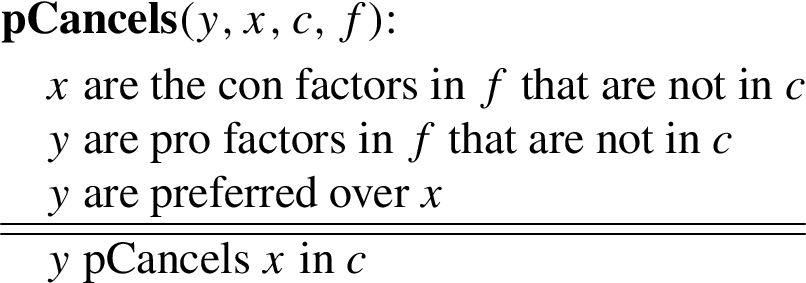The conclusion of this scheme can be defined as an undercutter of a similar scheme with conclusion ‘f has new con factors x that are not in c’. The pCancels scheme can be combined with a further argument scheme for arguing for preferences between factor sets on the basis of preferences between the sets of values promoted by these factor sets. The conclusion of this scheme in fact expresses that y pCancels x according to 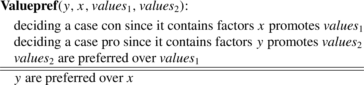sc (cf. Definition 5). We intend to further elaborate on these ideas in future research.

8.Related research

In this section we discuss related research on using case-based argumentation for explanation. A recent overview of AI & law models of explanation is [8]. An early suggestion to use example-based approaches for explaining machine-learning outcomes was [35]. Recently, the idea of ‘twin systems’ was proposed to explain artificial neural networks with case-based reasoning [30]. In this work a neural-network ‘black box’ model is mapped onto a more interpretable case-based reasoning system that works with the same data set as the neural net and that can be used to justify outputs of the neural net. The main focus in [30] is on methods for learning feature weights from neural networks for use in a k-nearest neighbor classifier. Similar methods could be useful for extensions of our current model with factor or dimension weights. Recent related work from AI & law is of Grabmair [25], who, adapting ideas of [17], predicts outcomes of legal cases in terms of factors and value judgements and explains these predictions with argumentation. While inspiring for our proposed research, his method relies on the use of an explicit argumentation model in the formulation of the classification problem, which he then uses for explaining the outcomes of the classifier. So his explanation method is, unlike our approach, not model agnostic. Finally, a recent empirical study suggests that a case-based style of explanation may lead to a lower degree of perceived justice than other styles [15]. We note that these experiments do not test for understandability of an explanation; it may be that the degree of perceived justice for case-based explanations is lower since they are more understandable than explanations of different kinds.

The closest to our approach and a main source of inspiration for us is Čyras et al.’s approach in [20,21]; it therefore deserves a detailed discussion and comparison. We here summarise the account of [20], where we will ignore their ‘stages’, which for present purposes are irrelevant. Cases in [20] are pairs of feature sets F and binary outcome o or o′. A case base (a set of cases) is assumed to be coherent in that two cases with the same sets of features cannot have opposite outcomes. On the basis of a case base an abstract argumentation framework is defined as follows. Arguments are cases. One case c=(F,o) attacks another c′=(F′,o′) iff F′⊂F (specificity) and there is no third case c″=(F″,o) such that F′⊂F″⊂F (conciseness). Conciseness says that only a least-specific case that is more specific than its target can attack the target. With this definition of attack, the resulting attack graph is acyclic, so in all four classical argumentation semantics an AF has the same unique extension [24]. Explanations are given in terms of ‘dispute trees’, which essentially are winning strategies in the argument game for grounded semantics. Although Čyras et al. do not use game-theoretic terminology, we will below still do so to facilitate the comparison with our approach. Games are about a focus case, which is not part of the case base and the outcome of which is to be explained. Games start with a default case (∅,δ), where δ∈{o,o′} is the default outcome. If the outcome of the focus case equals the default outcome, then the grounded game is played about the default case, otherwise it is played about any attacker of the default case. The idea is that the game identifies a dialogical proof of the default case if its outcome coincides with that of the focus case, or of at least one attacker of the default case if the outcome of the default case and the focus case differ.

Note that if F and F′ are not subsets of each other, then cases with these factor sets do not attack each other even though they have opposite outcomes. At first sight, this would seem to yield a problem. Consider δ=o and we have two cases c1=({f1},o) and c2=({f2},o′), of which c2 is the case to be explained. The game about the default case (assuming it has outcome o) would then end after c1 attacks the default case. Čyras et al. solve this problem by adding the focus case as a special argument to AF that attacks all arguments which contain features that are not in the focus case. Then the game in this example ends after c2 is moved to attack c1. The excess features of a strategy is the set of features of all cases in the strategy attacked by the focus case (here {f1}). Čyras et al. then define an explanation of the focus case as (in our terms) a pair consisting of a winning strategy plus its set of excess features, where the winning strategy is for the default case if it has the same outcome as the focus case and for an attacker of the default case otherwise.

Now because of the chosen attack relations (and since we ignore Čyras et al.’s stages) there will, if adding the focus case to CB leaves CB coherent, always be a winning strategy for the outcome of the focus case, while, moreover, the union of the sets of factors of the pro arguments in the proof is a subset of those of the focus case. The focus case itself does not necessarily appear in the proof; it will only if cases exist with the opposite outcome and features that are not in the focus case. The only kind of case where the outcome of the focus case does not have to be in the grounded extension is when there is a case in CB with the same features as the focus case but the opposite outcome.

While this approach is very interesting, it also has some limitations. First of all, the features are binary, while many realistic applications will have multi-valued features. Furthermore, the model does not represent the tendency of features (from now on ‘factors’) to support a particular outcome. When factors can be pro or con an outcome, then cases with factors not shared by the focus case can be informative, so that the design decision to have cases attacked by the focus case can result in loss of information relevant for explaining an outcome. Suppose, for example, that a focus case has outcome o with pro-o factor p1 and con-o factor c1 while a case in the case base also has outcome o and all factors of the focus case plus con-o factor c2. Then in our approach the outcome in the focus case can be explained by a fortiori reasoning from the second case. However, Čyras et al. generate a trivial dispute tree consisting just of the default case (if it has the same outcome as the focus case) or else of the default case followed by the focus case. The problem with this is that the case from the case base that justifies the decision in the focus case does not appear in the explanation.

Another limitation is that since Čyras et al. do not model the tendency of features, they are forced to have a broader notion of consistency (which they call ‘coherency’) for case bases, in which a case base is only inconsistent if it contains two cases with exactly the same features but opposite outcomes. This makes that situations where one case is even better for an outcome than another case but still has the opposite outcome, go unnoticed in their model, while in our approach they make the case base inconsistent. We regard this as an advantage of our approach, since many realistic applications will have case bases that are inconsistent in our sense and, as we argued above in Section 6.3, noting such inconsistencies may give meaningful information to a user.

We finally compare the explanations generated by Čyras et al. in our running example to the explanations generated by our method. If the default outcome is π then they generate the following winning strategy:

9.Explaining predictions of another classifier: Explaining, justifying or comparing?

In the previous section we discussed alternative example- and argumentation-based methods for explaining black-box classifiers. Yet a more general discussion of how to deal with black-box models is in order. As we noted at the end of Section 3, it may happen that the outcomes of a black-box classification model and the argumentation-based model of precedential constraint disagree for a given input in that the output given by the classification model is not forced according to the argumentation model. We proposed that in such cases it may be informative to show the user under which assumptions the outcome of the learned model is forced according to the argumentation model. This is captured in our operational semantics of the moves in an explanation dialogue, which for a focus case with non-forced outcomes shows how a best precedent is transformed through the dialogue into a case that forces the outcome of the focus case. Our explanation model can thus provide grounds to critique a learned model. Yet this also means that our explanation model does not simply explain how the classification model made its classification for the focus case. Instead of explaining how a black-box model comes to a prediction, our method explains how a different, more interpretable model can justify the prediction made. As a result, the explanation can fully deviate from the way the prediction model works.

At first sight, this would seem to make one of Rudin’s [45] criticisms apply to our method, namely, the criticism that our explanation system must as a separate classifier be worse than the prediction model, since otherwise the explanation system would make the prediction model redundant. Rudin’s worry is that given that the explanation system is worse, the system might distract the user from following correct predictions of the black-box. Yet this is not how our explanation system works; as Propositions 4 and 10 show, our explanation method is not designed to generate separate predictions that can be compared to those of the black-box classifier but to generate justified arguments for the black-box predictions, where the dialectical proofs of why these arguments are justified reveal the assumptions under which they are justified.

Because of her worries, Rudin proposes that at least for high-stake decisions, the aim should not be to explain black-box machine learning models but to design interpretable models instead. In fact, in [18,19] the model of Čyras et al. was not applied to explain a separate prediction model but to generate predictions itself, which were then claimed to be explainable since they were in argumentation-based form (see also the approach of [25]). For example, in [18] the model was applied to the Mushroom data set after an autoencoder neural network was first used to trim down the feature space. The argumentation classifier was then shown to perform better than a neural-network and a decision-tree classifier (though as noted above in Section 6.2.4, several 100% accurate classifiers for this data set are available). Although Rudin offers very valuable insights into the pros and cons of the various approaches, in our opinion the only way to know what is the right approach is by developing, applying and testing each of them. And in this paper we have developed and tested one way of modelling the explanation approach.

References

[1] | M.S. Acharya, A. Armaan and A.S. Antony, A comparison of regression models for prediction of graduate admissions, in: 2019 International Conference on Computational Intelligence in Data Science (ICCIDS), (2019) . doi:10.1109/iccids.2019.8862140. |
[2] | A. Addadi and M. Berrada, Peeking inside the black box: A survey on explainable artificial intelligence (XAI), IEEE Access ((2018) ). doi:10.1109/ACCESS.2018.2870052. |
[3] | V. Aleven, Using background knowledge in case-based legal reasoning: A computational model and an intelligent learning environment, Artificial Intelligence 150: ((2003) ), 183–237. doi:10.1016/S0004-3702(03)00105-X. |
[4] | V. Aleven and K.D. Ashley, Doing things with factors, in: Proceedings of the Fifth International Conference on Artificial Intelligence and Law, ACM Press, New York, (1995) , pp. 31–41. |
[5] | K.D. Ashley, Toward a computational theory of arguing with precedents: Accomodating multiple interpretations of cases, in: Proceedings of the Second International Conference on Artificial Intelligence and Law, ACM Press, New York, (1989) , pp. 39–102. |
[6] | K.D. Ashley, Modeling Legal Argument: Reasoning with Cases and Hypotheticals, MIT Press, Cambridge, MA, (1990) . |
[7] | K.D. Ashley, Artificial Intelligence and Legal Analytics. New Tools for Law Practice in the Digital Age, Cambridge University Press, Cambridge, (2017) . |
[8] | K. Atkinson, T.J.M. Bench-Capon and D. Bollegala, Explanation in AI and law: Past, present and future, Artificial Intelligence 289: ((2020) ), 103387. doi:10.1016/j.artint.2020.103387. |
[9] | K.D. Atkinson, T.J.M. Bench-Capon, H. Prakken and A.Z. Wyner, Argumentation schemes for reasoning about factors with dimensions, in: Legal Knowledge and Information Systems. JURIX 2013: The Twenty-Sixth Annual Conference, K.D. Ashley, ed., IOS Press, Amsterdam, (2013) , pp. 39–48. |
[10] | T.J.M. Bench-Capon, HYPO’s legacy: Introduction to the virtual special issue, Artificial Intelligence and Law 25: ((2017) ), 205–250. doi:10.1007/s10506-017-9201-1. |
[11] | T.J.M. Bench-Capon and K.D. Atkinson, Dimensions and values for legal CBR, in: Legal Knowledge and Information Systems. JURIX 2017: The Thirtieth Annual Conference, A.Z. Wyner and G. Casini, eds, IOS Press, Amsterdam, (2017) , pp. 27–32. |
[12] | T.J.M. Bench-Capon, H. Prakken, A.Z. Wyner and K. Atkinson, Argument schemes for reasoning with legal cases using values, in: Proceedings of the Fourteenth International Conference on Artificial Intelligence and Law, ACM Press, New York, (2013) , pp. 13–22. doi:10.1145/2514601.2514604. |
[13] | T.J.M. Bench-Capon and G. Sartor, A model of legal reasoning with cases incorporating theories and values, Artificial Intelligence 150: ((2003) ), 97–143. doi:10.1016/S0004-3702(03)00108-5. |
[14] | D.H. Berman and C.D. Hafner, Representing teleological structure in case-based legal reasoning: The missing link, in: Proceedings of the Fourth International Conference on Artificial Intelligence and Law, ACM Press, New York, (1993) , pp. 50–59. |
[15] | R. Binns, M. Van Kleek, M. Veale, U. Lyngs, J. Zhao and N. Shadbolt, ‘it’s reducing a human being to a percentage’; perceptions of justice in algorithmic systems, in: Proceedings of the 2018 CHI Conference on Human Factors in Computing Systems (CHI 2018), ACM Press, New York, (2018) , pp. 377:1–377:14. |
[16] | L.K. Branting, Data-centric and logic-based models for automated legal problem solving, Artificial Intelligence and Law 25: ((2017) ), 5–27. |
[17] | S. Brueninghaus and K.D. Ashley, Generating legal arguments and predictions from case texts, in: Proceedings of the Tenth International Conference on Artificial Intelligence and Law, ACM Press, New York, (2005) , pp. 65–74. |
[18] | O. Cocarascu, K. Čyras and F. Toni, Explanatory predictions with artificial neural networks and argumentation, in: Proceedings of the IJCAI/ECAI-2018 Workshop on Explainable Artificial Intelligence, (2018) , pp. 26–32. |
[19] | O. Cocarascu, A. Stylianou, K. Čyras and F. Toni, Data-empowered argumentation for dialectically explainable predictions, in: Proceedings of the 24th European Conference on Artificial Intelligence (ECAI 2020), (2020) , pp. 2449–2456. |
[20] | K. Čyras, D. Birch, Y. Guo, F. Toni, R. Dulay, S. Turvey, D. Greenberg and T. Hapuarachchi, Explanations by arbitrated argumentative dispute, Expert Systems With Applications 127: ((2019) ), 141–156. doi:10.1016/j.eswa.2019.03.012. |
[21] | K. Čyras, K. Satoh and F. Toni, Explanation for case-based reasoning via abstract argumentation, in: Computational Models of Argument, P. Baroni, T.F. Gordon, T. Scheffler and M. Stede, eds, Proceedings of COMMA 2016, IOS Press, Amsterdam, (2016) , pp. 243–254. |
[22] | K. Das and R.N. Behera, A survey on machine learning: Concept, algorithms and applications, International Journal of Innovative Research in Computer and Communication Engineering 5: (2) ((2017) ), 1301–1309. |
[23] | D. Dua and C. Graff, UCI Machine Learning Repository, (2019) , http://archive.ics.uci.edu/ml. |
[24] | P.M. Dung, On the acceptability of arguments and its fundamental role in nonmonotonic reasoning, logic programming, and n-person games, Artificial Intelligence 77: ((1995) ), 321–357. doi:10.1016/0004-3702(94)00041-X. |
[25] | M. Grabmair, Predicting trade secret case outcomes using argument schemes and learned quantitative value effect tradeoffs, in: Proceedings of the 16th International Conference on Artificial Intelligence and Law, ACM Press, New York, (2017) , pp. 89–98. |
[26] | R. Guidotti, A. Monreale, S. Ruggieri, F. Turini, F. Giannotti and D. Pedreschi, A survey of methods for explaining black box models, ACM Computing Surveys 51: (5) ((2019) ), 93:1–93:42. |
[27] | J. Horty, Rules and reasons in the theory of precedent, Legal Theory 17: ((2011) ), 1–33. doi:10.1017/S1352325211000036. |
[28] | J. Horty, Reasoning with dimensions and magnitudes, Artificial Intelligence and Law 27: ((2019) ), 309–345. doi:10.1007/s10506-019-09245-0. |
[29] | A.J. Hunter (ed.), Argument and Computation, 5: ((2014) ), Special issue with Tutorials on Structured Argumentation. |
[30] | E.M. Kenny and M.T. Keane, Twin-systems to explain artificial neural networks using case-based reasoning: Comparative tests of feature-weighting methods in ANN-CBR twins for XAI, in: Proceedings of the 28th International Joint Conference on Artificial Intelligence (IJCAI-19), (2019) , pp. 2708–2715. |
[31] | T. Miller, Explanation in artificial intelligence: Insights from the social sciences, Artificial Intelligence 267: ((2019) ), 1–38. doi:10.1016/j.artint.2018.07.007. |
[32] | S. Modgil and M. Caminada, Proof theories and algorithms for abstract argumentation frameworks, in: Argumentation in Artificial Intelligence, I. Rahwan and G.R. Simari, eds, Springer, Berlin, (2009) , pp. 105–129. doi:10.1007/978-0-387-98197-0_6. |
[33] | S. Modgil and H. Prakken, The ASPIC+ framework for structured argumentation: A tutorial, Argument and Computation 5: ((2014) ), 31–62. doi:10.1080/19462166.2013.869766. |
[34] | C. Molnar, Interpretable Machine Learning, (2019) , https://christophm.github.io/interpretable-ml-book/. |
[35] | C. Nugent and P. Cunningham, A case-based explanation system for black-box systems, Artificial Intelligence Review 24: ((2005) ), 163–178. doi:10.1007/s10462-005-4609-5. |
[36] | H. Prakken, Dialectical proof theory for defeasible argumentation with defeasible priorities (preliminary report), in: Formal Models of Agents, J.-J.C. Meyer and P.-Y. Schobbens, eds, Springer Lecture Notes in AI, Springer Verlag, Berlin, (1999) , pp. 202–215. doi:10.1007/3-540-46581-2_14. |
[37] | H. Prakken, A top-level model of case-based argumentation for explanation, in: Proceedings of the ECAI 2020 Workshop on Dialogue, Explanation and Argumentation for Human-Agent Interaction (DEXA HAI 2020), (2020) . |
[38] | H. Prakken, A formal analysis of some factor- and precedent-based accounts of precedential constraint, Artificial Intelligence and Law ((2021) ). doi:10.1007/s10506-021-09284-6. |
[39] | H. Prakken and G. Sartor, Modelling reasoning with precedents in a formal dialogue game, Artificial Intelligence and Law 6: ((1998) ), 231–287. doi:10.1023/A:1008278309945. |
[40] | H. Prakken, A.Z. Wyner, T.J.M. Bench-Capon and K. Atkinson, A formalisation of argumentation schemes for legal case-based reasoning in ASPIC+, Journal of Logic and Computation 25: ((2015) ), 1141–1166. doi:10.1093/logcom/ext010. |
[41] | R. Ratsma, Unboxing the Black Box Using Case-Based Argumentation, Master’s thesis, Artificial Intelligence Programme, Utrecht University, Utrecht, 2020. |
[42] | M.T. Ribeiro, S. Singh and C. Guestrin, Why should I trust you?: Explaining the predictions of any classifier, in: Proceedings of the 22nd ACM SIGKDD International Conference on Knowledge Discovery and Data Mining, (2016) , pp. 1135–1144. doi:10.1145/2939672.2939778. |
[43] | A. Rigoni, Representing dimensions within the reason model of precedent, Artificial Intelligence and Law 26: ((2018) ), 1–22. doi:10.1007/s10506-017-9216-7. |
[44] | E.L. Rissland and K.D. Ashley, A case-based system for trade secrets law, in: Proceedings of the First International Conference on Artificial Intelligence and Law, ACM Press, New York, (1987) , pp. 60–66. |
[45] | C. Rudin, Stop explaining black box machine learning models for high stakes decisions and use interpretable models instead, Nature Machine Intelligence 1: ((2019) ), 206–215. doi:10.1038/s42256-019-0048-x. |
[46] | Telco Customer Churn, 2018, https://www.kaggle.com/blastchar/telco-customer-churn, version 1. |