
Abstract solvers for Dung’s argumentation frameworks
Abstract
Abstract solvers are a quite recent method to uniformly describe algorithms in a rigorous formal way via graphs. Compared to traditional methods like pseudo-code descriptions, abstract solvers have several advantages. In particular, they provide a uniform formal representation that allows for precise comparisons of different algorithms. Recently, this new methodology has proven successful in declarative paradigms such as Propositional Satisfiability and Answer Set Programming. In this paper, we apply this machinery to Dung’s abstract argumentation frameworks. We first provide descriptions of several advanced algorithms for the preferred semantics in terms of abstract solvers. We also show how it is possible to obtain new abstract solutions by “combining” concepts of existing algorithms by means of combining abstract solvers. Then, we implemented a new solving procedure based on our findings in cegartix, and call it cegartix+. We finally show that cegartix+ is competitive and complementary in its performance to cegartix on benchmarks of the first and second argumentation competition.
1.Introduction
Dung’s concept of abstract argumentation [23] is nowadays a core formalism in Artificial Intelligence [4,46]. The problem of solving certain reasoning tasks on such frameworks is the centerpiece of many advanced higher-level argumentation systems. The problems to be solved can however be intractable and might even be hard for the second level of the polynomial hierarchy [24,26]. Thus, efficient and advanced algorithms have to be developed in order to deal with real-world size data within reasonable performance bounds. The argumentation community is currently facing this challenge [17]: Already the second edition [27] of the solver competition [50,51] was held in 2017. Thus, the number of new algorithms and systems is steadily increasing, and we expect this to continue in the (near) future. Being able to precisely analyze and compare already developed and new algorithms is a fundamental step in order to understand the ideas behind such high-performance systems, and to build a new generation of more efficient algorithms and solvers.
Usually, algorithms are presented by means of pseudo-code descriptions, but other communities have experienced that analyzing such algorithms on this basis may not be fruitful. More formal descriptions, which allow, e.g. for a uniform representation, and are more amenable to comparison and to state formal results, have thus been developed: a successful approach in this direction is the concept of abstract solvers [44]. Hereby, one characterizes the possible states of computation as nodes of a graph, and the techniques (i.e., the computation steps in the algorithms) as arcs between nodes. In this way, the whole solving process amounts to a path in the graph. This concept proved successful for SAT [44], and also has been applied to several variants of Answer Set Programming [6,36,37].
In this paper, we apply abstract solvers to certain problems in Dung’s argumentation frameworks. In order to understand whether abstract solvers are well suited also for this domain, we consider quite advanced algorithms for solving problems that are hard for the second level of the polynomial hierarchy – the considered algorithms range from dedicated [45] to reduction-based [13,25] approaches (see [19] for a survey). We show that abstract solvers allow for convenient algorithms design resulting in a clear and mathematically precise description. Moreover, formal properties of the algorithms (i.e. correctness) are easily specified by means of related graph properties (i.e. reachability). We then illustrate how abstract solvers allow to highlight in a more clear way similarities and differences among solving algorithms: This paves the way for a uniform view of the three solving algorithms mentioned above, thus simplifying the combination of concepts implemented in different solvers in order to define new abstract solutions. We propose one such combination and, in order to test its viability, we implemented the outcome of this combination inside the well-known cegartix solver [25] and show that the resulting solver cegartix+ is complementary in terms of performance w.r.t. cegartix for certain tasks under the preferred semantics. We do so by using benchmarks of the first and second argumentation competition, as well as instances from earlier work. This is an interesting result which shows that a combination based on abstract solvers is proven to be also useful in practice (for similar observations, see [36,44]). We finally show (with focus on cegartix), how reasoning tasks under further semantics, other than preferred, can be solved with this framework, and demonstrate how optimizations are easily added to our abstract solvers in a modular way.
To sum up, our main contributions are as follows:
We provide a full formal description of recent algorithms [13,25,45] for reasoning tasks under the preferred semantics in terms of abstract solvers, thus enabling a comparison of these approaches at a formal level.
We outline how our formal descriptions can be used to gain more insight into the algorithms, and how certain combinations can pave the way for new solutions.
We implement such a new solution inside cegartix and analyze its performance.
We show how other semantics and optimizations can be incorporated to our abstract solvers.
The paper is structured as follows. Section 2 introduces the required preliminaries about abstract argumentation frameworks and abstract solvers. Then, Section 3 shows how our target algorithms are reformulated in terms of abstract solvers and introduces a new solving algorithm obtained from combining concepts from the target algorithms. Implementation and experimental analysis of the combined algorithm can be found in Section 4. Section 5 presents abstract solver representations of algorithms for reasoning tasks under other semantics, and indicates how shortcuts can be easily and modularly added. Section 6 provides a discussion of related research and Section 7 closes the paper with final remarks. We only include the full proofs of representative lemmata and theorems in the main body of the paper. The remaining proofs can be found in the Appendix.
The current paper extends and differs from an earlier version [8] as follows: (i) a new combination of abstract solvers is presented, which is easier to understand and more amenable to be implemented than the one in [8], (ii) an implementation and experimental evaluation of the newly proposed algorithm are discussed, (iii) we apply additional and modified transition rules of algorithms for other semantics and optimizations (i.e. short-cuts) to the algorithms, with related formal results, and (iv) a detailed analysis of related work is provided.
2.Preliminaries
In this section we first review (abstract) argumentation frameworks [23] and their semantics (see [1] for an overview), and then introduce abstract solvers [44] on the concrete instance describing the Davis–Putnam–Logemann–Loveland (dpll) procedure for SAT solving [20].
2.1.Abstract argumentation frameworks
An argumentation framework (AF) is a pair
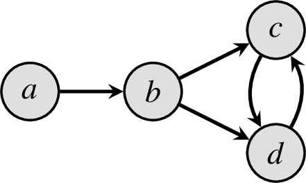
Fig. 1.
AF F with
Definition 1.
Let
Example 1.
Consider the AF
Given an AF
2.2.Abstract solvers for SAT
Most SAT solvers are based on the Davis–Putnam–Logemann–Loveland (dpll) procedure [20]. We give an abstract solver for dpll following the work of Nieuwenhuis et al. [44]. The abstract solver is described by assigning a graph to each instance of the problem, where nodes and edges represent states and transitions of the actual solver, respectively. We start with basic notation for Boolean logic.
For a Conjunctive Normal Form (CNF) formula φ (resp. a set of literals M), we denote the set of atoms occurring in φ (resp. in M) by
We now introduce an abstract procedure for deciding whether a CNF formula is satisfiable. A decision literal is a literal annotated by d, as in
Each CNF formula φ determines its dpll graph
Fig. 2.
The transition rules of
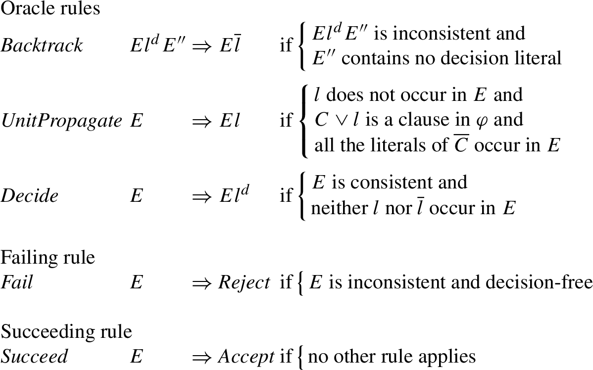
Intuitively, every state of the dpll graph represents some hypothetical state of the dpll computation whereas a path in the graph is a description of a process of search for a satisfying assignment of a given CNF formula. The rule
To decide the satisfiability of a CNF formula it is enough to find a path in
Theorem 2.1.
For any CNF formula φ, the graph
A proof of this theorem can be found in [36, Prop. 1] and (using a slightly different statement) in [44, Lemma 2.9]. The fact that
Figure 3 presents two paths in
Fig. 3.
Examples of paths in
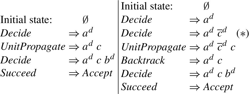
The difference between the paths in Fig. 3 is that only the path on the left will be indeed followed by SAT solvers, given it adheres with the ordering followed by SAT solvers, while the path on the right applies
2.3.Abstract solvers for computing maximal satisfying assignments
We now define a modification of the graph presented in the previous sub-section that will be useful in the definition of a new solving algorithm in Section 3.4.
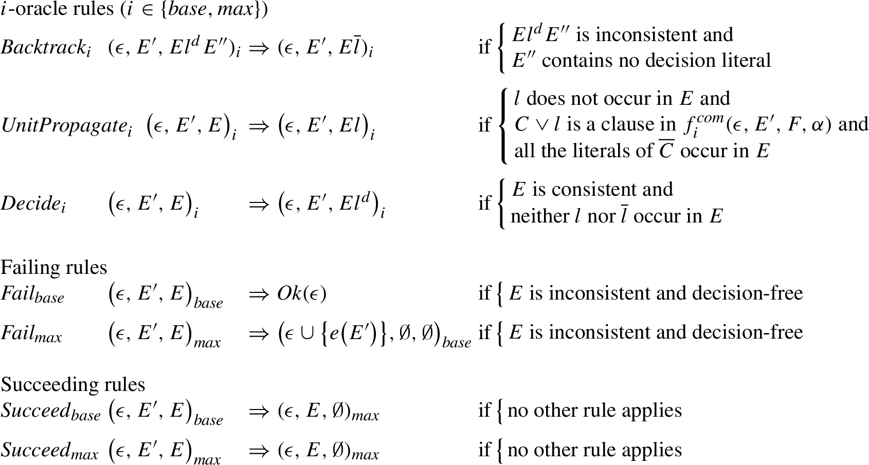
The goal of this graph is to compute a maximal satisfying assignment of a CNF formula in the sense that the set of atoms mapped to true is ⊆-maximal among all satisfying assignments. In order to do this it is enough to modify the graph
Let us call the resulting graph
Theorem 2.2.
For any CNF formula φ, the graph
Proofs of this theorem can be found in [47, Theorem 2] and in [12, Prop. 1].
3.Algorithms for preferred semantics
In this section we first abstract two SAT-based algorithms for preferred semantics, namely PrefSat [13] (implemented in the tool ArgSemSat [14]) for extension enumeration, and an algorithm for deciding skeptical acceptance of cegartix [25]. Moreover, we abstract the dedicated approach for enumeration of [45]. Finally, in Section 3.4 we show how our graph representations can be used to develop a novel algorithm, by combining parts of cegartix and
A key insight of the SAT-based algorithms is that preferred extensions can be found by iterative computation of certain extensions of a base semantics (admissible or complete): first, any extension of the base semantics is computed, and then, in each step, a strictly bigger (w.r.t. subset) one is computed. As these subproblems are in
We will present these algorithms in a uniform way via abstract solvers, abstracting from some minor tool-specific details. By presenting algorithms in such a uniform way, the relation among these algorithms becomes much clearer than by using, e.g. pseudo-code-based descriptions. In fact, common to all algorithms is a conceptual two-level architecture of computation, similar to Answer Set Programming solvers for disjunctive logic programs [6]. The lower level corresponds to a dpll-like search subprocedure, while the higher level part takes care of the specific theory and drives the overall algorithm. For PrefSat and cegartix, the subprocedures actually are delegated to a SAT solver, while the dedicated approach carries out a tailored search procedure. Such common architecture is difficult to spot by looking at the related pseudo-code descriptions, while it will be clear by employing abstract solvers.
Each algorithm uses its own data structures, and, by slight abuse of notation, for a given AF
(1) an annotated triple
(2)
(3) a distinguished state
The intended meaning of a state
The remaining states denote terminated computation:
The SAT-based algorithms construct formulas by a function f s.t.
We now define a strict partial order on states, that will be used to show acyclicity of graphs later in this section. First, we define a particular representation of records used for lexicographic comparison.
Definition 2.
Let E be a record. E can be written as
Example 2.
Consider the records
The orders on states are now defined in a way that the graphs produced by the abstract solvers presented in this section only feature edges between states
Definition 3.
Let
The strict partial order < on states is defined such that for any two states
(i)
(ii)
(iii)
(iv)
Example 3.
Consider the states
One can check that all orders on elements are transitive and irreflexive. Therefore the construction of < also ensures these properties for the order on states.
3.1.SAT-based algorithm for enumeration
PrefSat (Algorithm 1 of [13]) is a SAT-based algorithm for finding all preferred extensions of a given AF. The algorithm maintains a list of visited preferred extensions. It first searches for a complete extension not contained in previously found preferred extensions. If such an extension is found, it is iteratively extended until we reach a subset-maximal complete extension, which is a preferred extension by definition. This preferred extension is stored, and we repeat the process.
This algorithm is realized by two subprocedures that are delegated to a SAT solver. The first has to generate a complete extension not contained in one of the enumerated preferred extensions, and the second searches for a complete extension that is a strict superset of a given one.
Fig. 4.
The rules of
We now represent PrefSat as an abstract solver. The graph
In words, the models of the formula
We remark that α is not relevant for enumeration of extensions and only used for acceptance later on. In the interest of uniformity we keep it as parameter of the functions throughout the paper. Recall that in a state
As the oracle rules with annotation
Example 4.
Again consider the AF F depicted in Fig. 1. We have seen in Example 1 that F has two preferred extensions, namely
It remains to show correctness of
Lemma 3.1.
For any AF F and
We continue with a lemma stating that only preferred extensions which have not been found at this point are added to ϵ.
Lemma 3.2.
For any AF F, if the rule
Proof.
Let
Since the initial state is
Now we are ready to show correctness of
Theorem 3.3.
For any AF F, the graph
Proof.
In order to show that
In order to show that it is acyclic recall the strict partial order < on states from Definition 3. We show that each transition rule is increasing w.r.t. < by referring to the conditions (i) to (iv) from Definition 3. To this end consider two states
The only terminal state reachable from the initial state is
3.2.SAT-based algorithm for acceptance
cegartix [25] is a SAT-based tool for deciding several acceptance questions for AFs. Here we focus on Algorithm 1 of [25] for deciding skeptical acceptance w.r.t. preferred semantics of an argument α. Similarly to PrefSat, cegartix traverses the search space of a certain semantics, generates candidate extensions not contained in already visited preferred extensions, and maximizes the candidate until a preferred extension is found. The main differences to PrefSat are (1) the parametrized use of base semantics σ (the search space), which can be either admissible or complete semantics, and (2) the incorporation of the queried argument α. To prune the search space, α must not be contained in the candidate σ-extension before maximization. Again, we have two kinds of SAT-calls.
The graph
Fig. 6.
Changed transition rules for
The graph
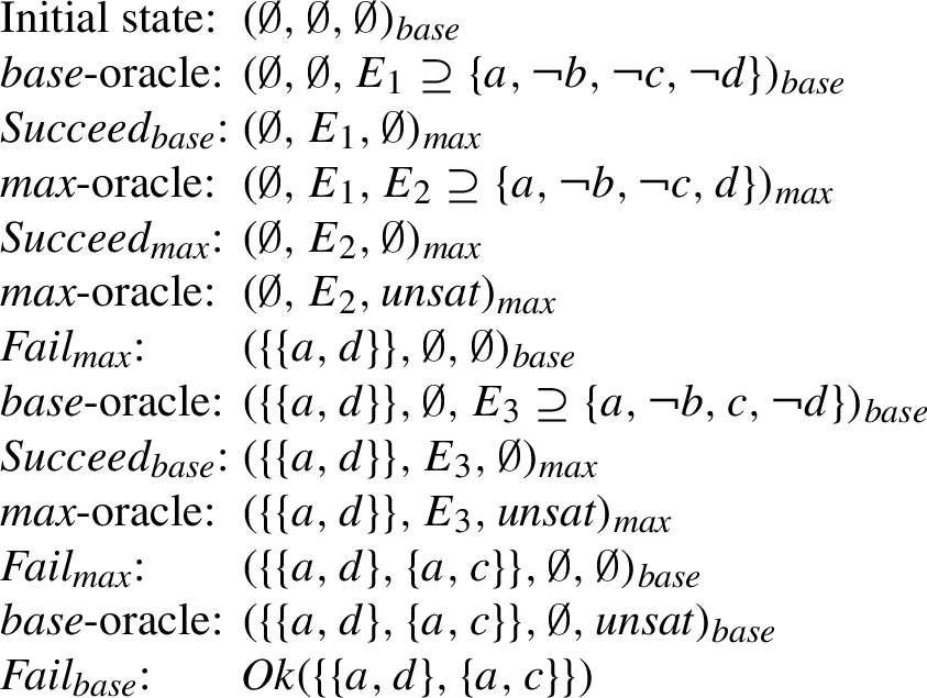
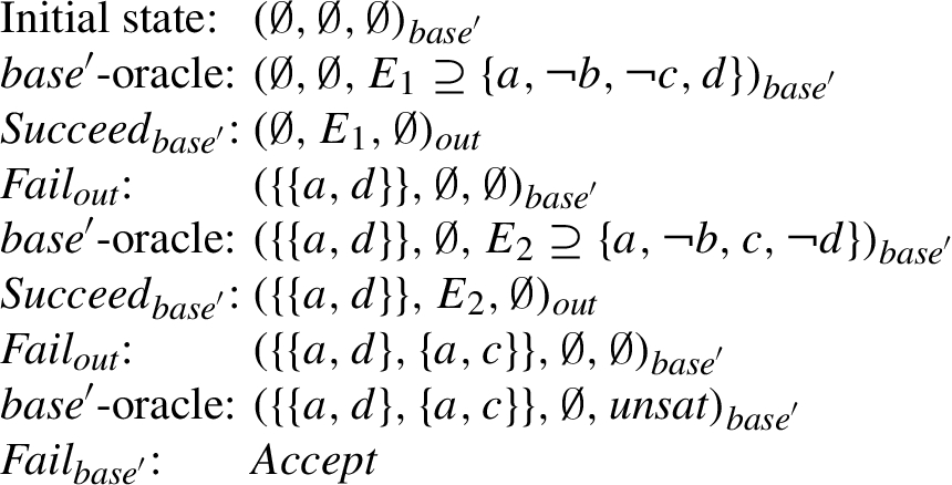
Example 5.
Again consider the AF F from Fig. 1 and note that skeptical acceptance of argument c is rejected as c is not contained in the preferred extension
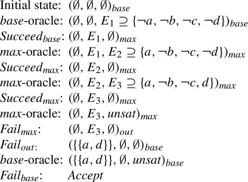
On the other hand, argument a is skeptically accepted w.r.t. preferred semantics in F as it belongs to all preferred extensions enumerated in
Fig. 7.
Reject-path for argument c in
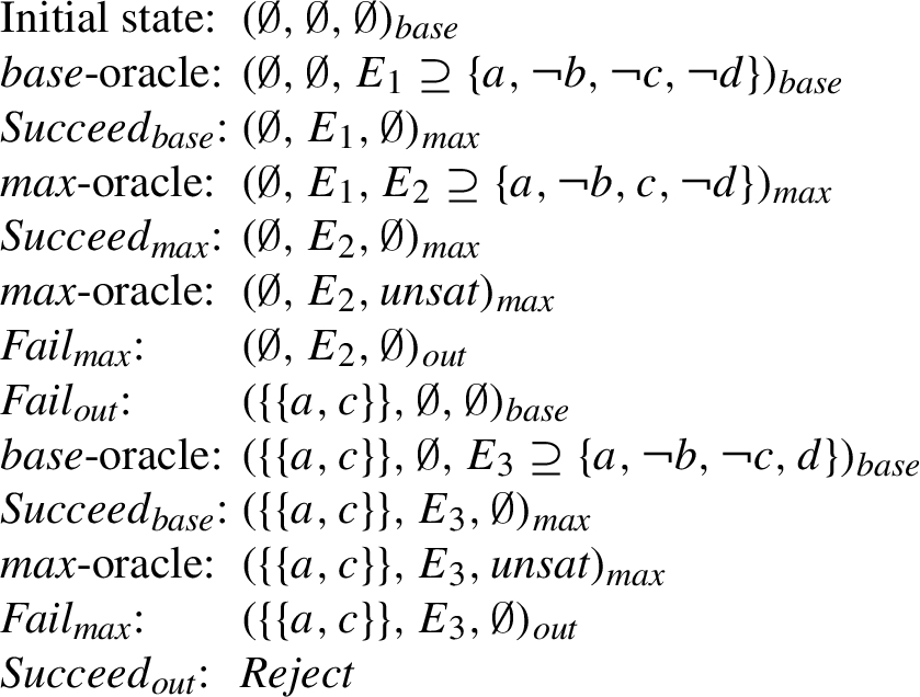
Fig. 8.
Accept-path for argument a in
Again, we get the following from Theorem 2.1:
Lemma 3.4.
For any AF
The proof of the following results is almost identical to the ones of Lemma 3.2 and Theorem 3.3 and can be found in the Appendix.
Lemma 3.5.
For any AF F, if the rule
Theorem 3.6.
For any AF
Finally note that from Theorem 3.6 it follows that
3.3.Dedicated approach for enumeration
Algorithm 1 of [45] presents a direct approach for enumerating preferred extensions. One function is important for this algorithm, which is called IN-TRANS. Given an AF
The algorithm is recursive, and stores the admissible extensions in a global variable. First, it checks whether all the arguments are marked as either belonging to or being outside the extension, and if so it returns after adding the extension to the global variable if the extension is actually admissible. Second, it applies the function IN-TRANS to some unmarked argument and calls itself recursively. Third, it reverts the effects of IN-TRANS, marks the argument it chose as outside of this extension, and calls itself recursively.
We have defined an equivalent representation of this algorithm that follows the framework of abstract solvers with binary logics as previously used in this article. Binary truth values are sufficient to represent the arguments marked, but we see the labels “attacked” and “to be attacked” as an optimization as they can be easily recovered at the end of the algorithm. Indeed, they correspond to the condition “there is an argument a such that
Fig. 9.
The rules of the graph
The graph
More precisely, among the oracle rules, propagation (through
A final comment is related to one of the main advantages of using abstract solvers, i.e. the fact that they allow to highlight in a more clear way similarities and differences among solving algorithms, as mentioned in Section 1. It is evident that our reformulation of the direct approach has allowed to present this algorithm by modification of the previous two solving procedures, by explicitly viewing it in the light of a backtrack-search process in a search space, more similar to a SAT-based procedure. This would not be obvious by considering, e.g. the pseudo-code description of the direct approach.
Example 6.
A possible path in the graph
We give the correctness statement of the abstract solver representing the direct approach after providing an intermediate lemma; proofs can again be found in the Appendix.
Lemma 3.7.
For any AF F, if the rule
Theorem 3.8.
For any AF F, the graph
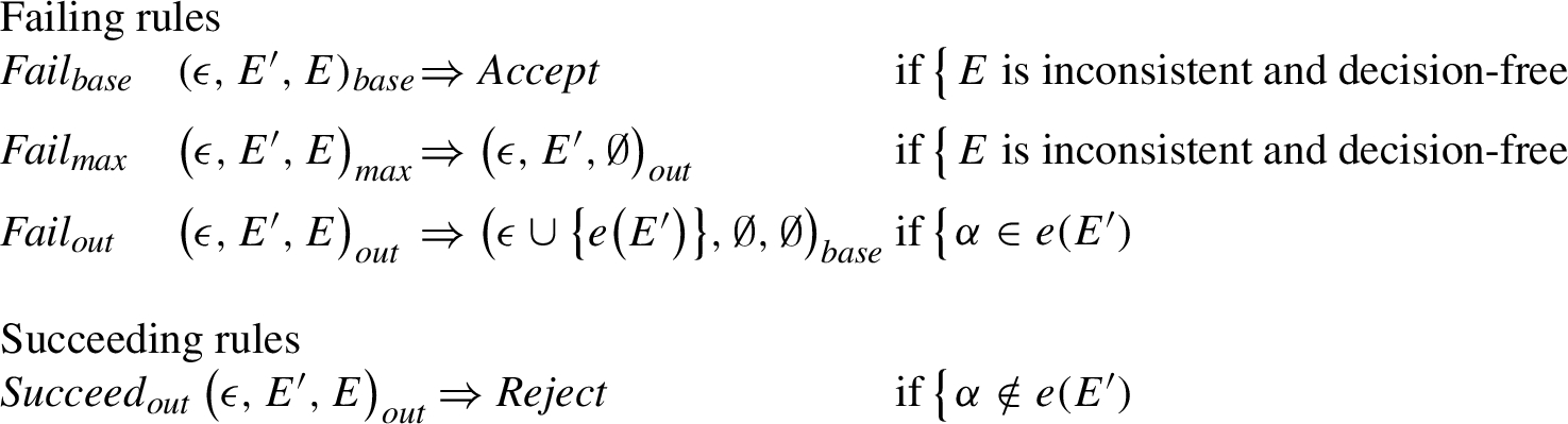
3.4.Combining algorithms
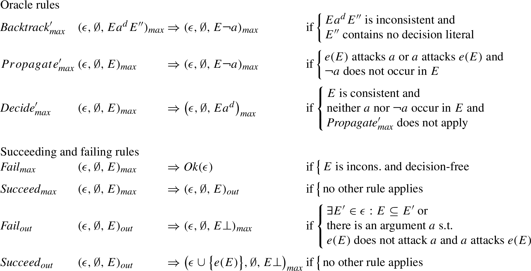
We now use the insights gained by the graph representations of the algorithms from the literature to define a new algorithm for skeptical acceptance w.r.t. preferred semantics. We do so by defining a new abstract solver which incorporates the modified dpll (cf. Section 2.3) into the graph representation of cegartix (cf. Section 3.2). This gives rise to a new algorithm which is not only of theoretical interest, but also leads to a more efficient solving procedure, as we will show in Section 4.
Now recall that, in PrefSat and cegartix, the two SAT calls annotated with
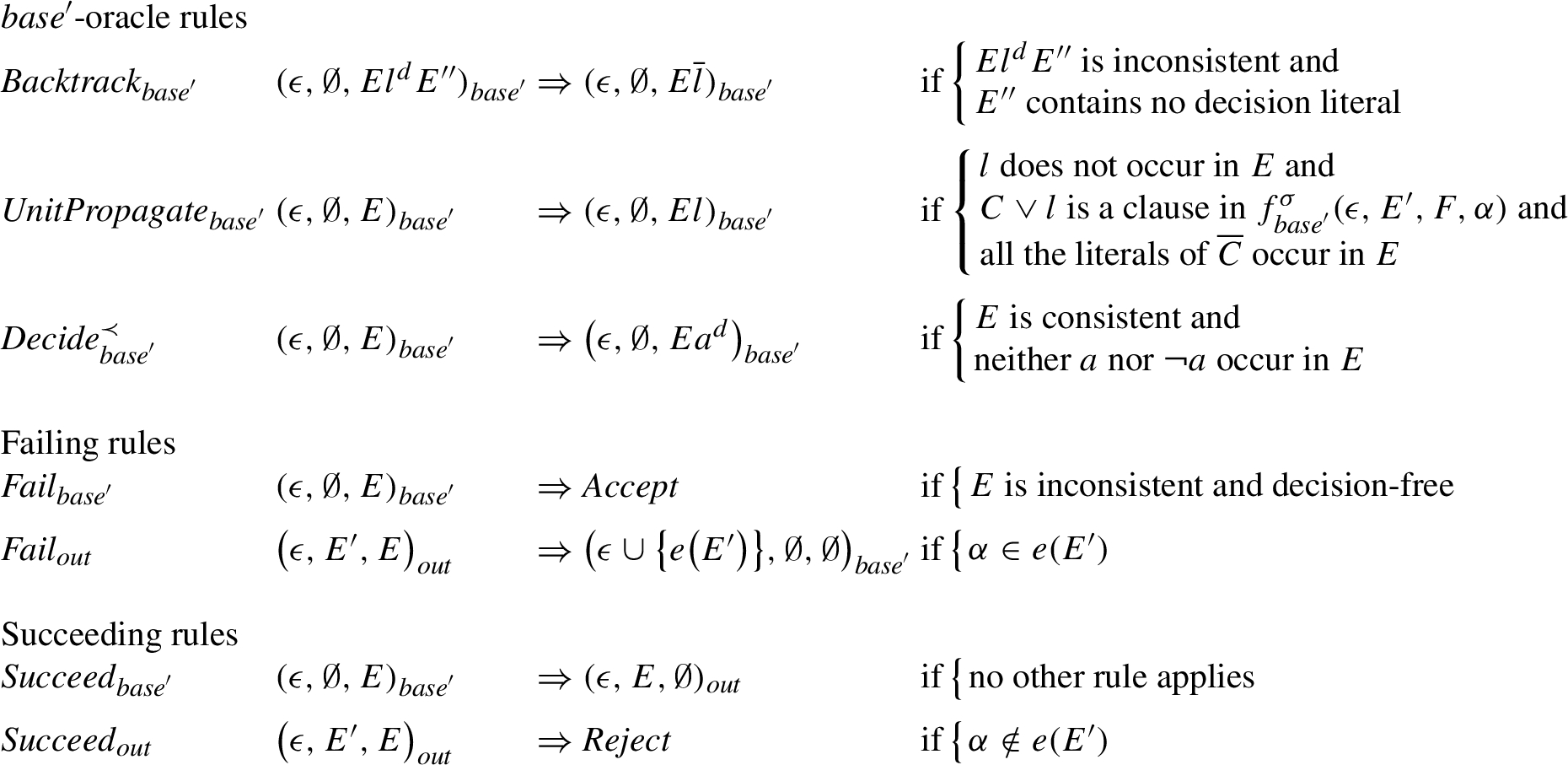
But, given our result in Section 2.3, the “inner loop” of SAT calls for maximization is not strictly needed, and the two types of SAT calls can be substituted by a single modified call. More specifically, we replace
Given an AF F, an argument α and a base semantics
Then, the outcome of the
Fig. 11.
The rules of
Considering the fact that the new solution always adds positive atoms to the current assignment, it looks similar to the direct approach; but there is a notable difference between the new algorithm and the direct approach. The outcome of the oracle-rules of the direct approach (cf. Fig. 9) is a conflict-free set which is not necessarily maximal (and in other rules admissibility and maximality is checked), whereas the outcome of the oracle-rules in the new algorithm modifying
From Theorem 2.2 we know that the
Lemma 3.9.
For any AF
To be sure that maximal satisfying assignments correspond to preferred extensions, it has to hold that the atoms occurring in
Assumption 1.
Given an AF
It is important to note that the concrete formulas used in cegartix fulfill Assumption 1. Taking the assumption for granted in the rest of the paper, we are able to show correctness of the abstract solver representing the combined approach.
Lemma 3.10.
For any AF F, if the rule
Theorem 3.11.
For any AF
Proof.
(1)
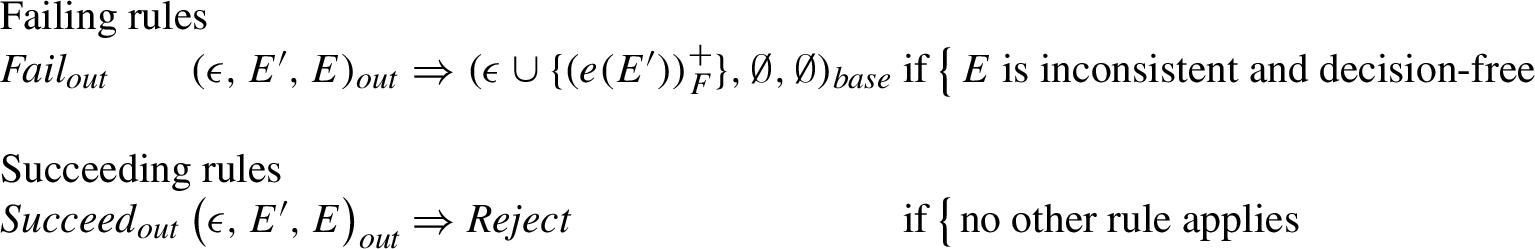
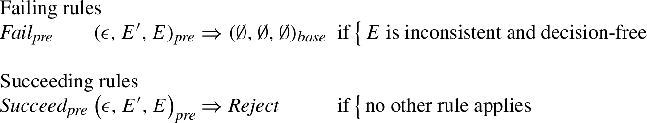
(2) Any terminal state of
(3)
(⇒): Assume
(⇐): Assume α is not skeptically accepted by F w.r.t.
Again it is important to note that from Theorem 3.11 it follows that
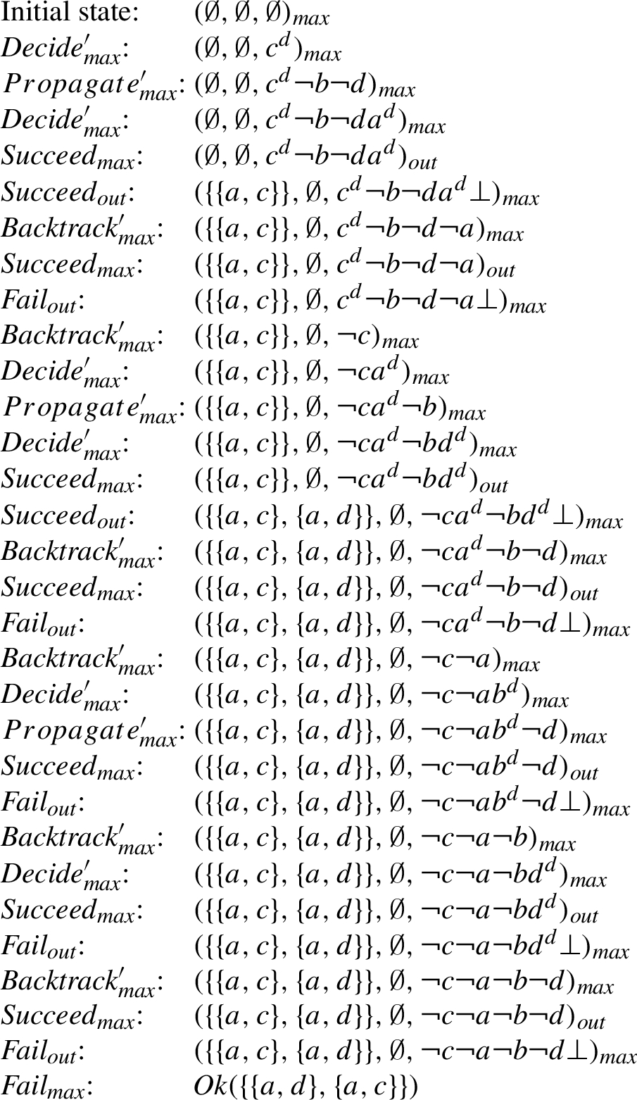
Fig. 12.
Reject-path for argument c in
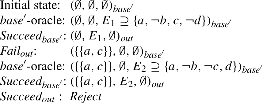
Fig. 13.
Accept-path for argument a in
Example 7.
For the AF F from Fig. 1, a possible path in
Of course, in principle it is not clear whether the new abstract solution leads to computational advantages (see, e.g. [30,31] for a related discussion); however, the experimental analysis in Section 4 shows that this is the case.
4.Experiments
In order to test the viability of our proposed combination as introduced in Section 3.4, we have implemented an alternative version of cegartix following the new approach. The choice of cegartix is motivated by the fact that it has been one of the best AF solvers in both editions of the argumentation competition (http://argumentationcompetition.org). In particular, in the reasoning task of interest (skeptical acceptance under preferred semantics as in Section 3.2), cegartix was 2nd out of 11 solvers entering the track in the first competition, and highly competitive also in the second event.33
4.1.Implementation
The main change done in cegartix was thus replacing the two inner SAT calls with a single call to a SAT solver with modified heuristics, and we obtained this by changing the internal heuristics of the clasp solver used by cegartix in the 2015 competition. clasp [29] is an ASP solver, but can act also as SAT solver with excellent results as shown in past SAT competitions, starting from 2009 to the most recent editions (see, e.g. http://www.satcompetition.org/). Moreover, for efficiency reasons, the implementation of cegartix slightly differs from the algorithm in Section 3.2, given that the condition
The variants of cegartix considered in our experiments are:
(1) ceg: version with com as a base semantics, which was the setting employed in both editions of the competition. Past experiments ([25], on different benchmark graphs) overall showed similar or better performance of this version compared to that with adm as a base semantics.
(2) ceg+-com: new version implementing the combination in Section 3.4 with com as a base semantics.
(3) ceg+-adm: new version implementing the combination in Section 3.4 with adm as a base semantics.
The version of cegartix entering the competition included shortcuts, i.e. specific conditions that can lead the solver to find solutions earlier, before entering the main solving algorithm. Details for shortcuts will be presented in the next section. For this analysis, given the main goal is to test the new solution which applies to the core part of the algorithm and shortcuts could obfuscate the differences between algorithms, shortcuts have been disabled. Note, however, that the new variants can make use of the very same shortcuts. Therefore, it has to be noted that final implementations of the respective algorithms might show smaller gaps in performance, since they will all use the same shortcuts in the first place.
4.2.Benchmarks
For benchmarks, i.e., instances comprising of an AF and an argument for which one has to check skeptical acceptance under preferred semantics, we considered the following three benchmark sets44
ICCMA’15: These are 192 AFs with three arguments to be queried for, from the competition in the year 2015 [50]. After cleaning this dataset from trivial queries (queried arguments not among the set of arguments in the AF), this resulted in 537 instances.
ICCMA’17: In this dataset, from the competition in the year 2017 [27], we have 300 AFs, divided into four categories (according to expected difficulty), which were used to compare solvers for the task of checking skeptical acceptance under preferred semantics (this set is called set “A” in the competition). The hardest category has two arguments to be queried for per AF, while all other three categories have one query argument. This results in 350 instances.
CLIMA: This is a set of AFs from our earlier work [53], which we included since it comprises of several AFs that were hard to solve by an earlier version of cegartix. Here we have 320 AFs and one query argument per AF. The AFs
4.3.Results
Experiments have been run on an AMD Opteron Processor 6308 3.5 GHz with 2 processors with each 2 physical cores; every of these cores puts at disposal 2 logical cores, for a sum of 192 GB (
We first show general runtime statistics in Table 1. More concretely, the table depicts median runtimes over the considered benchmark sets, as well as timeouts encountered in the runs. The last two columns list the number of instances that were uniquely solved by ceg or by the union of solved instances of ceg+-com and ceg+-adm, i.e., whether the original approach or the new approaches could contribute to uniquely solved instances.
Table 1
General runtime statistics from experiments
| Median runtime | Timeouts | Uniquely solved | ||||||
| Benchmark | ceg | ceg+-com | ceg+-adm | ceg | ceg+-com | ceg+-adm | by ceg | by ceg+-com or ceg+-adm |
| All | 1.01 | 1.14 | 1.28 | 57 | 61 | 71 | 6 | 11 |
| ICCMA’15 | 0.77 | 0.93 | 0.76 | 0 | 0 | 0 | 0 | 0 |
| ICCMA’17 | 9.75 | 7.96 | 23.30 | 45 | 47 | 60 | 5 | 8 |
| CLIMA | 1.04 | 1.1 | 0.99 | 12 | 14 | 11 | 1 | 3 |
This table indicates that, regarding median runtime and timeouts, the new approaches generally do not fare (much) better than the original version of cegartix. In fact, median runtimes and timeouts overall increased when comparing new and original approaches, except for median running time of ceg+-com on benchmark ICCMA’17 and, to a small extent, ceg+-adm on benchmark CLIMA. A further observation is that the instances from benchmark ICCMA’15 are rather easy to solve.
Nevertheless, the uniquely solved instances indicate differences of the approaches w.r.t. runtime performance. Looking closer at these uniquely solved instances, when ceg+-com or ceg+-adm could solve an instance within the timeout limit and ceg could not, it was always the case that ceg+-adm solved the instance, while this was only sometimes the case for ceg+-com. That is, ceg+-adm contributes to all of the uniquely solved instances, while ceg+-com only to five of the eleven instances.
We next illustrate, via Fig. 14, the different runtime behaviors of the three cegartix implementations via scatter plots. In Fig. 14(a), the scatter plot between ceg and ceg+-adm is shown, while in Fig. 14(b), ceg is compared to ceg+-com and, finally, in Fig. 14(c), the scatter plot of the two new solvers is shown. Such plots show the running time of two solvers (on x and y axes) on each individual instance. A runtime directly on the diagonal implies the same runtime for both solvers on that instance.
Closer inspection of the figures suggests that the solver ceg and the two solvers ceg+-com and ceg+-adm are rather complementary in their runtime behavior on many (non-easy) instances. That is, apart from the uniquely solved instances (these are the ones on the “timeout” lines for one of the solvers), also several further instances showed different runtime behavior: in both Fig. 14(a) and Fig. 14(b) several instances can be seen below or above the diagonal.
Fig. 14.
Scatter plots of our experimental analysis. Black circles indicate instances with an AF that has an empty grounded extension, while a red cross indicates a non-empty grounded extension.
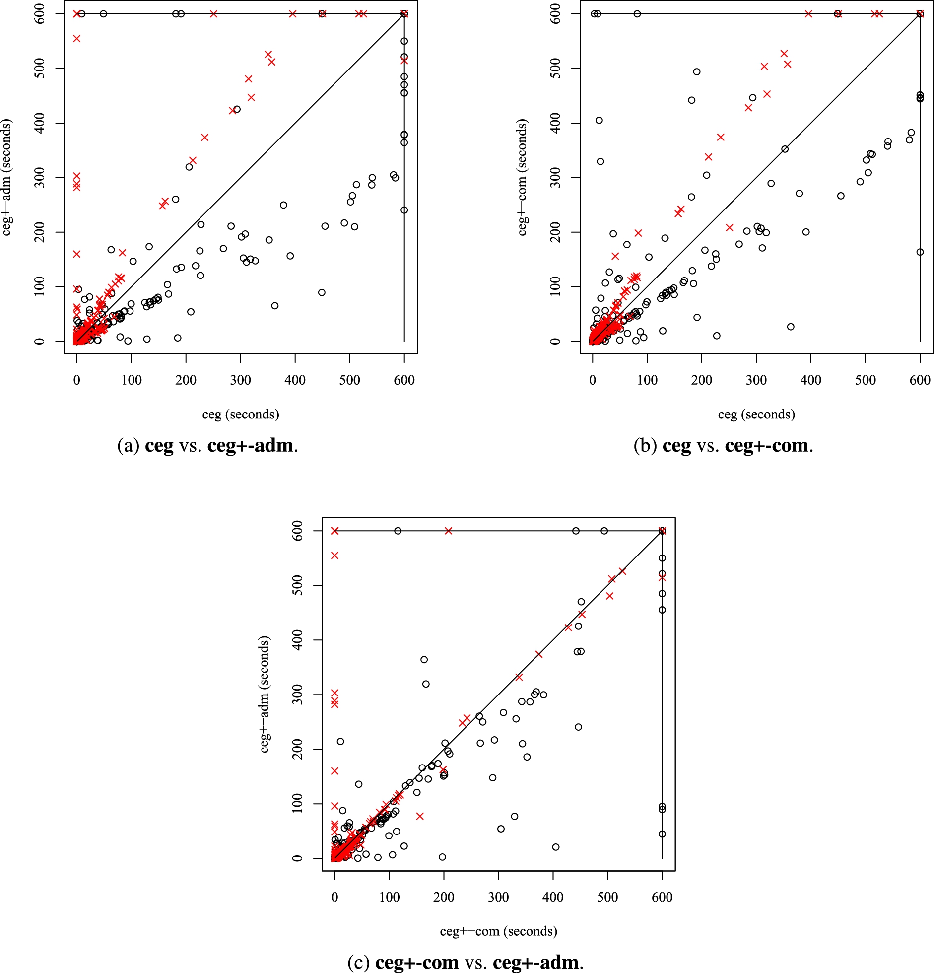
We hypothesize that a reason for the different runtimes, for original ceg and novel ceg+-com and ceg+-adm, stems from difficulties of ceg to find non-trivial (i.e., non-empty) admissible sets. To investigate towards this end, we have marked each instance of each scatter plot, in Figs 14(a)–(c), whether the corresponding AF has a non-empty grounded extension or not. When an AF has an empty grounded extension the corresponding symbol in the figure is a black circle, otherwise a red cross. An AF having a non-empty grounded extension can be seen as a kind of approximation of whether one can (easily) find a non-trivial admissible set. In Fig. 14(a) and Fig. 14(b), this categorization of the instances is, to some extent, reflected in the runtimes: many times when a novel solver outperformed ceg it is the case when the grounded extension is empty. When looking at Fig. 14(c), comparing running times of ceg+-com and ceg+-adm, the results suggest that on AFs with an empty grounded extension, ceg+-adm tends to be better w.r.t. running time, yet on AFs with a non-empty grounded extension, many instances, on that figure, are either in the diagonal or, in fact, trivial for ceg+-com, but not for ceg+-adm.
Although further research is needed, the characteristic of an AF having a (non-)empty grounded extension gives an indicator whether ceg or ceg+-com and ceg+-adm might be better to use for solving. This insight can be used, for instance, when compiling an algorithm selection for cegartix, in line with techniques studied in [15], to first compute the grounded extension, and then choose which heuristic to apply.
5.Extensions to the framework
In Section 3 we have analyzed three prominent algorithms from the literature dealing with preferred semantics. In this section we show that the modularity of the abstract solver approach allows us to give the graph representation of related algorithms with little effort. First, we abstract the algorithms from [25] deciding skeptical (resp. credulous) acceptance w.r.t. other, namely stage [52] and semi-stable [11], semantics, and then we exemplify how to incorporate shortcuts into the graph-representations for the algorithms of the same paper.
5.1.Core algorithms for semi-stable and stage semantics
Other semantics involving reasoning tasks lying in the second level of the polynomial hierarchy are stage and semi-stable (cf. Table 2). Their definitions make use of the concept of the range of a set of arguments
Definition 4.
Given an AF F,
Table 2
Complexity of decision problems for AFs
| σ | ||
For semi-stable semantics the possible base semantics coincide with the ones for preferred semantics, that is admissible and complete, while stage semantics (yielding range-maximal conflict-free sets) uses conflict-free as base semantics. In other words, for the pairs
Algorithms for skeptical (resp. credulous) acceptance w.r.t. these semantics are presented in Algorithms 2 and 3 of [25] by adaptation of the algorithm for skeptical acceptance w.r.t. preferred semantics described in Section 3.2. Similar to the algorithm for preferred semantics, the general skeptical acceptance procedure for semantics θ and base semantics σ first makes use of two SAT oracles to find a range-maximal σ-extension. The main difference to the algorithm for preferred semantics is that the maximization is concerned with the range of extensions instead of the extensions themselves. Moreover, since there can be different σ-extensions with the same range, another oracle has to be consulted in order to check whether there is a σ-extension with a range equal to the maximal one found before, which does not contain the queried argument. If such an extension exists, the algorithm returns with a negative answer to the skeptical acceptance problem w.r.t. θ. For credulous acceptance, the algorithm returns with a positive answer if the oracle call finds such a σ-extension which does contain the queried argument.
The graph
Fig. 15.
The transition rules of the graph
The initial state of
Functions
Likewise, the graph
The following results show correctness of the abstract solvers for acceptance problems w.r.t. semi-stable and stage semantics described in this section. The proofs, which follow the same structure as previous proofs, can be found in the Appendix.
Lemma 5.1.
For
Theorem 5.2.
For
Finally note again that from Theorem 5.2 it follows that
5.2.Shortcuts for cegartix-algorithms
When defining abstract solvers for the algorithms of cegartix in previous sections we restricted our attention to the core of the algorithm. In this section we show that the graphs presented so far can be easily extended in a modular way to capture the full algorithms.
We do so by abstracting the full Algorithm 1 of [25] for skeptical acceptance w.r.t. preferred semantics, including the shortcut computation performed at the beginning of the algorithm. By this shortcut, the algorithm immediately returns with a negative answer for the skeptical acceptance problem w.r.t. preferred semantics, if there is a σ-extension (
We add the transition rules presented in Fig. 16.
Moreover, there is a set of oracle rules with index
The initial state is
Fig. 16.
The transition rules of the graph
Theorem 5.3.
For any AF
6.Related work
The use of abstract solvers was initiated by Nieuwenhuis et al. [44]. In that work the authors first presented an abstract solver for SAT, similar to our introduction of abstract solvers in Section 2.2. Then, they presented two extensions: (i) a description of Conflict-Driven Clause Learning SAT solving, i.e. involving backjumping and learning techniques, by means of modular addition of transition rules, but also by changing the definition of states to account for learned clauses, and (ii) they considered also Satisfiability Modulo Theories (SMT) problems with certain logics via a lazy approach [48], i.e. where the SAT calls are made to provide satisfying assignments of the Boolean abstraction of the SMT problem that are then checked for “SMT consistency”. Lierler [35] imported this methodology to Answer Set Programming (ASP), by first designing abstract solvers for some backtracking-based ASP solvers for non-disjunctive ASP solving, and then enhancing her approach to include backjumping and learning techniques [36]. Another extension for describing CASP solvers, i.e. systems able to deal with a combination of ASP and constraint programming, a language useful to represent and reason on hybrid domains, has been put forward in [37]. Other works on abstract solvers are [38], where solvers for different formalisms, e.g. ASP and SAT with Inductive Definitions, are compared by means of comparison of the related graphs, and the following series of papers where, starting from a developed concept of modularity in answer set solving [39], abstract modeling of solvers for multi-logic systems are presented [40–42].
If we turn our attention to the usage of abstract solvers for dealing with reasoning tasks beyond NP, the situation is less developed and only very recently few works have been put forward. Abstract solvers for certain disjunctive answer set solvers implementing basic backtracking have been introduced by Brochenin et al. [6] and are studied in a more general way in [7]. Even more recently, abstract solvers for satisfiability of Quantified Boolean Formulas [9] and cautious reasoning in ASP [10] have been presented.
Only few of the aforementioned works [36,44] have already aimed for the implementation of combinations of algorithms based on abstract solvers; thus, our practical results are particularly remarkable.
As far as other algorithms for the preferred semantics in the literature are concerned, we mention [22,43], where a labelling-based approach is employed. These algorithms differ in the initial labellings and how transitions are applied to argument labels. Moreover, [43] includes other semantics than preferred and also argument-based proof theories, another way to characterize an algorithm’s behavior but whose goal is not to be the basis for an implementation.
The argumentation solver competition 2015 [51] had eleven participating systems in the task of deciding skeptical acceptance of an argument w.r.t. preferred semantics. The first two places were taken by ArgSemSAT and cegartix, whose algorithms are described in terms of abstract solvers in Sections 3.1 and 3.2, respectively. The other solvers in the top five were LabSATSolver, ASPARTIX-V [28] and CoQuiAAS [32] (system descriptions of all participating solvers can be found in [49]). While LabSATSolver uses the same algorithm as ArgSemSAT for this particular task, ASPARTIX-V and CoQuiAAS are reduction-based approaches, using translations to ASP and a particular variant of Max-SAT, respectively. Thus, being based on reduction, their modeling via abstract solvers is less interesting for the abstract argumentation community, given that this would boil down to modeling, respectively, ASP and Max-SAT search algorithms. For this reason, they have not been considered in this paper.
7.Conclusions
In this paper we have shown the applicability and the advantages of using a rigorous formal way for describing certain algorithms for solving decision problems for abstract argumentation frameworks through graph-based abstract solvers instead of, e.g. pseudo-code-based descriptions. Both SAT-based and dedicated approaches for solving hard problems have been analyzed and compared, with focus on algorithms for the preferred semantics. Moreover, by combining abstract solvers, we have obtained a novel algorithm for skeptical acceptance. The algorithm has been implemented taking cegartix [25] as a starting point. An experimental analysis on the benchmark graphs of the first and second argumentation competition, as well as on graphs from earlier work, shows that the new algorithm is complementary to an existing algorithm in cegartix. The above analysis has focused, as said, on the well-studied preferred semantics, and on core algorithms. We have then shown how the machinery can be employed to describe algorithms for different semantics, e.g. semi-stable and stage semantics, as employed in cegartix, and for taking into account specific optimization techniques by means of modular addition of transition rules to the graphs describing the core parts of the algorithms.
As future work, we want to apply the concept of abstract solvers to other promising algorithms and optimization techniques for reasoning tasks in abstract argumentation. In particular, we plan to study certain approaches to the decomposition of AFs [2,16,33,34]. Moreover, we plan to extend our experimental analysis for the new version of cegartix by studying on which classes of AFs the new version is performing better than existing algorithms.
Notes
1 In the literature also infinite AFs have been considered. We refer to [3] for the effects this has on semantics.
2 The class
4 Archives of the benchmark sets can be found at http://argumentationcompetition.org/2015/iccma2015_benchmarks.zip, http://www.dbai.tuwien.ac.at/iccma17/benchmarks/A.tar.gz, and http://www.dbai.tuwien.ac.at/research/project/argumentation/cegartix/files/clima.zip.
Acknowledgements
We thank Benjamin Kaufmann, member of the Potassco team, for suggesting how to modify the version of clasp employed in the experiments. This work has been funded by the Austrian Science Fund (FWF) through projects I1102, I2854 and P30168-N31, and by Academy of Finland through grants 251170 COIN and 284591.
Appendices
Appendix
AppendixProofs
Proof of Lemma 3.5.
Let
Since the initial state is
Proof of Theorem 3.6.
(1)
(2) Any terminal state of
(3)
Proof of Lemma 3.7.
The application of
Proof of Theorem 3.8.
Since states of
To show that
(i)
(ii)
(iii)
The only terminal state reachable from the initial state is
Proof of Lemma 3.10.
Let
Proof of Lemma 5.1.
Let
Since the initial state is
Proof of Theorem 5.2.
We show the result for
(1)
(2) Any terminal state of
(3)
Proof of Theorem 5.3.
Finiteness is inherited from
A
Since the shortcut can only reject instances it follows from Theorem 3.6 that if
References
[1] | P. Baroni, M.W.A. Caminada and M. Giacomin, An introduction to argumentation semantics, The Knowledge Engineering Review 26: (4) ((2011) ), 365–410. doi:10.1017/S0269888911000166. |
[2] | R. Baumann, Splitting an argumentation framework, in: Proceedings of the 11th International Conference on Logic Programming and Nonmonotonic Reasoning, LPNMR 2011, J.P. Delgrande and W. Faber, eds, Lecture Notes in Computer Science, Vol. 6645: , Springer, (2011) , pp. 40–53. |
[3] | R. Baumann and C. Spanring, Infinite argumentation frameworks – On the existence and uniqueness of extensions, in: Advances in Knowledge Representation, Logic Programming, and Abstract Argumentation – Essays Dedicated to Gerhard Brewka on the Occasion of His 60th Birthday, T. Eiter, H. Strass, M. Truszczynski and S. Woltran, eds, Lecture Notes in Computer Science, Vol. 9060: , Springer, (2015) , pp. 281–295. |
[4] | T.J.M. Bench-Capon and P.E. Dunne, Argumentation in artificial intelligence, Artificial Intelligence 171: (10–15) ((2007) ), 619–641. doi:10.1016/j.artint.2007.05.001. |
[5] | P. Besnard and S. Doutre, Checking the acceptability of a set of arguments, in: Proceedings of the 10th International Workshop on Non-Monotonic Reasoning, NMR 2004, J.P. Delgrande and T. Schaub, eds, (2004) , pp. 59–64. |
[6] | R. Brochenin, Y. Lierler and M. Maratea, Abstract disjunctive answer set solvers, in: Proceedings of the 21st European Conference on Artificial Intelligence, ECAI 2014, T. Schaub, G. Friedrich and B. O’Sullivan, eds, Frontiers in Artificial Intelligence and Applications, Vol. 263: , IOS Press, (2014) , pp. 165–170. |
[7] | R. Brochenin, Y. Lierler and M. Maratea, Disjunctive answer set solvers via templates, Theory and Practice of Logic Programming 16: (4) ((2016) ), 465–497. doi:10.1017/S1471068415000411. |
[8] | R. Brochenin, T. Linsbichler, M. Maratea, J.P. Wallner and S. Woltran, Abstract solvers for Dung’s argumentation frameworks, in: Proceedings of the 3rd International Workshop on Theory and Applications of Formal Argumentation, TAFA 2015, Revised Selected Papers, E. Black, S. Modgil and N. Oren, eds, Lecture Notes in Computer Science, Vol. 9524: , Springer, (2015) , pp. 40–58. |
[9] | R. Brochenin and M. Maratea, Abstract solvers for quantified Boolean formulas and their applications, in: Proceedings of the 14th International Conference of the Italian Association for Artificial Intelligence, AI*IA 2015, M. Gavanelli, E. Lamma and F. Riguzzi, eds, Lecture Notes in Computer Science, Vol. 9336: , Springer, (2015) , pp. 205–217. |
[10] | R. Brochenin and M. Maratea, Abstract answer set solvers for cautious reasoning, in: Proceedings of the Technical Communications of the 31st International Conference on Logic Programming, ICLP 2015, M.D. Vos, T. Eiter, Y. Lierler and F. Toni, eds, CEUR Workshop Proceedings, Vol. 1433: , CEUR-WS.org, (2015) . |
[11] | M. Caminada, W. Carnielli and P.E. Dunne, Semi-stable semantics, Journal of Logic and Computation 22: (5) ((2012) ), 1207–1254. doi:10.1093/logcom/exr033. |
[12] | T. Castell, C. Cayrol, M. Cayrol and D.L. Berre, Using the Davis and Putnam procedure for an efficient computation of preferred models, in: Proceedings of the 12th European Conference on Artificial Intelligence, ECAI 1996, W. Wahlster, ed., Wiley, Chichester, (1996) , pp. 350–354. |
[13] | F. Cerutti, P.E. Dunne, M. Giacomin and M. Vallati, Computing preferred extensions in abstract argumentation: A SAT-based approach, in: Proceedings of the 2nd International Workshop on Theory and Applications of Formal Argumentation, TAFA 2013, Revised Selected Papers, E. Black, S. Modgil and N. Oren, eds, Lecture Notes in Computer Science, Vol. 8306: , Springer, (2014) , pp. 176–193. |
[14] | F. Cerutti, M. Giacomin and M. Vallati, ArgSemSAT: Solving argumentation problems using SAT, in: Proceedings of the 5th International Conference on Computational Models of Argument, COMMA 2014, S. Parsons, N. Oren, C. Reed and F. Cerutti, eds, Frontiers in Artificial Intelligence and Applications, Vol. 266: , IOS Press, (2014) , pp. 455–456. |
[15] | F. Cerutti, M. Giacomin and M. Vallati, Algorithm selection for preferred extensions enumeration, in: Proceedings of the 5th International Conference on Computational Models of Argument, COMMA 2014, S. Parsons, N. Oren, C. Reed and F. Cerutti, eds, Frontiers in Artificial Intelligence and Applications, Vol. 266: , IOS Press, (2014) , pp. 221–232. |
[16] | F. Cerutti, M. Giacomin, M. Vallati and M. Zanella, An SCC recursive meta-algorithm for computing preferred labellings in abstract argumentation, in: Proceedings of the 14th International Conference on Principles of Knowledge Representation and Reasoning, KR 2014, C. Baral, G.D. Giacomo and T. Eiter, eds, AAAI Press, (2014) , pp. 42–51. |
[17] | F. Cerutti, N. Oren, H. Strass, M. Thimm and M. Vallati, A benchmark framework for a computational argumentation competition, in: Proceedings of the 5th International Conference on Computational Models of Argument, COMMA 2014, S. Parsons, N. Oren, C. Reed and F. Cerutti, eds, Frontiers in Artificial Intelligence and Applications, Vol. 266: , IOS Press, (2014) , pp. 459–460. |
[18] | F. Cerutti, M. Vallati and M. Giacomin, Where are we now? State of the art and future trends of solvers for hard argumentation problems, in: Computational Models of Argument – Proceedings of COMMA 2016, P. Baroni, T.F. Gordon, T. Scheffler and M. Stede, eds, Frontiers in Artificial Intelligence and Applications, Vol. 287: , IOS Press, (2016) , pp. 207–218. |
[19] | G. Charwat, W. Dvořák, S.A. Gaggl, J.P. Wallner and S. Woltran, Methods for solving reasoning problems in abstract argumentation – A survey, Artificial Intelligence 220: ((2015) ), 28–63. doi:10.1016/j.artint.2014.11.008. |
[20] | M. Davis, G. Logemann and D. Loveland, A machine program for theorem proving, Communications of the ACM 5: (7) ((1962) ), 394–397. doi:10.1145/368273.368557. |
[21] | Y. Dimopoulos and A. Torres, Graph theoretical structures in logic programs and default theories, Theoretical Computer Science 170: (1–2) ((1996) ), 209–244. doi:10.1016/S0304-3975(96)80707-9. |
[22] | S. Doutre and J. Mengin, Preferred extensions of argumentation frameworks: Query answering and computation, in: Proceedings of the 1st International Joint Conference on Automated Reasoning, IJCAR 2001, R. Goré, A. Leitsch and T. Nipkow, eds, Lecture Notes in Computer Science, Vol. 2083: , Springer, (2001) , pp. 272–288. |
[23] | P.M. Dung, On the acceptability of arguments and its fundamental role in nonmonotonic reasoning, logic programming and n-person games, Artificial Intelligence 77: (2) ((1995) ), 321–358. doi:10.1016/0004-3702(94)00041-X. |
[24] | P.E. Dunne and T.J.M. Bench-Capon, Coherence in finite argument systems, Artificial Intelligence 141: (1/2) ((2002) ), 187–203. doi:10.1016/S0004-3702(02)00261-8. |
[25] | W. Dvořák, M. Järvisalo, J.P. Wallner and S. Woltran, Complexity-sensitive decision procedures for abstract argumentation, Artificial Intelligence 206: ((2014) ), 53–78. doi:10.1016/j.artint.2013.10.001. |
[26] | W. Dvořák and S. Woltran, Complexity of semi-stable and stage semantics in argumentation frameworks, Information Processing Letters 110: (11) ((2010) ), 425–430. doi:10.1016/j.ipl.2010.04.005. |
[27] | S.A. Gaggl, T. Linsbichler, M. Maratea and S. Woltran, Introducing the second international competition on computational models of argumentation, in: Proceedings of the 1st International Workshop on Systems and Algorithms for Formal Argumentation (SAFA 2016), M. Thimm, F. Cerutti, H. Strass and M. Vallati, eds, (2016) , pp. 4–9. https://www.dbai.tuwien.ac.at/iccma17/Introducing_ICCMA17.pdf. |
[28] | S.A. Gaggl, N. Manthey, A. Ronca, J.P. Wallner and S. Woltran, Improved answer-set programming encodings for abstract argumentation, Theory and Practice of Logic Programming 15: (4–5) ((2015) ), 434–448. doi:10.1017/S1471068415000149. |
[29] | M. Gebser, B. Kaufmann and T. Schaub, Conflict-driven answer set solving: From theory to practice, Artificial Intelligence 187: ((2012) ), 52–89. doi:10.1016/j.artint.2012.04.001. |
[30] | M. Järvisalo and T.A. Junttila, Limitations of restricted branching in clause learning, Constraints 14: (3) ((2009) ), 325–356. doi:10.1007/s10601-008-9062-z. |
[31] | M. Järvisalo and I. Niemelä, The effect of structural branching on the efficiency of clause learning SAT solving: An experimental study, Journal of Algorithms 63: (1–3) ((2008) ), 90–113. doi:10.1016/j.jalgor.2008.02.005. |
[32] | J. Lagniez, E. Lonca and J. Mailly, CoQuiAAS: A constraint-based quick abstract argumentation solver, in: Proceedings of the 27th IEEE International Conference on Tools with Artificial Intelligence, ICTAI 2015, IEEE Computer Society, (2015) , pp. 928–935. |
[33] | B. Liao, Toward incremental computation of argumentation semantics: A decomposition-based approach, Annals of Mathematics and Artificial Intelligence 67: (3–4) ((2013) ), 319–358. doi:10.1007/s10472-013-9364-8. |
[34] | B. Liao, Efficient Computation of Argumentation Semantics, Intelligent Systems Series, Academic Press, (2014) . ISBN 978-0-12-410406-8. http://store.elsevier.com/product.jsp?isbn=9780124104068. |
[35] | Y. Lierler, Abstract answer set solvers, in: Proceedings of the 24th International Conference on Logic Programming, ICLP 2008, M.G. de la Banda and E. Pontelli, eds, Lecture Notes in Computer Science, Vol. 5366: , Springer, (2008) , pp. 377–391. |
[36] | Y. Lierler, Abstract answer set solvers with backjumping and learning, Theory and Practice of Logic Programming 11: (2–3) ((2011) ), 135–169. doi:10.1017/S1471068410000578. |
[37] | Y. Lierler, Relating constraint answer set programming languages and algorithms, Artificial Intelligence 207: ((2014) ), 1–22. doi:10.1016/j.artint.2013.10.004. |
[38] | Y. Lierler and M. Truszczynski, Transition systems for model generators – A unifying approach, Theory and Practice of Logic Programming 11: (4–5) ((2011) ), 629–646. doi:10.1017/S1471068411000214. |
[39] | Y. Lierler and M. Truszczynski, Modular answer set solving, in: Late-Breaking Developments in the Field of Artificial Intelligence, AAAI Workshops, Vol. WS-13-17: , AAAI, (2013) . |
[40] | Y. Lierler and M. Truszczynski, Abstract modular inference systems and solvers, in: Proceedings of the 16th International Symposium on Practical Aspects of Declarative Languages, PADL 2014, M. Flatt and H. Guo, eds, Lecture Notes in Computer Science, Vol. 8324: , Springer, (2014) , pp. 49–64. |
[41] | Y. Lierler and M. Truszczynski, An abstract view on modularity in knowledge representation, in: Proceedings of the 29th AAAI Conference on Artificial Intelligence, AAAI 2015, B. Bonet and S. Koenig, eds, AAAI Press, (2015) , pp. 1532–1538. |
[42] | Y. Lierler and M. Truszczynski, On abstract modular inference systems and solvers, Artificial Intelligence 236: ((2016) ), 65–89. doi:10.1016/j.artint.2016.03.004. |
[43] | S. Modgil and M.W.A. Caminada, Proof theories and algorithms for abstract argumentation frameworks, in: Argumentation in Artificial Intelligence, I. Rahwan and G.R. Simari, eds, Springer, (2009) , pp. 105–129. |
[44] | R. Nieuwenhuis, A. Oliveras and C. Tinelli, Solving SAT and SAT modulo theories: From an abstract Davis–Putnam–Logemann–Loveland procedure to DPLL(T), Journal of the ACM 53: (6) ((2006) ), 937–977. doi:10.1145/1217856.1217859. |
[45] | S. Nofal, K. Atkinson and P.E. Dunne, Algorithms for decision problems in argument systems under preferred semantics, Artificial Intelligence 207: ((2014) ), 23–51. doi:10.1016/j.artint.2013.11.001. |
[46] | I. Rahwan and G.R. Simari (eds), Argumentation in Artificial Intelligence, Springer, (2009) . doi:10.1007/978-0-387-98197-0. |
[47] | E.D. Rosa, E. Giunchiglia and M. Maratea, Solving satisfiability problems with preferences, Constraints 15: (4) ((2010) ), 485–515. doi:10.1007/s10601-010-9095-y. |
[48] | R. Sebastiani, Lazy satisfiability modulo theories, Journal of Satisfiability, Boolean Modeling and Computation 3: (3–4) ((2007) ), 141–224. |
[49] | M. Thimm and S. Villata, System descriptions of the first International competition on computational models of argumentation (ICCMA’15), 2015. arXiv:1510.05373. |
[50] | M. Thimm and S. Villata, The first international competition on computational models of argumentation: Results and analysis, Artificial Intelligence 252: ((2017) ), 267–294. doi:10.1016/j.artint.2017.08.006. |
[51] | M. Thimm, S. Villata, F. Cerutti, N. Oren, H. Strass and M. Vallati, Summary report of the first international competition on computational models of argumentation, AI Magazine 37: (1) ((2016) ), 102–104. doi:10.1609/aimag.v37i1.2640. |
[52] | B. Verheij, Two approaches to dialectical argumentation: Admissible sets and argumentation stages, in: Proceedings of the 8th Dutch Conference on Artificial Intelligence, NAIC 1996, J.-J.C. Meyer and L.C. van der Gaag, eds, (1996) , pp. 357–368. |
[53] | J.P. Wallner, G. Weissenbacher and S. Woltran, Advanced SAT techniques for abstract argumentation, in: Proceedings of the 14th International Workshop on Computational Logic in Multi-Agent Systems, CLIMA 2013, J. Leite, T.C. Son, P. Torroni, L. van der Torre and S. Woltran, eds, Lecture Notes in Computer Science, Vol. 8143: , Springer, (2013) , pp. 138–154. |

