
Pricing complexity options
Abstract
We consider options that pay the complexity deficiency of a sequence of up and down ticks of a stock upon exercise. We study the price of European and American versions of this option numerically for automatic complexity, and theoretically for Kolmogorov complexity. We also consider run complexity, which is a restricted form of automatic complexity.
1Introduction
In this article we consider the pricing of American and European options paying the complexity deficiency, or intuitively the lack of complexity, of a sequence of up and down ticks for a financial security. The complexity notions we consider are plain and prefix-free Kolmogorov complexity, nondeterministic automatic complexity, and run complexity.
1.1Motivation
We believe it may be of value in finance to have some notions of the complexity of a price path. Agents may want to insure against too complex or too simple price paths for a stock, for example. A very simple or complex path may be a sign that something is going on that the agent is not aware of.
Weather is somewhat periodic, and automatic complexity measures periodicity, to some extent. Hence a complexity option may be used as a weather derivative.
Casino owners may want to ensure that their casinos are truly random, so as to avoid unexpected losses. In general, anyone who makes an assumption of randomness may want to hedge that, as true randomness is not easy to guarantee, or even completely well-defined.
Automatic complexity: between two extremes. Of course, we can insure against certain types of non-randomness in simple ways. We can insure against a dramatic fall of a stock price by selling the stock short. This corresponds to run complexity (Section 3.2). At the other end, one cannot use Kolmogorov complexity(Section 2) as a basis for the security, because Kolmogorov complexity is not computable. The nondeterministic automatic complexity, being both
• powerful enough to discern a variety of patterns, and at the same time
• single-exponential time computable,
1.2Automatic complexity and the idea of complexity deficiency
Kolmogorov complexity is an important notion that in a way is to complexity as Turing computability is to computability. It is computably approximable, but unfortunately not computable. As a remedy, Shallit and Wang (2001) defined the automatic complexity of a finite binary string x = x 1 … x n to be the least number A D (x) of states of a deterministic finite automaton M such that x is the only string of length n in the language accepted by M.
Automatix complexity is computable, but it does have a couple of awkward properties that make us want to tweak its definition. First, many of the automata used to witness the complexity have a dead state whose sole purpose is to absorb any irrelevant or unacceptable transitions. Second, some strings x = x 1 … x n have a different complexity from their reverse x n … x 1. For instance (Hyde and Kjos-Hanssen 2014; Hyde and Kjos-Hanssen 2015),
We tweak the definition of automatic complexity by introducing nondeterminism.
Definition 1. (Hyde and Kjos-Hanssen (2015)). The nondeterministic automatic complexity A N (w) of a word w is the minimum number of states of an NFA M (having no ɛ-transitions) accepting w such that there is only one accepting path in M of length |w|.
Moreover, and most importantly for the present paper, A N gives rise to a striking instance of the idea of complexity deficiency:
Theorem 2. (Hyde (2013) and Hyde and Kjos-Hanssen (2015)). The nondeterministic automatic complexity A N (x) of a string x of length n satisfies
Proof sketch. The proof is essentially contained in Fig. 1, although we must modify the picture slightly if x has even length. □
Definition 3. The nondeterministic automatic complexity deficiency of a string x is defined by
Experimentally we have found that about half of all strings have D n (x) =0 (Hyde and Kjos-Hanssen, 2015). We call such strings complex, and other strings simple, herein.
1.3Option types: Perpetual, American, European
We shall consider the following types of options and their prices.
V. This is the price of the perpetual option that pays out the deficiency D n (x) when we exercise the option at a time n. (Perpetual here means that we can exercise the option at any time step labeled by a nonnegative integer.) The price of a perpetual option is the supremum, over all exercise policies τ, of the expected payoff when using τ. There is no restriction that τ be computable (and in fact computable before the next market time step occurs), but if that were to become an issue one would presumably change the definition accordingly.
V n . This is the price of an American option that we can exercise at any time step labeled by an integer between 0 and n.
W n . This is the price of the European option with expiry n; in this case we must exercise the option at time n, if at all, and so
We have
Theorem 4.
Proof. For the first inequality, it suffices to show
For the third inequality, there are two cases.
Case 1:
Case 2:
Remark 5. In Case of Theorem 4, if
We shall consider several complexity notions:
• prefix-free Kolmogorov complexity K,
• plain Kolmogorov complexity C, and
• nondeterministic automatic complexity A N .
For each notion we first define one or more suitable deficiency notions D n (x): for instance, D n (x) = n + c C - C (x) for a suitable constant c C for C, and D n (x) = ⌊ n/2 ⌋ +1 - A N (x) for A N . The following questions are natural for each of these deficiency notions:
• Does the price of the European option tend to ∞?
• Does the price of the American option tend to ∞?
• Does the American option for C have an efficiently computable exercise policy?
• If so, is the increase in value of the American option necessarily slow (say, logarithmic)?
2Kolmogorov complexity
2.1Plain complexity C
Let c C be the least constant c C such that C (x ∣ n) ≤ n + c C for all strings x of any length n. If we define D n (x) = n + c C - C (x ∣ n) for x of length n, then D n (x) ≥0 for all x, and D n (x) =0 does occur. This is theoretically pleasant. Deficiencies are nonnegative and can be zero. Of course, c C depends on the version of the plain length-conditional Kolmogorov complexity C (· ∣ ·) that we use. In this setting, we have
Theorem 6.
Proof. Fix n. For any a, there are only 2 a - 1 binary strings of length at most a. All descriptions witnessing complexity (given n) being at most a must be among them, so at most 2 a - 1 many strings have complexity (given n) of at most a. Applying this to a = n + c C - k, at most 2 n+c C -k - 1 strings x (in particular, at most that many strings of length n) satisfy D n (x) ≥ k. That is, by Downey and Hirschfeldt (2010, Corollary 6.1.4),
Then we have
It turns out that for options expiring at time n, there is a significantly better exercise policy than the static strategy of waiting until the very end:
Theorem 7. For plain Kolmogorov complexity,
The idea of the proof is to use complexity oscillations, first observed by Martin-Löf (1971): when the initial part of a string x is a binary encoding of the length of x, the plain Kolmogorov complexity of x will be low.
Proof. Martin-Löf (1971) showed that deficiency is unbounded for all reals: for each X and b there is an n with D (X ↾ n) > b. We can computably identify such an n. The well known idea is that we take a prefix X ↾ m; consider it as a binary representation of a length ℓ<2 m ; and then consider σ = X↾ ℓ. Since the beginning of σ is known just from the length of σ, σ is compressible. This translates into an exercise policy for our option: at time m we decide on the time ℓ at which we are going to exercise. The strategy just described is efficient, since we decide at time m⪡ ℓ to exercise at time ℓ. □
Remark 8. Since C (x ∣ n) ≤ + C (x), Theorem 7 holds equally for length-conditional plain Kolmogorov complexity, and Theorem 6 also holds if we consider plain Kolmogorov complexity that is not length-conditional.
2.2Prefix-free complexity K with C-style deficiency
Let K denote prefix-free Kolmogorov complexity. With D
n
(x) = n - K (x), there is no limiting deficiency distribution in this case (or one could say the deficiency is in the limit -∞ almost surely). That is, K (w) ≥ |w| - c for almost all w, for any c. Indeed, for each
Theorem 9. For prefix-free Kolmogorov complexity the price of the perpetual option that pays D n - a is at most 2-a .
Proof. We have
Let
2.3Prefix-free complexity K with its natural notion of deficiency
Theorem 10. (Deficiency based on an upper bound for K) If we fix a constant c
K
such that for prefix-freeKolmogorov complexity K, K (x) ≤ n + K (n) + c
K
for all x of any length n, and let D
n
(x) = n + K (n) + c
K
- K (x) ≥0, then
Proof. The same proof as for Theorem 6 but using an analogous property shows that
Solovay showed that lim inf D n (X ↾ n) will be finite (Miller and Yu, 2011).
V =∞ in this case since we can simply wait for a sufficiently high D n value. What about V n ? Consider an arbitrary constant, which for expository vividness we will take to equal 17. Almost surely there will be an n with D n (X ↾ n) ≥17. Therefore for each ɛ there is an n 0 such that
An overview of the deficiency option prices is given in Table 1.
Remark 11. Of course, one does not need to only consider deficiencies. One could consider an option paying out K (x) - n. This value will go to infinity, but how fast? What is our exercise policy if we are not given access to K? Another possibility is to consider dips in complexity associated with the Kolmogorov structure function (N. K. Vereshchagin and Vitányi 2004) and its automatic complexity variant (Kjos-Hanssen, 2016).
2.4Using runs
Remark 12. An anonymous referee suggested the following approach to obtaining results of the form V
n
→ ∞. Let R
n
be the longest run of 0s in a string of length n and let
Theorem 13. (Boyd (1972)) Let R n be the longest run of heads in a binary sequence of length n distributed according to the Bernoulli distribution with parameter 1/2. Let log = ln. Then
3Computable forms of complexity
3.1Automatic complexity
Now the goal is to price the European/American option that pays the nondeterministic automatic complexity deficiency D n of the movements of a stock from time 0 to the time n when the option is exercised. We suspect that finding the exact price is a computationally intractable problem, both because of the conjectured intractability of computing automatic complexity (Hyde and Kjos-Hanssen 2015), and because of the exponential number of price paths to consider.
The interest rate r can be set to 0 or to a positive value. For pedagogical reasons, Shreve (2004) uses r = 1/4 for his main recurring example, and we sometimes adopt that value as well.
• For n = 0 the option would pay 0 as there are no simple strings, and moreover the situation is anyway already known at time 0.
• For n = 1 the actual string (0 or 1) is not known at time 0 but it does not affect the payoff, which is 0 either way as there are no simple strings.
• For n = 2, with up-factor u = 2, down-factor , and r = 1/4, there is a risk-neutral probability of 1/2 of one of the strings 00, 11, both of which pay $1. So the value is
Remark 14. For an American version, one question is whether to exercise the option at time n = 2 after having seen 00. If we exercise we get $1. Otherwise the deficiency can at most go up by 1 each time step, whereas the interest factor with r = 1/4 > 0 is exponential, so an upper bound for our payoff is
To obtain a reasonable level of abstraction it is valuable to consider infinite price paths and associate a finite complexity deficiency with them. We can do so if the nondeterministic automatic complexity deficiencies of prefixes of an infinite binary sequence are almost surely bounded (Conjecture 3.1; see also Table 1).
Conjecture 15. For nondeterministic automaticcomplexity A N ,
Remark 16. Pakravan and Saadat (2013) studied a perpetual American option that pays the complexity deficiency of the sequence of up and down ticks (considered as 1s and 0s) upon exercise. With interest rate set to zero (r = 0) the price of this security may be infinity, based on tentative numerical evidence. That is, for A N ,
Definition 17. Let V (n) be the price of the European option paying the nondeterministic automatic complexity deficiency D (x) for the price path x oflength n.
Decision problem: PRICE.
Instance: A pair of nonnegative integers n and k with
Question: Is V (n) ≥ k/2 n ?
Recall that E is the class of single-exponential time decidable decision problems.
Theorem 18. PRICE is in E.
Proof. Hyde and Kjos-Hanssen (2015) considered the problem DEFICIENCY of deciding whether, given an integer k and a sequence x, the nondeterministicautomatic complexity deficiency D (x) satisfies D (x) ≥ k. They showed that DEFICIENCY is in E. Since there are only single-exponentially many price paths of length n, the usual backwards recursive algorithm for option pricing in the binomial model (Shreve, 2004) gives the theorem. □
The same proof shows that the analogous statement to Theorem 18 for American options holds as well.
3.2Run complexity
If the payoff of our option is just the longest run of heads then Alikhani (2014) showed that the price of the option is Θ (log 2 n). This corresponds to automata that always proceed to a fresh state, except that one state may be repeated (namely, the state of the longest run).
Definition 19. The run complexity C R of a binary sequence x is defined by C R (x) = n + 1 - r, where n is the length of x and r is the length of the longest run of 0s or 1s in x.
This complexity notion has the advantage that it is efficiently computable. Kjos-Hanssen (2014) studied it in more detail and also considered multiple runs, as in the Wald–Wolfowitz runs test.
In the rest of this subsection we give the argument of Alikhani (2014). We assume familiarity with basic discrete options (Shreve, 2004). A coin tossing sequence is ω 1 … ω N where each ω i ∈ {H, T}. (Read H as “heads” and T as “tails”.)
Definition 20. For each 0 ≤ n ≤ N, the current run of heads in the coin tossing sequence ω 1 … ω n is defined by
Thus, the trading strategy corresponding to τ t is to wait for a run of heads that is almost as long as we ever expect to see before time N, with “almost” being qualified and measured by the parameter t.
Definition 21. Let [x] denote the nearest integer of x. In particular, [x] is an integer k with k - 1 ≤ x ≤ k + 1.
Theorem 22. Given N there is a deterministic choice of t = t
N
such that there is a sequence of numbers ɛ
N
with
Proof. The price process
Corollary 23. V A ∼ log 2 N.
Proof. V
A
is bounded below by the expected payoff of the strategy that waits for [E (R
N
)] - t
N
heads, with t
N
as in Theorem 22, and then exercises. On the other hand, V
A
is bounded above
4Robustness
We now consider whether, in the phrase of an anonymous referee,
small perturbations on input sequences can have drastic effects on our studied measurements of complexity.
In other words, whether errors in the measurement of a sequence will lead to large errors in the calculated complexity. Let d (x, y) denote the Hamming distance between two sequences of the same length x and y.
Run complexity. Here a change in a single bit sometimes cuts the longest run in half. That is, if d (x, y) =1 then C R (x) = n - r x and C R (y) = n - r y where r x ≤ 2r y + 1.
On the other hand, since the longest run will only be about log 2 n (Boyd, 1972), a random change in a single random bit will tend to leave the complexity unchanged.
Automatic complexity. Here we have numerical evidence that a change in a single bit sometimes has large effects. For instance, consider the string 0 n which becomes 0 a 10 n-a-1; see Table 3.
Kolmogorov complexity. A change in a single bit will affect the complexity only logarithmically (by at most about 2 log n) since a description of the sequence can include hard-coded information about where the changed bit is. Fortnow, Lee, and N. Vereshchagin (2006) studied Kolmogorov complexity with error in detail.
5Enhanced content
AutoComplex. This app for Android devices (Bjørn Kjos-Hanssen 2013) lets you look up nondeterministic automatic complexity values of particular strings. The app tells you the complexity of a given string and also provides a “proof” or “witness”.
This witness is a uniquely accepting state sequence, i.e., a sequence of states visited during a run of a witnessing automaton. It is analogous to a shortest description x * of a string x, familiar from the study of Kolmogorov complexity.
The app also provides some extensions of the string suggested by the familiar autocompletion feature used in search engines.
The Complexity Guessing Game and the Complexity Option Game. These two online games (Bjørn Kjos-Hanssen 2015a, 2015b) invite the player to guess complexities, or implement an exercise policy for a complexity-based financial option, respectively. The games include graphical displays of millions of the relevant automata.
Acknowledgments
This work was partially supported by a grant from the Simons Foundation (#315188 to Bjørn Kjos-Hanssen).
This material is based upon work supported by the National Science Foundation under Grant No. 0901020.
References
1 | Alikhani, Malihe, (2014) .“American option pricing and optimal stopping for success runs”. Project for master of arts in mathematics. 2014. |
2 | Bjørn, Kjos-Hanssen, (2013) . “AutoComplex”. https://play.google.com/store/apps/details?id=edu. Hawaii. Math. Bjoern. Autocomplex.Aug. 10, 2013. |
3 | (2015) a. “The Complexity Guessing Game”. http://math.hawaii.edu/wordpress/bjoern/software/web/complexity-guessing-game/.Apr. 27, 2015. |
4 | (2015) b. “The Complexity Option Game”. http://math.hawaii.edu/wordpress/bjoern/software/web/complexity-option-game/. Apr. 27, 2015. |
5 | Boyd D.W. , 1972. “Losing runs in Bernoulli trials”. http://www.math.ubc.ca/boyd/runs/oulli.html. 1972. |
6 | Downey, Rodney G. , Denis R. , Hirschfeldt, (2010) . Algorithmic random-ness and complexity. Theory and Applications of Computability. New York: Springer, 2010, pp. xxviii+855.ISBN:978-0-387-95567-4. 10.1007/978-0-387-68441-3. URL: http://dx.doi.org/10.1007/978-0-387-68441-3 |
7 | Fortnow, Lance , Lee Troy, Vereshchagi Nikolai , (2006) . “Kolmogorov complexity with error”. In: STACS 2006. Vol. 3884: . Lecture Notes in Comput. Sci. Springer, Berlin, 2006, pp. 137–148. 10.1007/11672142_10. URL: http://dx.doi.org/10.1007/11672142_10. |
8 | Hyde, Kayleigh, (2013) . “Nondeterministic finite state complexity”. Project for master of arts in mathematics. 2013. |
9 | Hyde, Kayleigh, Bjørn, Kjos-Hanssen, (2014) . “Nondeterministic automatic complexity of almost square-free and strongly cubefree words”. In: COCOON 2014. Vol. 8591: . Lecture Notes in Comput. Sci. Springer, Heidelberg, 2014, pp. 61–70. |
10 | Hyde, Kayleigh, Bjørn, Kjos-Hanssen, (2015) . “Nondeterministic Automatic Complexity of Overlap-Free and Almost Square–FreeWords”. In: Electronic Journal of Combinatorics 2015. To appear. |
11 | Kjos-Hanssen, Bjørn, (2014) . “Kolmogorov structure functions for automatic complexity in computational statistics”. In: The 8th International Conference on Combinatorial Optimization (COCOA 2014. Vol. 8881: . Lecture Notes in Comput. Sci. Springer, Berlin, 2014, pp. 652–665. |
12 | Kjos-Hanssen, Bjørn, (2016) . “Kolmogorov structure functions for automatic complexity”. In: Theoretical Computer Science 2016. To appear. |
13 | Martin-Löf, Per (1971) . “Complexity oscillations in infinite binary sequences”. In: Z. Wahrscheinlichkeitstheorie und Verw. Gebiete 19 1971, pp. 225–230. |
14 | Miller , Joseph S. , Liang Yu , (2011) . “Oscillation in the initial segment complexity of random reals”. In: Adv. Math. 226.6 2011, pp. 4816–4840. ISSN:0001-8708. 10.1016/j.aim.2010.12.022. URL:http://dx.doi.org/10.1016/j.aim.2010.12.022 |
15 | Pakravan, Amirarsalan, Babak, Saadat, (2013) . “Nondeterministic finite state complexity and option pricing”. Project for master of science in financial engineering. 2013. |
16 | Shallit, Jeffrey, Ming-Wei, Wang, (2001) . “Automatic complexity of strings”. In: J Autom Lang Comb. 6.4 2001. 2nd Workshop on descriptional complexity of automata, Grammars and related structures(London,ON,2000), pp.537–554.ISSN:1430-189X. |
17 | Shreve , Steven E. , (2004) . Stochastic Calculus for Finance. I. Springer Finance. The binomial asset pricing model. Springer-Verlag, New York, 2004, pp. xvi+187. ISBN: 0-387-40100-8. |
18 | Vereshchagin , Nikolai K. , Paul M.B. , Vitáanyi, (2004) . “Kolmogorov’s structure functions and model selection”. In: IEEE Trans. Inform. Theory 50.12 2004, pp. 3265–3290. ISSN: 0018-9448. 10.1109/TIT.2004.838346. URL:http://dx.doi.org/10.1109/TIT.2004.838346 |
Figures and Tables
Fig.1
A nondeterministic finite automata that only accepts one string x = x 1 x 2 x 3 x 4 … x n of length n = 2m + 1.
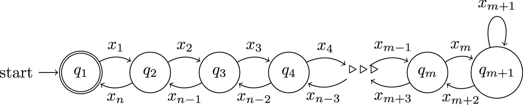
Fig.2
Deficiency tree for n = 4, see Remark 16.
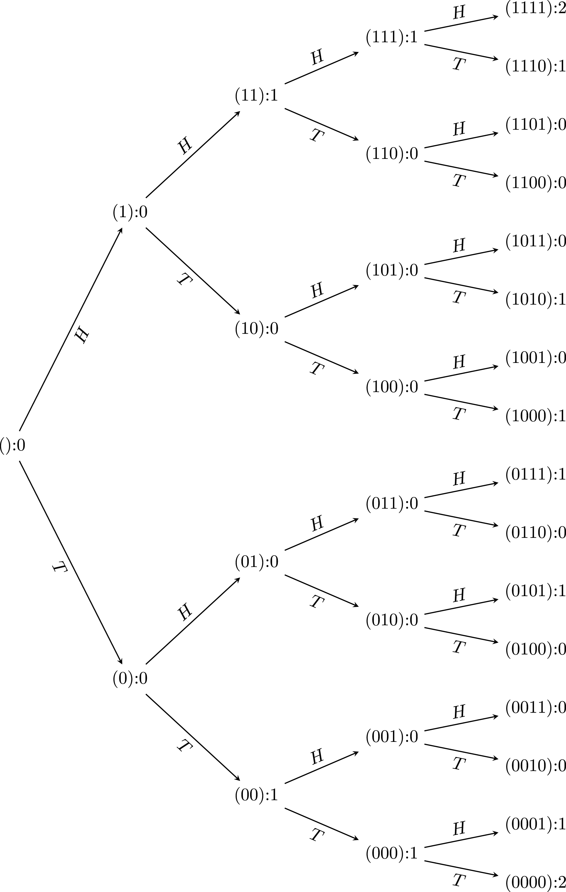
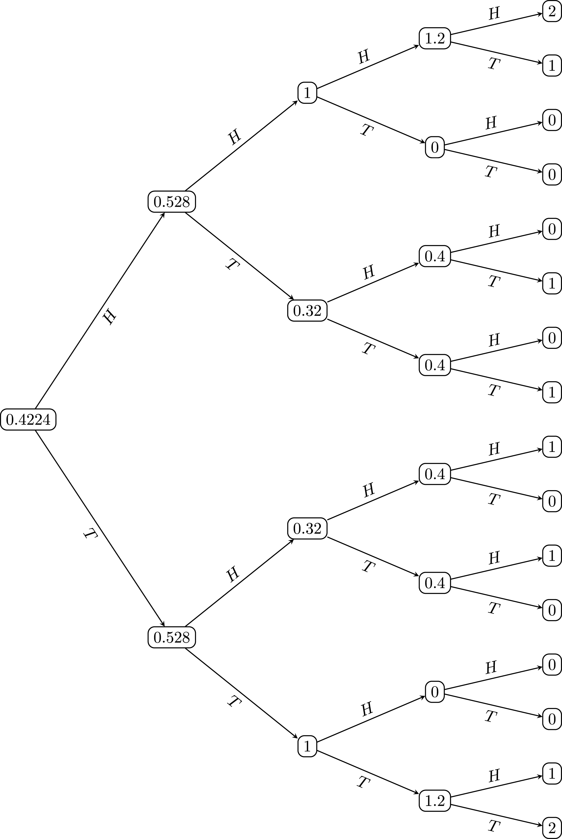
Table 1
Infinity and finiteness of option prices for various complexity deficiencies D
n
(x), for strings x of length n.
The conclusions labeled by ∴ (“therefore”) follow from the inequalities
| D n |
|
|
|
| n + c K - K (x) | ∴< ∞ | ∴< ∞ | <∞ (Theorem 9) |
| n + K (n) + c K - K (x) | <∞ (Theorem 10) | ∞ (Theorem 10) | ∴∞ |
| n + c C - C (x) | <∞ (Theorem 6) | ∞ (Theorem 7) | ∴∞ |
| n + c C - C (x ∣ n) | <∞ (Theorem 6) | ∞ (Theorem 7) | ∴∞ |
| ⌈n/2 ⌉ +1 - A N (x) | <∞? (Conjecture 15) | ∞? (Conjecture 15) | ∴∞? |
Table 2
Static versus dynamic exercise policies for nondeterministicautomatic complexity
| Length |
| ≤ | V n |
| 0 | 0 | = | 0 |
| 2 | 0.5 | = | 0.5 |
| 4 | 0.625 | < | 0.75 |
| 6 | 0.687 | < | 0.875 |
| 8 | 0.765 | < | 1.070 |
| 10 | 0.791 | < | 1.191 |
| 12 | 0.720 | < | 1.236 |
Table 3
Nondeterministic automatic complexity in the Hamming ball of radius 1 around 0 n , n = 23
| w | A N (w) |
| 023 | 1 |
| 0221 | 2 |
| 02110 | 3 |
| 020102 | 4 |
| 019103 | 5 |
| 018104 | 6 |
| 017105 | 7 |
| 016106 | 8 |
| 015107 | 9 |
| 014108 | 8 |
| 013109 | 8 |
| 0121010 | 8 |
| 0111011 | 7 |


